Sage Journals: Discover world-class research

Abstract

Electroencephalogram (EEG) data depict various emotional states and reflect brain activity. There has been increasing interest in EEG emotion recognition in brain–computer interface systems (BCIs). In the World Robot Contest (WRC), the BCI Controlled Robot Contest successfully staged an emotion recognition technology competition. Three types of emotions (happy, sad, and neutral) are modeled using EEG signals. In this study, 5 methods employed by different teams are compared. The results reveal that classical machine learning approaches and deep learning methods perform similarly in offline recognition, whereas deep learning methods perform better in online cross-subject decoding.

Keywords

electroencephalography emotion recognition online decoding cross-subject brain–computer interface

1 Introduction

Emotion is a vital part of humans and plays an important role in people’s daily communication [1]. Emotion recognition is the most fundamental and significant connection in emotion computing, as well as a critical research topic in the domains of brain–computer interface and human–computer interaction [2]. Traditional emotion recognition methods use auditory (speech) and visual (facial expression) attributes to predict human emotional responses, however, these external expressions cannot reliably detect emotion, especially when people subjectively hide their feelings [3]. At the moment, the acquisition of physiological reactions is gaining popularity in defining emotional states [4, 5]. Many research teams undertake emotion identification investigations using physiological signals such as breathing, body temperature, electromyography (EMG), electrocardiography (ECG), and electroencephalography (EEG). In comparison to other types of peripheral physiological signals, EEG is directly created by the human body’s central nervous system, which is intimately associated with the emotional state; hence, EEG can give deeper emotional information [6].

In recent years, emotion recognition based on scalp EEG has attracted considerable attention and has become a new direction of brain–computer interface (BCI), namely affective brain–computer interface (aBCI). EEG-based aBCI system mainly involves preprocessing, feature extraction, and classification, among which feature extraction of emotional EEG is a key factor affecting the effect of emotion recognition [7]. EEG signals have limited spatial resolution and frequency range, low signal-to-noise ratio, and are susceptible to the external environment and human activities such as respiration, ECG, and electrooculogram. How to get the most emotion-related EEG characteristics for emotional EEG is a fundamental scientific topic in the study of an aBCI system. EEG characteristics utilized for emotion identification are broadly classified into three types: time-domain characteristics, frequency-domain characteristics, and time-frequency characteristic. Time-domain features include Hjorth parameter [8], fractal dimension [9], higher-order crossing (HOC) [10], etc. Frequency domain features include differential entropy (DE) [11], differential asymmetry (DASM) [12], rational asymmetry (RASM) [13] and differential causality (DCAU) [14] in five classical frequency bands: delta (1–3 Hz), theta (4–7 Hz), alpha (8–13 Hz), beta (14–30 Hz) and gamma (31–50 Hz). Methods for extracting time-frequency features primarily include the short-time Fourier transform, wavelet transform, and others [15].

At the moment, the effective features utilized in EEG emotional recognition are mostly frequency domain features extracted from each EEG rhythm, and the DE feature has been demonstrated to be one of the most stable features with exceptional performance [16]. Meanwhile, several EEG emotion identification algorithms have been developed, with the majority of them being typical machine learning techniques. Consider the support vector machine (SVM) [17], k-nearest neighbor (KNN) [18], logistic regression (LR) [19] and random forest [20] supervised learning algorithms.

The existing EEG-based emotion recognition methods are mainly based on supervised machine learning. Wang et al. [21] compared power spectral density (PSD), wavelet, and nonlinear dynamic features with SVM. Zheng et al. [16] investigated the critical bands and channels using PSD, DE, and PSD asymmetric features, and obtained robust accuracy using a deep belief network. Significant variances in EEG signals exist between participants, limiting the generalization capabilities of the classifier learned in the single-subject classification context. This issue must yet be addressed.

BCI Controlled Robot Contest in World Robot Contest (WRC) held emotion recognition technology competition in 2021 [22]. The technological competition focused on the teams’ abilities to create and improve their algorithms, with an emphasis on the research team’s algorithms’ accuracy and reaction speed. The competition consists of a preliminary contest and a final contest. The preliminary contest was held in the cloud and the final contest was held on-site. The relevant competition data collected from the 2020 skill competition was used for the 2021 preliminaries. The 2021 finals will compete using real-time data gathered from the 2021 skill competition finals, ranking in real time based on the accuracy and efficiency of the calculation findings. Many university teams took part in the competition.

We compare the algorithms of several teams in this study. Some recommendations are made for future EEG-based emotion recognition across participants.

2 Background

2.1 Subjects and EEG recording

In the preliminary contest, 23 subjects (A1–A23) participated in the emotion recognition technology competition of WRC2021. Subjects wore the 62-channel EEG caps during the experiment while watching movie clips that might produce various emotional states, and EEG was recorded concurrently. Each experiment was recorded for about 1 h. The sampling rate of the raw EEG signals is 1000 Hz. The final contest had four individuals (F1–F4), and the EEG acquisition experimental parameters for the two phases were the same.

2.2 Emotion induction experiment

During an emotion induction experiment, subjects need to watch three categories of emotions (positive, neutral, and negative) videos. Each emotional video is a varied duration, and there is a time delay between clips for people to offer comments rest. To assure the induction impact of three types of emotions, the video clips utilized for emotion induction are rigorously analyzed and inspected (happy, sad, and neutral, the proportions are balanced). There are a total of 15 clips selected from Chinese films. There was a 5 s hint before each clip, 45 s for self-assessment. Subjects were asked to fill out a questionnaire immediately after seeing each video clip and express their emotional reactions to each video clip to collect feedback. The experimental process is shown in Fig. 1. Each subject participates in one experiment, and different subjects may watch different video clips. One video clip corresponds to one trial, one block comprises numerous trials (the number varies), and each subject’s data contains many blocks.

Fig. 1

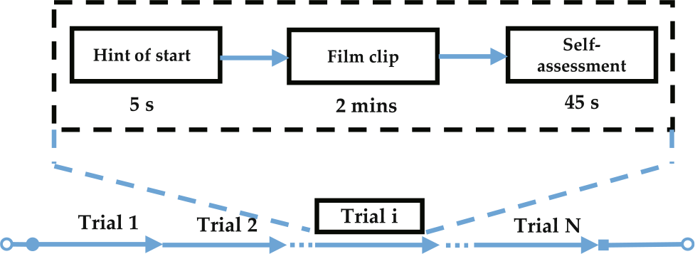
Time interval of one trial.

3 Methods

In this section, we describe the methods of preprocessing, feature extraction, and classification. The specific schemes used by different teams are detailed in Table 1. EEGNet-20, 8 [23] represents it has 20 temporal filters and 8 spatial filters. We utilized PSD as a feature and SVM with RBF kernel as a classifier as the baseline since it is simple and widely used in emotion identification tasks.

3.1 Preprocessing

Table 1 briefly presents the preprocessing setup of each method. Before our analysis, raw EEG data is passed through a 3rd- or 4th-order bandpass filter. Finally, EEG data is filtered between 0.5 and 49 or 50 Hz. The filtered continuous EEG data is segmented by extracting data segments while film clips are being shown. We downsampled the 62-channel EEG signals to 250 Hz to speed up the processing.

Table 1

Comparison of different methods.

Method	Preprocessing	Feature	Classifier
Baseline	Butter_bandpass: 0. 5Hz–50 Hz, order = 3	PSD	SVM (kernel = RBF)
M1	Butter_bandpass: 0.5 Hz–50 Hz, order = 3; MinMaxScaler: −200 : 200	PSD + log_PSD + DE	SVM (kernel = linear)
M2	Butter_bandpass: 0.5 Hz–50 Hz, order = 4	DE	Logistic regression
M3	Butter_bandpass: 0.5 Hz–49 Hz, order = 3; Butter_notch: 50 Hz, Q = 35	DE + Hjorth	Random Forest
M4	Butter_bandpass: 0.5 Hz–50 Hz, order = 3	–	EEGNet-20, 8

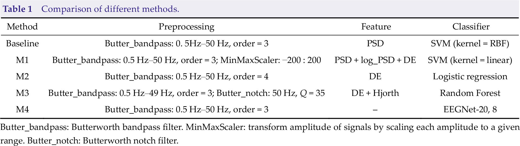
Butter_bandpass: Butterworth bandpass filter. MinMaxScaler: transform amplitude of signals by scaling each amplitude to a given range. Butter_notch: Butterworth notch filter.

3.2 Feature extraction

Three techniques have been used: PSD, DE, and Hjorth parameters.

3.2.1 Power spectral density

The power spectrum of the five aforementioned rhythms of EEG is a common feature. PSD may be computed under the premise that each state is ergodic by computing the Fourier transform of its temporal autocorrelation function. The PSD calculating procedure is as follows.

Let an EEG sample on an electrode be x(n). First, divide it into L segments, the i-th segment signal x_i (n) is shown in Eq. (1).

x_{i} (n) = x (n + i D)

where n = 0, 1,…, M; i = 0, 1,…, L −1. D is the translation length of the signal. Calculate the power spectral density psdi ( f ) of the i-th segment signal by periodic diagram method, as shown in Eq. (2).

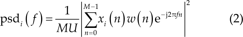
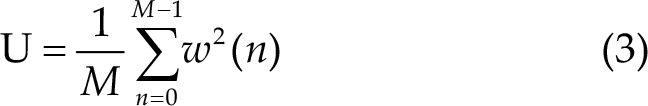
{psd}_{i} (f) = \frac{1}{M U} {| \sum_{n = 0}^{M - 1} x_{i} (n) w (n) e^{- j 2 π f n} |}^{2}

where, i = 0,1,…, L −1 , j is the imaginary unit. w(n) is the Hamming window function, which can reduce spectrum leakage, and its length is the same as that of each signal. U is the regularization coefficient of the window, which is used to reduce the influence of window function on power spectrum estimation. Its calculation method is shown in Eq. (3).

U = \frac{1}{M} \sum_{n = 0}^{M - 1} w^{2} (n)

Finally, the PSD estimated by the Welch method is the average value of each segment of PSD, as shown in Eq. (4).

psd (f) = \frac{1}{L} \sum_{i = 0}^{L - 1} {psd}_{i} (f)

3.2.2 Differential entropy

DE is a widely used feature in EEG-based emotion recognition, and can be defined as follow:

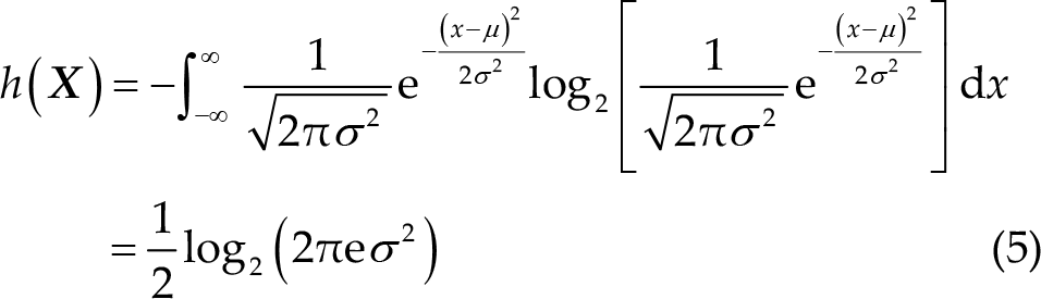
\begin{array}{l} h (X) = - \int_{- \infty}^{\infty} \frac{1}{\sqrt{2 π σ^{2}}} e^{- \frac{{(x - μ)}^{2}}{2 σ^{2}}} \log_{2} [\frac{1}{\sqrt{2 π σ^{2}}} e^{- \frac{{(x - μ)}^{2}}{2 σ^{2}}}] d x \\ = \frac{1}{2} \log_{2} (2 π e σ^{2}) \end{array}

where the time series X obeys Gaussian distribution N(μ,σ ² ). DE is used to construct features in five rhythms of EEG.

3.2.3 Hjorth parameters

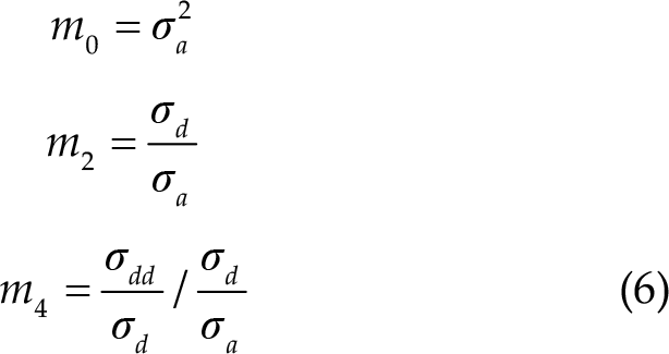
There are three statistical properties introduced by Bo Hjorth [8]. The Hjorth parameters, which assess the signal’s complexity, are as follows [24]:

Activity parameter (m ₀) represents the power of the signal.

Mobility parameter (m ₂) is the ratio of the standard deviation of the first derivative of the signal to the standard deviation of the original signal.

Complexity parameter (m ₄) represents the change of frequency.

The discrete formula used to calculate these parameters is based on the following derivation (Eq. (6)):

\begin{matrix} m_{0} = σ_{a}^{2} \\ m_{2} = \frac{σ_{d}}{σ_{a}} \\ m_{4} = \frac{σ_{d d}}{σ_{d}} / \frac{σ_{d}}{σ_{a}} \end{matrix}

where $σ_{d}^{2}$ is the variance of the EEG signal a. σd is the standard deviation of the first derivative of a. σ_dd is the standard deviation of the second derivative of a.

3.3 Feature smoothing

The majority of existing EEG-based emotion detection techniques translate EEG signals to static discrete emotional states, which may be illogical given that emotion is not a discrete psychophysiological state [25, 26]. It is necessary to smooth the features we extracted above because emotion usually varies smoothly while the features contained many rapid fluctuations.

In this research, we employed the traditional moving average (MA) approach to remove components that are not related to emotional states. Specifically, we applied MA with a window of 10 s to smooth features. We did not apply MA to M5 because it accepts raw EEG data as input. To accelerate the convergence of the model training, we further normalized the smoothed features.

4 Results & discussion

In this section, we briefly present the experimental setup and results.

For offline analysis in the preliminary contest, to evaluate the performance of each algorithm a cross-validation (CV) and a hold-out (HO) analysis were conducted. The CV analysis was conducted in a 10-fold setting, where 9 folds are used for training and the remaining 1 fold for testing. For cross-subject classification, a HO analysis is utilized. The whole data for a specific subject is utilized for testing in the HO analysis, and model training is conducted on the data for all other subjects. While in online analysis in the final contest, every team must give real-time feedback when the fire-new and consecutive emotional EEG signals were obtained. Notably, no team has access to all individuals’ EEG signals, which implies that players may only train models using data from other participants. In this scenario, the competition organizer provided a training dataset. This dataset includes four healthy volunteers (F1–F4), and the 62-channel EEG signals were originally captured at 1000 Hz, following the final contest arrangement. In this research, we train models for online analysis in the final contest utilizing this four-subjects dataset.

Table 2 presents the 10-fold CV accuracies for all subjects in the preliminary contest. M2, which only extracts DE features matched the performance of the best performing method for most subjects resulting in the best average classification accuracy. It’s worth noting that M1 and M3, which combine DE characteristics and other feature sets, perform poorly. This phenomenon is caused by serially concatenating two or more feature sets into a composite feature set. Vectors often have very large dimensions, which can place a significant strain on the emotion classification job and lead to overfitting issues [27]. In this instance, using appropriate feature fusion algorithms may be an ideal solution for minimizing side effects.

Table 2

Classification accuracy (%) of different algorithms in offline EEG emotion recognition of a single subject in the preliminary contest.

Subject	Method
Subject	Baseline	M1	M2	M3	M4
A1	85.89/96.64	73.45/96.38	82.50/97.47	77.92/93.72	72.71
A2	81.00/95.93	77.58/95.46	86.21/96.91	79.37/93.64	85.07
A3	88.69/96.67	81.35/97.50	87.57/97.76	80.70/95.35	88.37
A4	75.04/95.34	70.30/94.52	80.02/95.38	64.35/93.18	75.57
A5	93.22/96.02	81.47/98.67	92.19/99.17	77.32/97.48	92.81
A6	91.99/96.52	82.79/97.44	91.46/99.06	83.49/89.97	92.32
A7	91.75/96.64	86.74/98.91	92.75/99.41	87.13/97.82	90.00
A8	92.10/96.52	85.47/98.38	92.90/99.38	85.88/98.96	87.19
A9	87.74/96.76	81.50/96.70	87.63/98.14	81.53/95.88	94.04
A10	84.89/96.58	74.54/96.32	85.89/97.67	77.93/94.80	81.82
A11	84.09/95.67	82.97/95.29	90.75/98.08	85.54/96.31	90.89
A12	90.69/95.46	84.71/98.17	91.51/98.88	78.79/96.01	90.49
A13	87.89/95.93	84.80/98.00	91.57/98.91	85.69/92.32	92.96
A14	82.06/96.79	75.46/95.93	82.23/95.26	74.17/99.86	82.61
A15	97.85/96.64	95.79/100.00	97.97/99.91	91.78/93.74	92.56
A16	70.56/95.16	65.31/90.77	72.14/90.39	65.95/92.70	68.72
A17	68.04/98.13	57.09/91.31	71.69/91.16	50.56/93.87	38.03
A18	69.29/95.85	64.78/90.27	70.98/90.83	58.67/88.19	64.44
A19	71.63/97.63	61.78/93.71	73.74/94.33	70.40/92.39	65.78
A20	74.21/96.20	62.73/93.80	71.19/92.43	64.46/96.83	61.09
A21	76.85/95.50	67.98/95.13	74.51/93.53	65.30/96.83	77.31
A22	78.81/95.79	62.55/94.30	73.92/93.41	59.18/94.62	59.53
A23	83.65/94.87	73.18/94.27	83.80/96.02	74.79/98.92	70.66
Mean	82.95/96.23	75.36/95.71	83.70/96.24	74.82/94.93	78.91
Std	8.37/0.75	9.69/2.56	8.36/2.96	10.45/2.80	14.10

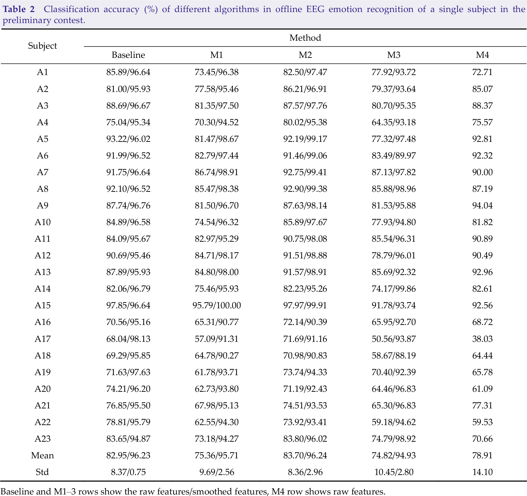
Baseline and M1–3 rows show the raw features/smoothed features, M4 row shows raw features.

The result of the HO analysis can be seen in Table 3. It is not straightforward to see that each approach has a considerable decline in performance (up to 27.8% inaccuracy), which is due to the low generalizability of the EEG characteristics in representing emotional information across people [28]. We see that all methods have a slight difference in performance ranking. M2 and baseline perform the best, whereas M1 and M3 perform the poorest. M4, the sole deep learning approach, performs poorly in both CV analysis and HO analysis.

Table 3

Classification accuracy (%) of different methods in offline EEG emotion recognition across subjects in the preliminary contest.

Subject	Method
	Baseline	M1	M2	M3	M4
A1	57.78/57.54	56.42/62.17	60.28/64.70	56.24/60.36	38.92
A2	57.51/61.67	53.48/60.02	52.98/62.32	60.06/61.32	54.38
A3	61.52/64.17	57.72/61.20	61.28/60.52	64.23/65.94	65.67
A4	47.94/48.56	48.64/51.97	46.02/47.55	45.42/50.24	44.29
A5	55.92/54.89	53.62/50.03	59.69/65.65	49.88/55.81	49.51
A6	61.26/62.61	58.13/61.14	61.99/65.26	51.88/63.05	59.41
A7	58.96/58.34	52.21/64.47	61.55/65.09	44.44/58.61	55.91
A8	67.32/73.04	62.14/68.47	67.62/67.71	64.48/69.02	59.06
A9	65.76/73.92	60.14/71.51	67.15/69.03	57.66/67.43	58.08
A10	59.34/59.07	51.44/56.75	61.58/61.84	49.64/57.31	39.01
A11	58.22/57.19	57.51/57.51	58.81/55.19	61.74/58.92	68.42
A12	57.33/50.47	47.61/57.84	60.70/64.91	47.44/57.16	60.10
A13	63.88/61.90	62.99/63.11	64.44/65.76	61.15/65.28	60.79
A14	57.37/59.58	57.16/62.46	59.16/56.01	55.23/59.85	62.12
A15	65.44/63.88	61.14/59.99	63.55/62.82	59.96/62.53	64.58
A16	50.33/49.76	49.64/50.62	48.55/51.28	42.22/48.47	41.36
A17	42.26/43.71	39.82/43.53	39.08/42.49	45.58/42.36	35.35
A18	45.01/49.05	43.71/47.72	43.71/44.78	45.60/45.11	49.30
A19	45.49/47.36	41.63/51.19	43.95/41.69	45.57/48.76	44.09
A20	52.76/54.18	45.88/51.69	52.37/53.65	54.98/55.16	39.87
A21	43.26/55.49	41.60/45.91	41.13/45.85	44.18/49.19	44.34
A22	48.93/50.98	47.06/47.83	49.97/50.74	45.93/50.23	55.56
A23	61.36/66.44	52.43/59.64	60.03/55.43	58.05/57.70	62.96
Mean	55.87/57.56	52.27/56.82	55.90/57.69	52.68/56.94	52.74
Std	7.33/7.70	6.77/7.23	8.39/8.49	7.09/7.12	9.81

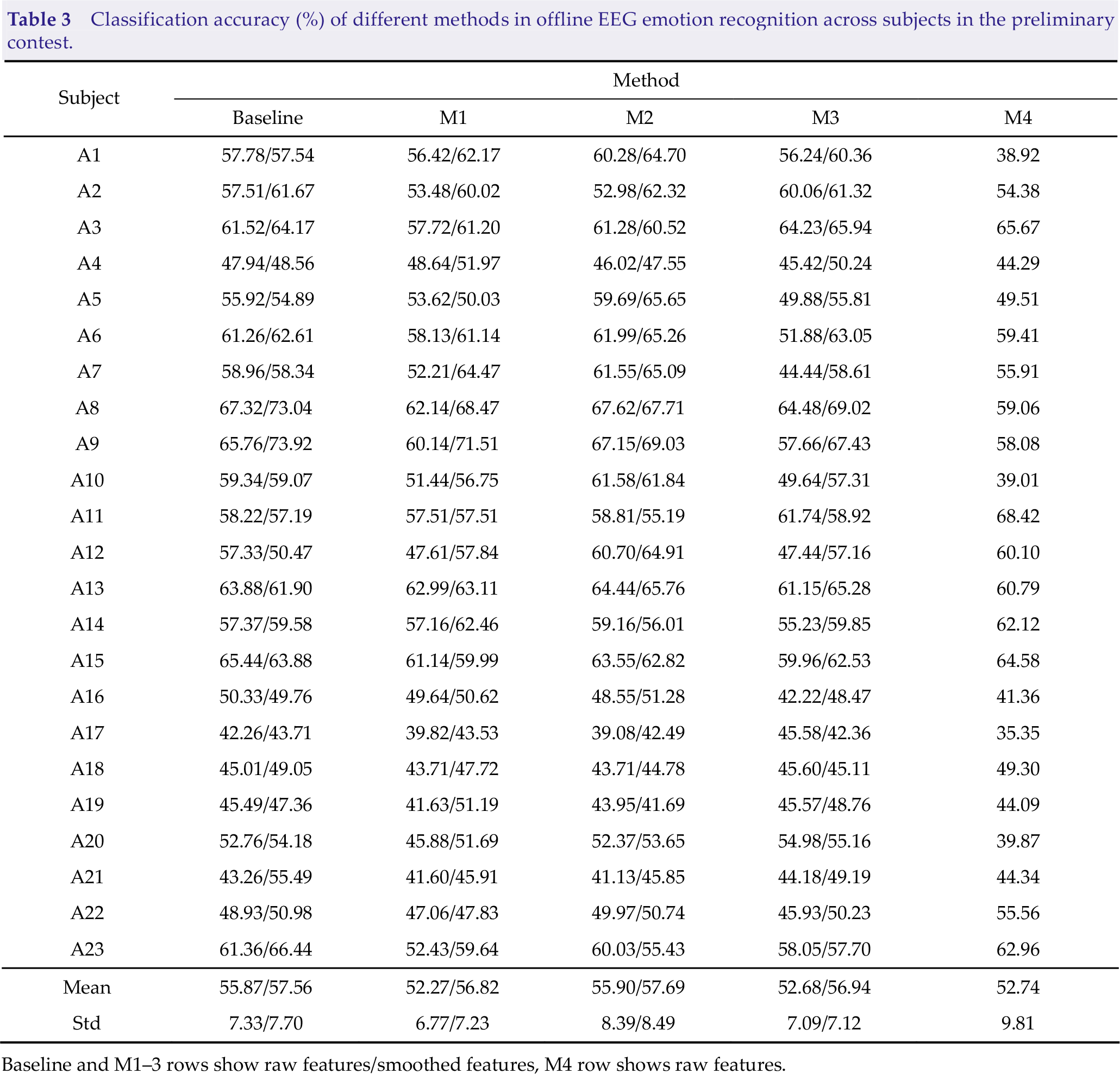
Baseline and M1–3 rows show raw features/smoothed features, M4 row shows raw features.

Table 4 depicts the cross-subject classification accuracy in the final contest (online analysis). It can be shown that the single deep learning technique (M4) outperforms M3, which differs from the findings of the offline study. In contrast to offline analysis, subjects are not in a sufficiently quiet environment during the online emotion recognition task, which led to the collected EEG signal would contain obvious environmental noises. As a result, we suspect that the reason M4 outperforms M3 is that M4 extracted relatively robust features from these noisy signals, which can overcome the interference of noises generated by the complex environment of the playing field and benefits from deep learning techniques’ strong learning ability. Similarly, each technique performs worse under online analysis, probably for two reasons: a) complicated ambient sounds made extracting important characteristics more difficult; and b) participants were distracted by their surroundings, making it impossible to elicit strong emotions.

Table 4

Classification accuracy(%) of different methods in online EEG emotion recognition across subjects in the final contest. Each session has three blocks.

Subject	Block	Method
		Baseline	M1	M2	M3	M4
F1	1	44.27/44.35	33.36/34.20	50.98/51.65	32.10/36.40	19.74
	2	49.39/49.12	40.12/42.55	32.67/33.53	38.12/39.15	39.87
	3	35.43/37.21	52.46/54.11	45.33/46.71	37.06/36.24	45.13
F2	1	40.76/41.25	38.60/37.14	39.62/42.11	39.33/40.15	37.88
	2	37.04/38.54	36.94/33.39	45.17/45.55	41.65/42.80	38.33
	3	45.80/46.91	30.45/31.22	44.84/43.13	40.67/41.69	41.97
F3	1	43.22/44.12	29.30/30.15	39.51/42.24	34.18/36.53	60.17
	2	37.07/36.51	39.60/41.97	35.27/38.03	42.27/43.71	55.26
	3	46.49/44.25	35.75/37.54	38.25/39.01	36.79/38.66	39.08
F4	1	41.03/42.38	49.01/51.29	58.11/58.37	36.54/36.19	57.68
	2	33.45/35.11	43.65/47.31	28.28/31.63	37.89/39.62	52.17
	3	35.91/35.42	42.65/45.19	29.49/32.78	40.76/40.99	52.29
Mean		40.82/41.26	39.32/40.51	41.46/42.06	38.11/39.34	45.05
Std		4.86/4.47	11.68/7.53	7.40/7.56	2.90/2.53	10.82

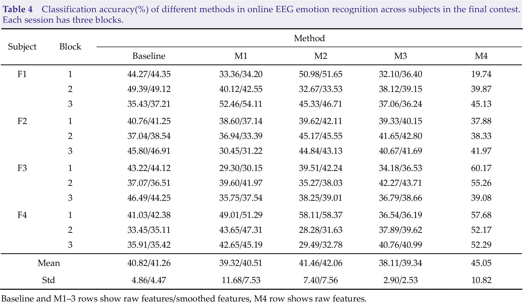
Baseline and M1–3 rows show raw features/smoothed features, M4 row shows raw features.

We also evaluate the performance of the feature smoothing algorithms. Fig. 2 presents an example of features before and after smoothing. The original features fluctuate greatly, while the smoothed features change slowly. From Tables 2–4, we find that the classification accuracy of smoothed features is better than that of original features. Especially in CV analysis in offline emotion recognition, the means of the classification accuracies of M1 in percentages achieves up to 20.35% higher after applying MA. Another intriguing occurrence is that MA has a lower capacity to enhance accuracy in HO analysis in offline emotion identification, with a maximum improvement of 4.55%, and much lower in online emotion detection, with a maximum improvement of 1.23%. This result can be attributed to the huge individual difference in EEG signals, which makes it complex to extract features with strong generalization ability and limits the upper limit of classification performance of algorithms. To summarize, feature smoothing is an essential procedure for improving classification performance.

Fig. 2

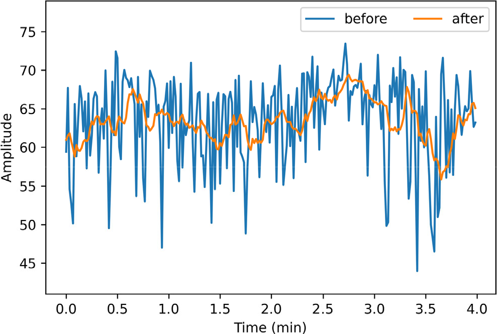
Difference between features before and after smoothing.

The time spent by the algorithm is an important metric in online emotion recognition tasks. The time required by each method for feature extraction and classification of a single sample (1-second EEG signal with 62 channels) is illustrated in Fig. 3. The baseline approach takes the shortest time, only 1.53 ms, while the rest of the methods take about the same time. M4, being a deep learning algorithm, takes the second-longest time, which is understandable given the complexity of deep learning models. M1 takes longer than M4, which might be because M1 extracts more characteristics.

Fig. 3

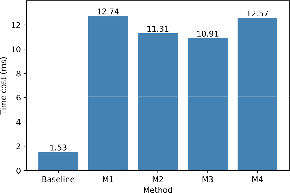
Time cost of each method in online emotion recognition.

5 Conclusion

This work systematically studies the offline and online performance of the top 5 methods in the emotion recognition technology competition of WRC2021 on the emotion recognition task. We experimentally established that EEGNet-20,8 is more suited for online emotion categorization, despite its poor performance in offline analysis. We also discover that there is no substantial performance benefit from just serially concatenating the DE feature set with other feature sets into a combined feature vector, implying that using a suitable feature process technique is critical. One possible way of dealing with this issue is to adopt suitable feature fusion techniques [29 –31], which could be studied in the future.

It is worth noting that EEG signals are a kind of unsteady signals and have individual differences. In general, it is challenging to build accurate cross-subject emotion identification models using traditional machine learning methods. Transfer learning offers a possible solution to the problem of individual differences in emotion recognition models [32 –34]. It is a great choice that uses transfer learning to improve higher classification accuracy in future online emotion identification tasks.

Most of the existing emotion-inducing experiments are in the laboratory environment, and the subjects induce specific emotions by watching stimulating pictures or videos. The preceding section’s results reveal that online decoding accuracy is much lower than offline decoding accuracy, which might be attributed to inadequate stimulus induction in the real scene. This discovery raises an essential question: how to rapidly collect high-quality emotional EEG data in real-world complicated scenes™ Solving this problem might be an interesting and challenging research subject.

Footnotes

Conflict of interests

All contributing authors have no conflict of interests.

Funding

This work was supported in part by the National Natural Science Foundation of China (Grant Nos. U21A20485, 61976175).

Authors’ contribution

Chao Tang: Methodology, writing-original draft. Yunhuan Li: Software, formal analysis. Badong Chen: Reviewing, editing, and supervision.

References

Poria

Cambria

Bajpai

etal. A review of affective computing: from unimodal analysis to multimodal fusion. Inf Fusion 2017, 37: 98–125.

Song

Zheng

Song

etal. EEG emotion recognition using dynamical graph convolutional neural networks. IEEE Trans Affect Comput 2020, 11(3): 532–541.

Nie

Wang

Shi

etal. EEG-based emotion recognition during watching movies. In 2011 5th International IEEE/EMBS Conference on Neural Engineering, Cancun, Mexico, 2011, pp 667–670.

Appriou

Cichocki

Lotte

. Modern machine-learning algorithms: for classifying cognitive and affective states from electroencephalography signals. IEEE Syst Man Cybern Mag 2020, 6(3): 29–38.

Torres-Valencia

Álvarez-López

Orozco-Gutiérrez

. SVM-based feature selection methods for emotion recognition from multimodal data. J Multimodal User Interfaces 2017, 11(1): 9–23.

Liu

etal. Emotion recognition from multichannel EEG signals using K-nearest neighbor classification. Technol Health Care 2018, 26(S1): 509–519.

Yin

Liu

Chen

etal. Locally robust EEG feature selection for individual-independent emotion recognition. Expert Syst Appl 2020, 162: 113768.

Hjorth

. EEG analysis based on time domain properties. Electroencephalogr Clin Neurophysiol 1970, 29(3): 306–310.

Ansari-Asl

Chanel

Pun

T. A

channel selection method for EEG classification in emotion assessment based on synchronization likelihood. In 2007 15th European Signal Processing Conference, Poznan, Poland, 2007, pp 1241–1245.

10.

Petrantonakis

Hadjileontiadis

. Emotion recognition from EEG using higher order crossings. IEEE Trans Inf Technol Biomed 2010, 14(2): 186–197.

11.

Duan

Zhu

. Differential entropy feature for EEG-based emotion classification. In 2013 6th International IEEE/EMBS Conference on Neural Engineering (NER), San Diego, CA, USA, 2013, pp 81–84.

12.

Bos

D O.

EEG-based emotion recognition: The influence of visual and auditory stimuli. https://www.semanticscholar.org/paper/EEG-based-Emotion-Recognition-The-Influence-of-and-Bos/5097b37a30b8d7a8d2bb03b307be5bf5deab73c4 (accessed Jun 6, 2022).

13.

Lin

Wang

Jung

etal. EEG-based emotion recognition in music listening. IEEE Trans Biomed Eng 2010, 57(7): 1798–1806.

14.

Lin

Hsu

Jung

Exploring day-to-day variability in the relations between emotion and EEG signals. In Foundations of Augmented Cognition. AC 2015. Lecture Notes in Computer Science. Vol 9183. Schmorrow DD, Fidopiastis CM, Eds. Cham: Springer, 2015, pp 461–469.

15.

Mohammadi

Frounchi

Amiri

. Wavelet-based emotion recognition system using EEG signal. Neural Comput Appl 2017, 28(8): 1985–1990.

16.

Zheng

. Investigating critical frequency bands and channels for EEG-based emotion recognition with deep neural networks. IEEE Trans Auton Ment Dev 2015, 7(3): 162–175.

17.

Noble

. What is a support vector machine™ Nat Biotechnol 2006, 24(12): 1565–1567.

18.

Mehmood

Lee

. Emotion classification of EEG brain signal using SVM and KNN. In 2015 IEEE International Conference on Multimedia & Expo Workshops, Turin, Italy, 2015, pp 1–5.

19.

Pan

Shi

etal. EEG-based emotion recognition using logistic regression with Gaussian kernel and Laplacian prior and investigation of critical frequency bands. Appl Sci 2020, 10(5): 1619.

20.

Veeramallu

GKP

Anupalli

Jilumudi

etal. EEG based automatic emotion recognition using EMD and random forest classifier. In 2019 10th International Conference on Computing, Communication and Networking Technologies (ICCCNT), Kanpur, India, 2019, pp 1–6.

21.

Wang

Nie

. Emotional state classification from EEG data using machine learning approach. Neurocomputing 2014, 129: 94–106.

22.

World Robot Contest. http://www.worldrobotconference.com/cn/about/134.html, (accessed Jun 6, 2022)

23.

Lawhern

Solon

Waytowich

etal. EEGNet: a compact convolutional neural network for EEG-based brain-computer interfaces. J Neural Eng 2018, 15(5): 056013.

24.

Vourkas

Micheloyannis

Papadourakis

. Use of ANN and Hjorth parameters in mental-task discrimination. In 2000 First International Conference Advances in Medical Signal and Information Processing, Bristol, UK，2000, pp 327–332.

25.

Zheng

Zhu

. Identifying stable patterns over time for emotion recognition from EEG. IEEE Trans Affect Comput 2019, 10(3): 417–429.

26.

Fontaine

JRJ

Scherer

Roesch

etal. The world of emotions is not two-dimensional. Psychol Sci 2007, 18(12): 1050–1057.

27.

Mao

. Feature regrouping for CCA - based feature fusion and extraction through normalized cut. In 2018 21st International Conference on Information Fusion (FUSION), Cambridge, UK, 2018, pp 2275–2282.

28.

Song

Zhang

etal. Exploring EEG features in cross-subject emotion recognition. Front Neurosci 2018, 12: 162.

29.

Cao

Guo

etal. Multiple feature fusion by subspace learning. In CIVR ‘08: Proceedings of the 2008 International Conference on Content-based Image and Video Retrieval, New York, USA, 2008, pp 127–134.

30.

Feng

etal. Multiple feature fusion via weighted entropy for visual tracking. In 2015 IEEE International Conference on Computer Vision, Santiago, Chile, 2015, pp 3128–3136.

31.

Hou

Sun

Xia

. Feature fusion using multiple component analysis. Neural Process Lett 2011, 34(3): 259–275.

32.

Lin

Jung

. Improving EEG-based emotion classification using conditional transfer learning. Front Hum Neurosci 2017, 11: 334.

33.

Zheng

W L

B L.

Personalizing EEG-based affective models with transfer learning. In Proceedings of the Twenty-Fifth International Joint Conference on Artificial Intelligence, New York, USA, 2016, pp 2732–2738.

34.

Wan

Yang

Huang

etal. A review on transfer learning in EEG signal analysis. Neurocomputing 2021, 421: 1–14.

Comparison of cross-subject EEG emotion recognition algorithms in the BCI Controlled Robot Contest in World Robot Contest 2021

Abstract

Keywords

1 Introduction

2 Background

2.1 Subjects and EEG recording

2.2 Emotion induction experiment

3 Methods

3.1 Preprocessing

3.2 Feature extraction

3.2.1 Power spectral density

3.2.2 Differential entropy

3.2.3 Hjorth parameters

3.3 Feature smoothing

4 Results & discussion

5 Conclusion

Footnotes

Conflict of interests

Funding

Authors’ contribution

References