Sage Journals: Discover world-class research

Abstract

Electroencephalography (EEG) is a powerful tool for investigating the brain bases of human psychological processes non‐invasively. Some important mental functions could be encoded by resting‐state EEG activity; that is, the intrinsic neural activity not elicited by a specific task or stimulus. The extraction of informative features from resting‐state EEG requires complex signal processing techniques. This review aims to demystify the widely used resting‐state EEG signal processing techniques. To this end, we first offer a preprocessing pipeline and discuss how to apply it to resting‐state EEG preprocessing. We then examine in detail spectral, connectivity, and microstate analysis, covering the oft‐used EEG measures, practical issues involved, and data visualization. Finally, we briefly touch upon advanced techniques like nonlinear neural dynamics, complex networks, and machine learning.

Keywords

resting‐state EEG preprocessing spectral analysis connectivity analysis microstate analysis

1 Introduction

Psychologists devote their efforts to understanding the mental processes of individuals [1]. One of the most important lines in psychological research is to unravel how these processes are implemented in the brain. Theoretical and ethical considerations call for noninvasive techniques to study the brain bases of human psychological processes. Electroencephalography (EEG) is among the most popular methods to image the brain at work noninvasively, thanks to its outstanding temporal resolution and relatively low costs.

Simply put, electroencephalography is the technique of recording the electrical activity of the brain at the scalp. Etymologically speaking, “electro‐” means “electricity”, “encephalo‐” means “of the brain”, and “‐graphy” means “to write”. The record or tracing of such activity is termed electroencephalogram, which is (somewhat confusingly) also abbreviated as EEG. The electrical activity of the brain was first detected by British physician Richard Caton more than 140 years ago [2]. German psychiatrist Hans Berger then showed that this kind of activity could be measured at the scalp without opening the skull [3]. However, neurophysiologists at that time thought that the slow brain waves Berger observed were likely to be artifacts [4] until the phenomenon was confirmed by Edgar Adrian and Matthews [5], Jasper and Carmichael [6], and Gibbs, Davis, and Lennox [7]. From then on, EEG has been accepted by the scientific community and gained popularity gradually [4].

From a neurophysiological perspective, EEG reflects the postsynaptic potentials (PSPs), resulting from the binding of neurotransmitters to the receptors in the postsynaptic membrane [4, 8, 9]. These PSPs generate electric fields surrounding the neurons. However, the electric field from a single neuron is too weak to be observed from outside the head. It has been estimated that 10,000 to 50,000 neurons must be synchronously activated for their signals to be detected using scalp EEG [10]. Yet, a large number of active neurons are only a necessary condition for EEG recording; these neurons also have to be active in the “right” way. Specifically, the orientations of neurons should be similar; otherwise, the electric fields generated will cancel each other out. Fortunately, the pyramidal neurons in the cerebral cortex meet this requirement. These cells are perpendicular to the cortical surface. The corresponding electric fields sum together and pass through the brain tissue, the skull, and the scalp to be finally detected by scalp EEG electrodes. As a result, the activity of pyramidal neurons accounts for the majority of EEG recorded at the scalp, while other neurons contribute very little to the generation of EEG [4].

The neural origins of EEG have three major implications. First, EEG provides a direct measure of the electrical activity of neurons; this feature contrasts starkly with the blood‐oxygen-level‐dependent (BOLD) signal captured by functional magnetic resonance imaging (fMRI), which only measures the neuronal activity indirectly by the corresponding hemodynamic and metabolic changes [11]. Second, the temporal resolution of EEG is extremely high (typically at the level of milliseconds), which stands out from other noninvasive neural imaging techniques. Third, the spatial resolution of EEG is poor, since the signal recorded from one electrode is the mixture of PSPs from all possible brain regions, not just the one under that electrode [8, 9].

These features partly explain why EEG is popular, especially when high spatial resolution is not indispensable for a study. Indeed, EEG has been widely adopted in virtually all topics of psychological research: pain [12, 13], vision [14], movement [15], attention [16], memory [17], decision‐making [18], language processing [19], emotion [20], social cognition [21], moral evaluation [22], to name but a few.

The usefulness and popularity of EEG notwithstanding, psychologists who attempt to make full use of EEG to investigate the neural bases of mental processes face a hurdle. Extracting all psychologically meaningful features EEG can provide requires complicated signal processing techniques, with which many psychologists might be unfamiliar. We thus, through two articles, try to offer a short but practical introduction to EEG signal processing with MATLAB scripts available in the supplementary material, in the hope of facilitating the applications of EEG techniques by psychologists.

EEG can be categorized into two groups according to the endogeneity of recorded activity. One group is resting‐state EEG, which refers to endogenous or intrinsic neural activity without a specific stimulus or task imposed; the other is task‐related EEG, which is induced or evoked by an exogenously imposed stimulus or task [23]. As the first one of our introductions to EEG processing, this article focuses on resting‐state EEG analysis. Traditionally, resting‐state EEG is recorded for basic and clinical studies in the eyes‐closed and/or eyes‐open condition for a few minutes [24]. Although participants simply “rest” and are asked to do nothing, resting‐state EEG could provide plenty of important information. For example, some features of spontaneous alpha band oscillations could reflect individual differences in cognitive ability [25].

In the rest of this review, we first describe steps of preprocessing to denoise EEG data. We then discuss how to perform spectral, connectivity, and microstate analysis on resting‐state EEG data. Further, we briefly touch upon some advanced data analysis techniques, such as nonlinear dynamics, complex network, and machine learning. Finally, we conclude with a short summary of measures obtainable from resting‐state EEG data analysis.

2 EEG Preprocessing

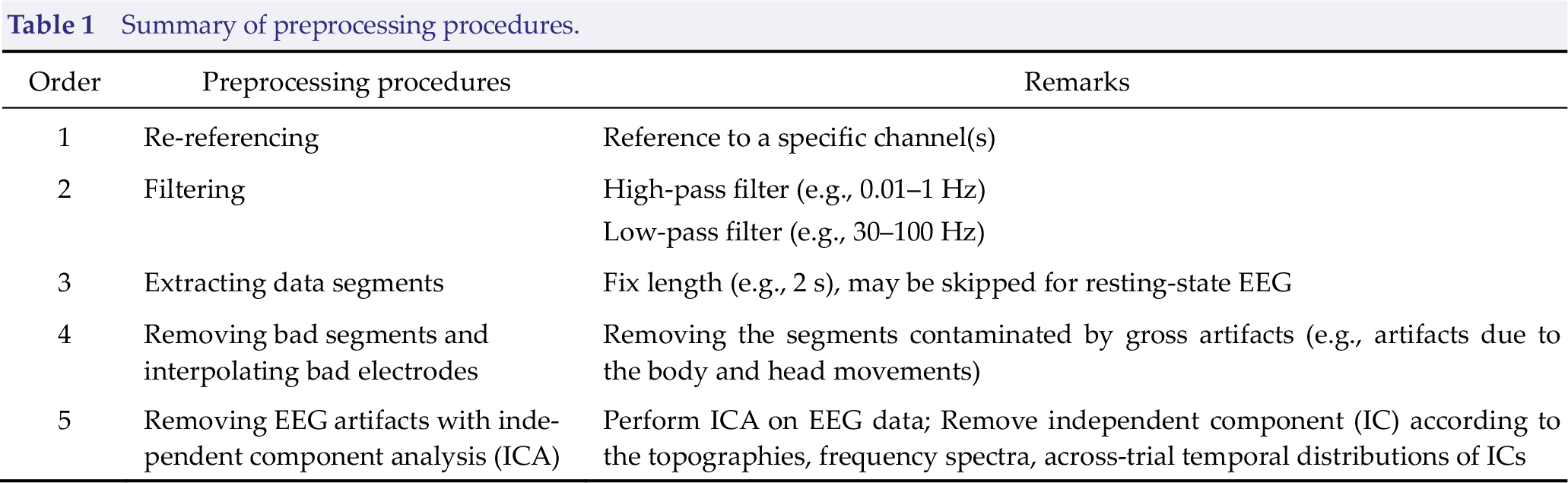
Raw EEG data are a mixture of neuronal activity, physiological artifacts, and non‐physiological noise. Therefore, it is essential to perform a preprocessing procedure to clean noise, remove artifacts, and ultimately improve the signal‐to-noise ratio (SNR) of the EEG data. The preprocessing procedure for resting‐state EEG comprises re‐referencing, filtering, extracting data segments, removing bad segments, and interpolating bad electrodes, as well as removing additional EEG artifacts with independent component analysis (ICA) (Table 1) [26]. The entire procedure can be performed in the open source MATLAB toolbox EEGLAB (Fig. 1) [27]. Note that the order of the steps in Table 1 is by no means fixed or applicable to all occasions. The study design, the nature of data, and the analysis techniques may impact the preprocessing procedure [26]. For example, re‐referencing should be conducted after bad electrode interpolation if the average reference is adopted; data segments may be extracted after ICA in some cases. As a result, the pipeline should be regarded as a convenient guide and could be modified accordingly in practice.

Table 1.

Summary of preprocessing procedures.

Order	Preprocessing procedures	Remarks
1	Re‐referencing	Reference to a specific channel(s)
2	Filtering	High‐pass filter (e.g., 0.01–1 Hz) Low‐pass filter (e.g., 30–100 Hz)
3	Extracting data segments	Fix length (e.g., 2 s), may be skipped for resting‐state EEG
4	Removing bad segments and interpolating bad electrodes	Removing the segments contaminated by gross artifacts (e.g., artifacts due to the body and head movements)
5	Removing EEG artifacts with independent component analysis (ICA)	Perform ICA on EEG data; Remove independent component (IC) according to the topographies, frequency spectra, across‐trial temporal distributions of ICs

Fig. 1.

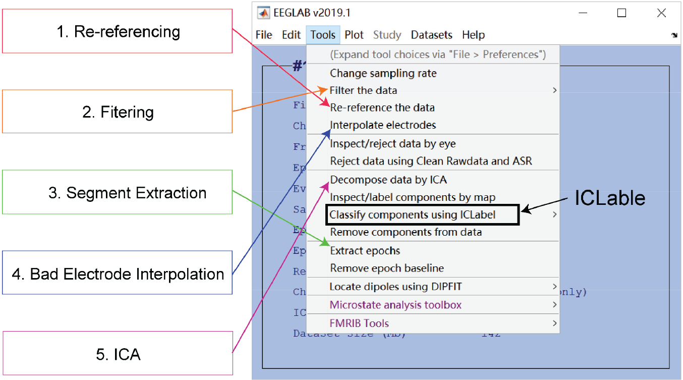
Preprocessing in EEGLAB. Five major steps for prepossessing resting‐state EEG data are re‐referencing, filtering, segment extraction, bad electrode interpolation, and artifacts removal using independent component analysis (ICA). EEGLAB tools for doing them are indicated by colored arrows. ICLable provides automatic independent component classification after ICA has been performed.

2.1 Re‐referencing

EEG records electrical potentials, which are, by definition, the potential differences between two sites: the active electrode and the ground electrode. However, the ground electrode contains electrical noise since it is connected to the EEG machine. To eliminate such noise, we choose a third electrode called the “reference” and the electrical signal recorded from electrode X equals (electrode X – ground) – (reference – ground) [4]. As a result, the signal is the potential difference between electrode X and the reference.

The byproduct is that any activity in the reference electrode is reflected in the signals sampled from all active electrodes [8]. Thus, we should make sure that the reference electrode is properly placed and its signal is good and clean [28]. Aside from these requirements, the choice of reference electrode during EEG recording does not matter much. What truly matters is the choice of the re‐reference electrode, to which we re‐reference the raw data offline [29]. Recall that the signal in electrode X is the voltage of electrode X minus that of the reference electrode. Re‐referencing does the same thing, except that it is performed after the raw signals have been collected. The simple subtraction operation also guarantees that re‐referencing would not distort the data. To avoid potential confusion, we can call the re‐reference electrode as “the new reference electrode”, or simply “the reference”. Note that the reference need not be a single electrode, but can be the average of several electrodes. Indeed, the average of all electrodes (namely the average reference) is popularly adopted in practice.

Given that it affects signals of all electrodes, the reference is required to be set at a remote position and has a stable (or ideally zero) potential. However, a perfect reference electrode simply does not exist [4, 30]. We, therefore, must make tradeoffs on which reference to use. The choice of reference depends on a variety of factors, including the position of the chosen electrode, the total number of electrodes, the brain regions of interest, and the analysis to be performed [31, 32]. Some guiding principles are: (1) choose a reference far away from the electrodes of interest; (2) do not reference to a site biased toward either the right or the left hemisphere; (3) avoid any electrodes that are extremely noisy, for example, electrodes near the temporalis muscle; (4) the average reference should be used with caution; (5) choose the one most used by other researchers in the same field [4, 8, 26]. In practice, Cz, Fz, linked‐ears, linked-mastoids, the ipsilateral‐ear, the contralateral-ear, the tip of the nose, the average of all electrodes, and a point at infinite have been reported in the literature as the reference [33 –35].

2.2 Filtering

As compared with EEG signals, noises, drifts, and artifacts have their unique frequency representation. To remove them, we could take advantage of a powerful tool called filtering [8]. Filtering maintains the information within a predefined frequency range while attenuating other information. Four types of filter are available: (1) high‐pass filter, which maintains the information above a certain frequency; (2) low‐pass filter, which allows the information below a frequency to remain; (3) band‐pass filter, which leaves the data within a frequency range untouched, but attenuates those outside the range; (4) notch filter, which, contrary to the band‐pass filter, suppresses the information within a narrow band of frequency.

In practice, we recommend the following filtering procedure. First, apply a high‐pass filter at 0.01 Hz or 0.1 Hz to the continuous EEG data to minimize non‐neural low‐frequency drift. Second, apply a low‐pass filter at 30 Hz or 100 Hz to the continuous EEG data to get rid of high‐frequency noise. Third, conduct 50 Hz or 60 Hz notch filtering (50 Hz in Europe and Asia, 60 Hz in the United States) to suppress the powerline interference generated by electrical devices. One may argue that there is no need to do notch filtering if the low pass frequency is lower than the utility frequency. This is true in some, but not all cases. If the power of powerline interference is extremely large or the low pass frequency is sufficiently close to the utility frequency, low pass filtering will not suffice to remove all powerline interference. It is, therefore, a much safer practice to always conduct notch filtering.

Two issues should be handled with care. One is that filtering would be better conducted to the continuous EEG data, not segmented EEG data (see below for what segmentation is and how to segment EEG data). The reasons are that the discontinuity between segmented data creates artifacts when those data are filtered [8] and that some segments may be too short to contain enough information for high‐pass filtering. The other issue is that the cutoff frequency should be determined according to our purposes. For example, if we are interested in neural oscillations at 60 Hz, the cutoff frequency of the low‐pass filter should be no less than 60 Hz, and 100 Hz would be appropriate. Otherwise, the cutoff frequency of 30 Hz would be appropriate if the high‐frequency activity is of no interest.

2.3 Extracting Data Segments

Raw EEG signals are continuous, being represented as a two‐dimensional matrix (electrodes × time). It is possible to skip the segmenting operation and analyze the continuous data as if they consist of multi-minute‐long data because no well‐defined event marker is available for resting‐state EEG. However, we often divide the continuous data into a number of segments. A problem that follows is how long the segments should be since we do not want it to be too long to contain artifacts, or too short to compromise the frequency resolution [24]. In practice, the length of segments is often set up as 2 s, leading to a frequency resolution of 0.5 Hz [36]. These segments add an additional dimension to the data, which now become a three‐dimensional matrix (electrodes × time × segments).

2.4 Removing bad segments and interpolating bad electrodes

Bad segments are those with grave artifacts. If almost all segments are abnormal for some electrodes, those electrodes are “bad”. Bad electrodes occur a lot in practice despite every effort to avoid them. Sometimes some electrodes simply malfunction [26], the probability of which increases as the popularity of high-density electrode caps grows. Or the cap is improperly placed so that some electrodes lose the contract with the head [26]. Finally, two or more electrodes can also be bridged [26].

The solutions to bad segments and bad electrodes are not the same. For a few bad segments, we can just remove them from EEG data manually or automatically. For bad electrodes, we can perform data correction based on spherical spline interpolation or other methods according to the activity of good electrodes surrounding the bad ones [37]. However, interpolation is not a panacea for bad electrodes. We should always try our utmost to collect good quality data. For example, there may be so many bad electrodes in some regions that few good electrodes are left. In such cases, we have to interpolate multiple adjacent electrodes unless we are comfortable with throwing away data from those bad electrodes. Nonetheless, the large amount of interpolated data would provide little useful information and render data correction practically useless.

2.5 Removal of EEG artifacts using ICA

We can identify and isolate different sources of EEG data with ICA, a technique decomposing EEG data into the weighted sum of multiple independent components (ICs). As we know, EEG data consist of functional neural signals, artifacts, and noises [38]. ICA can be used to remove these artifacts and noises, such as eye blinks and muscle movements [39].

To help identify artifacts and noises, EEGLAB provides for each IC the topography, spectrum, and time courses. Abnormalities in these characteristics indicate that the IC may be an artifact. For example, the IC is probably (1) an ocular artifact if the power in topography is concentrated only in the frontal lobe; (2) electrode artifacts if it displays an unusual topography constrained within a single electrode;

(3) powerline interference if it shows an almost perfectly periodic waveform in the time course [26]. An IC is also unlikely to represent a neural signal if its power is concentrated in frequencies greater than 30 Hz. We are not able to eliminate all noises; instead, we focus on removing ocular artifacts, muscle activities, and powerline interference using ICA. An undesired consequence is that artifacts still exist after being rejected via ICA. Thus, we may want to remove bad segments once again by setting a threshold after ICA.

The characteristics of all typical artifacts isolated by ICA are beyond the scope of this article. The readers are encouraged to obtain more detailed information and practice artifact identification through https://labeling.ucsd.edu/tutorial/overview. Chaumon, Bishop, and Busch also provided a detailed practical guide to IC selections for artifact correction in practice [40]. Note that the latest version of EEGLAB has incorporated a plug‐in called ICLable (Fig. 1), which automatically classifies IC into brain signals and noise like eye movements and muscle activities.

3 Resting‐state EEG processing

In this section, we mainly introduce three classes of resting‐state EEG analysis: spectral analysis, connectivity analysis, and microstate analysis. Advanced techniques, such as nonlinear neural dynamics, complex network, and machine learning, are discussed briefly.

3.1 Spectral analysis

3.1.1 The Fourier transform

EEG is in nature comprised of oscillatory activities roughly in five frequency bands: delta (δ, 0.1–4 Hz), theta (θ, 4–8 Hz), alpha (α, 8–13 Hz), beta (β, 13–30 Hz), and gamma (γ, > 30 Hz) [41, 42]. However, those oscillatory activities are mixed in the time domain EEG. To uncover them, we could perform spectral analysis to obtain the spectrum of EEG data, that is, transforming the signals from the time domain into the frequency domain.

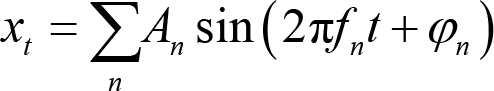
Spectral analysis is the basis of further analysis, such as connectivity analysis and spatial network analysis. A popular method for doing the spectral analysis is the Fourier transform, which decomposes the time‐series signal x_t to the sum of a set of sine waves (Panel A of Fig. 2):

x_{t} = \sum_{n} A_{n} \sin (2 π f_{n} t + φ_{n})

Fig. 2.

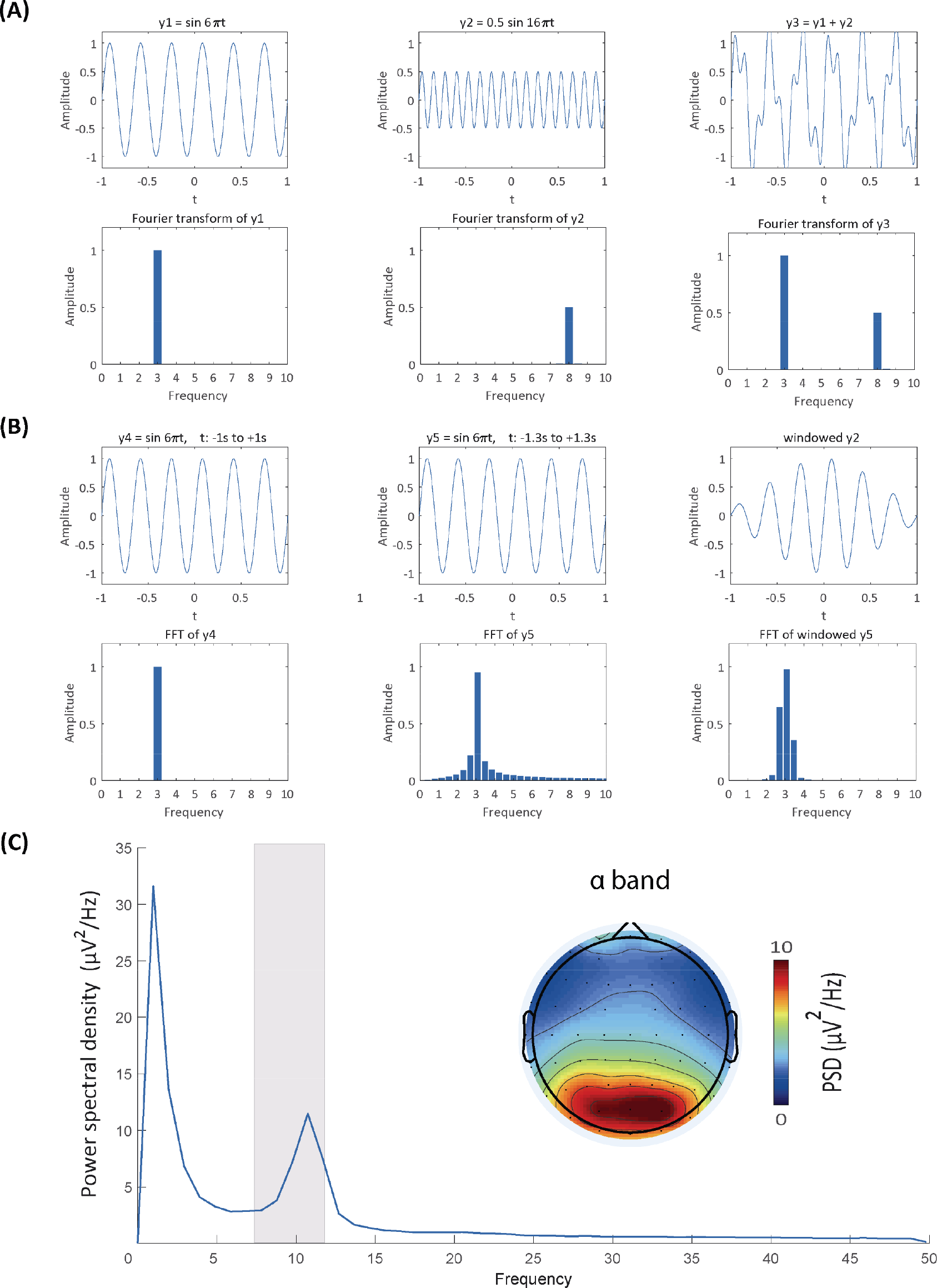
Spectral analysis. (A) Comparisons between the original signals and their frequency representations. The Fourier transform retains frequency and amplitude information of perfect sine waves (the first two columns) and the sum of two sine waves (the third column). (B) Frequency leakage from the fast Fourier transform (FFT) and windowing. Frequency leakage occurs when the signal does not have an integer number of cycles (the first vs. second column), but can be remedied by windowing the signal (the final column). (C) Power spectrum at Pz and topographic distribution of resting‐state EEG data. The grey rectangle indicates the power spectral density of the α frequency band, whose topographic distribution is shown in the topography.

where A_n is the amplitude, f_n is the frequency, and φ_n is the phase. Since EEG is sampled at discrete time points, it is more appropriate to perform a discrete Fourier transform. The Fourier coefficient X(k) for the EEG signal x(n) (n = 1, 2,…, N) is calculated as:

X (k) = \sum_{n = 0}^{N - 1} x (n) e^{- i 2 π k n / N}

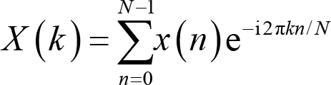
where k is the frequency localization and i the imaginary unit [43]. The frequency location is used to derive the frequency information,

f = \frac{k F_{s}}{N}

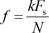
where F _s is the sampling rate, and N is the number of time points. Note that the smallest frequency we can extract is 0 Hz, and the largest frequency is half of the sampling frequency, which we term as the Nyquist frequency. X(k) is a series of complex numbers. The absolute value of X(k) normalized by the number of data points is the amplitude or magnitude of the corresponding sine wave, and the angle between the real part and imaginary part is the phase. That is,

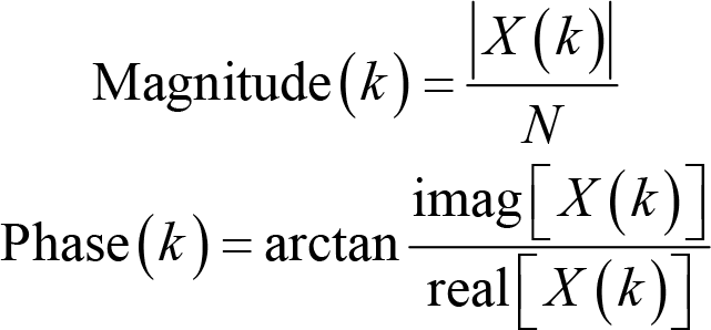
\begin{array}{r} Magnitude (k) = \frac{| X (k) |}{N} \\ Phase (k) = \arctan \frac{imag [X (k)]}{real [X (k)]} \end{array}

where imag[X(k)] and real[X(k)] are the imaginary and real part of X(k), respectively. The unit of magnitude is μV. With these two pieces of information, we can reconstruct the sine waves in the familiar form of the sine function. Apart from magnitude and phase, power is another oft‐used measure, which is defined as the squared magnitude:

Power (k) = {[\frac{| X (k) |}{N}]}^{2}

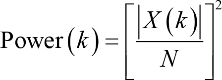
Apparently, the unit of power is μV². A derived measure from power is power spectral density (PSD),

PSD (k) = \frac{| X (k) |^{2}}{F_{s} N}

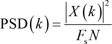
where F _s is the sampling rate. The unit is μV²/Hz.

In practice, to improve the calculation efficiency, we can use the fast Fourier transform (FFT) algorithm [44]. In the FFT, the number of sample points N is usually set to be a power of 2 to boost the computation speed. This condition is rarely satisfied in real life but can be compromised by adding zeros at both ends of the original time‐series, a process called “zero padding”.

3.1.2 Practical issues

(1) What is the correct scalar for magnitude, power, and PSD?

When doing the Fourier transform, we often find ourselves in an un expected situation where the magnitude is smaller than we would have expected if we calculate it with the formula introduced above. To be precise, the magnitude is one half of what it should have been. This is because we have omitted negative frequency parts, which mirror positive frequency responses in EEG data. In practice, we can safely ignore the issue of negative frequency and double the magnitude to fully recover the magnitude of the original signals. That is,

{Magnitude}^{'} (k) =2 \frac{| X (k) |}{N}

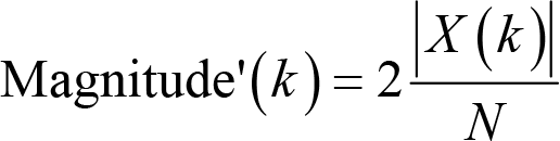
The same approach also applies to power and PSD

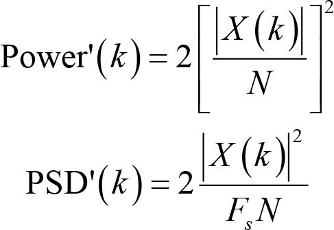
\begin{array}{l} {Power}^{'} (k) = 2 {[\frac{| X (k) |}{N}]}^{2} \\ {PSD}^{'} (k) = 2 \frac{| X (k) |}{F_{s} N} \end{array}

Note that doubling these measures will have little impact on most statistical tests since they are invariant under linear transformations. The only difference they make is that the descriptive statistics, for example, means and standard deviations, are twice the results calculated with formulas we introduced above.

(2) Why are there extra frequency responses?

Another unwanted consequence from the Fourier transform is that the frequency representation of a perfect sine wave somehow contains more information than the sine wave itself. (The readers may compare the first two columns in Panel B of Fig. 2). That is, the original frequency response is “leaked” to its adjacent frequencies. This leakage comes from the fact that the original signal is of limited duration and that the Fourier transform implicitly assumes that the signal repeats itself indefinitely [36]. If the signal does not have an integer number of cycles (the second column in Panel B of Fig. 2), repeating them would cause discontinuities at the edges, which leads to the smearing of frequency responses.

To minimize the influence of leakage, we taper the edges of the data with a window function (the third column in Panel B of Fig. 2). Typical window functions include Hann (sometimes called Hanning), Hamming, and Gaussian windows. The Hann window is preferred since it, by definition, tapers the data to zero at its both sides, eliminating edge discontinuities altogether [8]. However, tapering signals with window functions also leads to data loss at the edges. The Welch’s method can reduce the amount of data lost in windowing since the windows overlap in this method [45]. The best way to minimize data loss is certainly to apply to the data a rectangular window, the value within which is constantly 1. Indeed, the rectangular window is equivalent to leaving the data as they are without applying any window function. However, the problem of frequency leakage is totally ignored in this case.

(3) Why do we create segments for resting‐state EEG?

When addressing the topic of preprocessing, we mentioned that the resting‐state EEG is segmented even though it is possible to analyze the continuous EEG resting‐state data. The reasons for this procedure are that the spectrum for long continuous datasets often exhibits considerable variability, and that spectral peaks may not be clearly observed and precisely located. Dividing the entire data into multiple segments and averaging their spectra help reduce variability and obtain smoother results [46]. An alternative approach, called Welch’s method, is to allow segments to overlap a bit to reduce data loss due to windowing (see the last practical issue we have talked about) [45]. The amount of overlapping is up to the analyzers, though 50% overlapping is common. The number of segments is important as the procedure involves averaging. Some researchers suggest that there should be at least 10 segments (ideally 30 or more) [36].

(4) How can we visualize the results?

A graph typically illustrates how one variable is related to other variables. For spectral analysis, we have spectral estimates at every frequency bin and electrode of interest, so we can get the PSD (or magnitude, power) of an electrode by putting the frequency variable at the x axis and the spectral variable at the y axis (Panel C of Fig. 2). The topographic distributions of PSD in certain frequency bands may reflect underlying neurophysiological mechanisms and functions. We can thus cluster frequencies into frequency bands, take the mean PSD values, and plot their scalp topographies (Panel C of Fig. 2).

We should pay special attention to the scale of PSD in a graph. Two scales are available, namely linear and logarithm, which highlight different parts of the results and should accord with our purpose of visualization. Specifically, the linear scale (μV²/Hz) highlights the low‐frequency peaks and makes other spectral components less distinguishable, especially those in the extreme high‐frequency bands. On the other hand, the logarithmic scale [10log₁₀(μV²/Hz), or dB] renders spectral components of different frequency bands more visually comparable, though the spectral peaks cannot stand out. If we want to examine EEG spectral power over a wide range of frequency, the logarithmic scale may be more useful.

3.2 Connectivity Analysis

Effective communication between brain regions is indispensable for most cognitive functions [47]. Abundant evidence suggests that abnormalities of inter‐regional neural communication are associated with brain diseases, such as epilepsy [48], Alzheimer’s disease [49], and Parkinson’s disease [50]. Therefore, connectivity analysis is an important part of cognitive neuroscience studies.

In substance, all connectivity measures are based on statistical interdependence between signals [51]. The Pearson’s correlation coefficient between EEG signals of two or more electrodes is the simplest measure of connectivity, though rarely used in practice. In this section, we introduce two categories of connectivity measures: coherence and phase synchronization-based measures.

3.2.1 Coherence

Coherence is a widely adopted measure in EEG connectivity studies to assess the linear relationship between two signals at each frequency bin being evaluated [52]. To calculate the coherence between two electrodes a and b, we Fourier transform the signals at these electrodes and compute the coherence as:

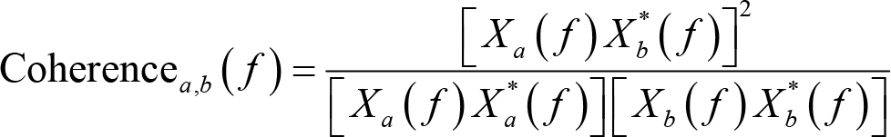
{Coherence}_{a, b} (f) = \frac{{[X_{a} (f) X_{b}^{*} (f)]}^{2}}{[X_{a} (f) X_{a}^{*} (f)] [X_{b} (f) X_{b}^{*} (f)]}

where X_a ( f ) is the Fourier coefficients for signals at electrode a, f is the frequency location, and $X_{b}^{*} (f)$ is the complex conjugate of X_a ( f ). The complex conjugate of a complex number a + bi is a – bi. Coherence ranges over [0, 1], with a larger value suggesting stronger statistical dependence between two signals.

3.2.2 Phase synchronization‐based measures

As introduced in 3.1.1 The Fourier transform, phase is the angle between the real part and imaginary part of the Fourier coefficients. It provides irreplaceable information in various EEG connectivity measures. Apart from the FFT, many other methods exist to extract the phase information, such as the short‐time Fourier transform, continuous wavelet transform, and band‐pass filtering combined with the Hilbert transform. The phase synchronization between two signals independent of the amplitudes of the respective signals can be quantified by phase‐locking value (PLV) [53, 54]. Formally, PLV is computed using the following equation:

PLV (f) = | \frac{1}{M} \sum_{m = 1}^{M} e^{i (φ_{a, m} - φ_{b, m})} |

where f is a given frequency, M is the number of trials, φ_a _,m and φ_b _,m are the phase angles on trial m from electrode a and b, respectively. Intuitively, PLV is the absolute value of the averaged complex polar representation of phase angles. PLV ranges over [0, 1]. A larger PLV implies stronger connectivity. The distribution range of the phase difference series is [0, 2π). A PLV of 0 indicates a random distribution of phase differences, whereas a PLV of 1 means that the phase difference is constant.

However, the connectivity assessed by PLV is spurious if activities from electrodes a and b are generated by a common source. Theoretically, the common source would lead to a phase angle difference of zero or π between two electrodes, making the PLV equal to 1 even though there is no functional connectivity whatsoever between these electrodes. To address this problem, we can use another phase‐based connectivity measure, phase lag index (PLI) [55], which is defined as:

PLI (f) = | \frac{1}{M} \sum_{m = 1}^{M} sign (φ_{a, m} - φ_{b, m}) |

where f is a given frequency, sign() is the sign function, which equals −1 for negative inputs, 0 for zero, 1 for positive inputs. The range of PLI value is also [0, 1], with 1 indicating perfect phase locking at a value different from 0 or π, that is, a strong coupling and connection relationship. A PLI of 0 means no coupling or coupling with a phase difference centered around 0 or π. However, this measure is also imperfect, as it may not capture linear but functionally meaningful interactions [56]. An improved measure is the weighted phase lag index (wPLI) [57], which is defined as:

wPLI (f) = \frac{M^{- 1} \sum_{m = 1}^{M} | imag [X_{a} (f) X_{b}^{*} (f)] | sign (φ_{a, m} - φ_{b, m})}{M^{- 1} \sum_{m = 1}^{M} imag | [X_{a} (f) X_{b}^{*} (f)] |}

where f is a given frequency, X_a ( f ) is the Fourier coefficients for signals at electrode a, $X_{a}^{*} (f)$ is the complex conjugate of X_a ( f ), and imag() takes the imaginary part of a complex number.

In practice, we often perform the band‐pass filtering before extracting the spectra of signals to compute the PLV, PLI, and wPLI.

3.2.3 Practical issues

(1) Which measures should we use?

We have introduced four measures of connectivity (or five, if we consider the Pearson’s correlation) above, but there are actually more connectivity measures. A natural question that follows is which one we should select. The answer depends on the strengths and weaknesses of these measures, and whether we are doing hypothesis- or data‐driven analysis.

Though widely used, coherence suffers from the common source problem, is influenced by magnitudes of signals, and is unable to detect nonlinear relationships [24, 58]. The common source problem also plagues PLV. On the other hand, PLI and wPLI are largely immune to this thorny problem. The weakness of PLI is that this index is insensitive to the amount of phase clustering, but is sensitive to additional uncorrelated noise [57]. wPLI is less noise-sensitive than PLI, but is unable to reliably separate contributions of amplitude and phase to connectivity [57].

The way we do our analysis also has an impact on the choice of connectivity measures. Among them, PLV might be most sensitive to detecting connectivity [8]. As a result, if we have a strong hypothesis to test, PLV provides a stronger statistical power. To avoid the common source problem, we should also test our PLV results against the potential influence of common sources [8]. However, if we are intent to do data‐driven or exploratory analysis, the common source problem outweigh the statistical power, and PLI and wPLI appear more appropriate. (2) Do these four measures imply causal relationships?

No. The four measures we have talked about assess statistical interdependence between signals, not their causal relationship. This kind of connectivity is called functional connectivity. Interdependence between two signals, x and y, can be interpreted in at least four ways. First, x is the cause of y; second, y is the cause of x; third, x and y have a common cause c; fourth, x and y are the causes of the common fixed effect e [59]. Without further information, we can never determine which one of these interpretations is correct. Some connectivity measures like Granger causality [60] are presumed to establish a causal relationship, but actually, neither establish nor even require causality [8]. To reveal a causal relationship, we appeal to randomized experiments and/or sophisticated statistical techniques controlling confounding factors [59]. Therefore, we recommend that connectivity always be explained in terms of interdependence.

(3) Can we do connectivity analysis at a level other than electrodes?

Yes. Connectivity analysis can also be conducted at the source level. In fact, source connectivity is more interpretable than electrode connectivity, since the former can be intuitively understood as communications between brain regions. However, we have to estimate the source‐localized activities (i.e., current source density) in the brain before performing connectivity analysis at the source level [61]. We then extract activities in regions of interest according to brain atlases and calculate connectivity measures that we have introduced. It is noteworthy that source connectivity relies heavily on the SNR of the data and the accuracy of source localization, both of which are unsatisfactory in typical EEG data.

(4) How can we visualize the results?

In resting‐state EEG, connectivity at the electrode level is a function of frequency bins and electrode pairs. Two primary sorts of graphs are thus available: one shows how connectivity varies across electrodes (Panel A of Fig. 3), while the other depicts statistically significant connectivity of certain frequency bands for every electrode pairs on a topographical map (Panel B of Fig. 3). Due to the huge number of possible electrode pairs, the multiple comparison problem becomes extremely serious in the latter type of graph. We thus need to control the Type I error rate with methods like the false discovery rate or network‐based statistic.

Fig. 3.

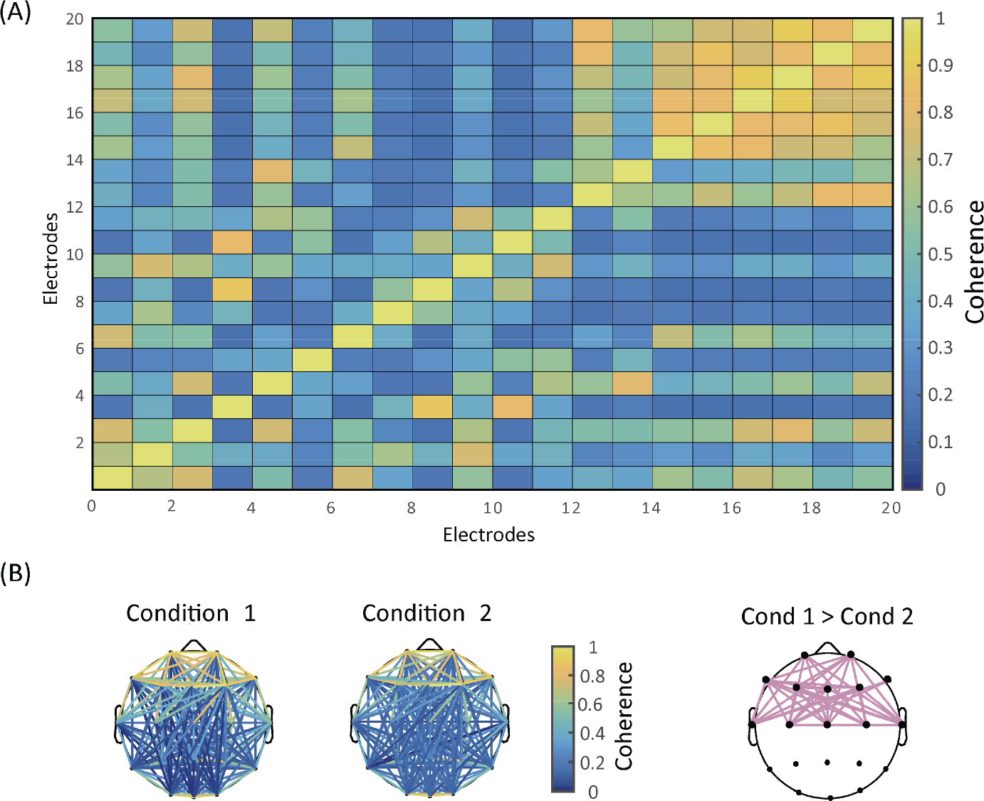
Connectivity analysis. (A) Results of electrode‐wise coherence. (B) Topographic distributions of coherence. The first two columns show coherence topographies for two different conditions. The last column displays the electrode pairs where the coherence of Condition 1 is statistically larger than that of Condition 2.

3.3 Microstate analysis

3.3.1 Basic ideas

Developed in the 1980s, microstate analysis is a relatively new technique that fully utilizes the rich spatial information of EEG signals [62]. Topographic maps of resting‐state EEG do not vary randomly over time, but exhibit several fixed patterns called microstates, each of which typically lasts for 100 milliseconds or so [62, 63]. With merely 4–8 distinct microstates, we can explain approximately 80% of the variance in resting‐state EEG data [63]. Four microstate classes have been consistently identified across resting‐state EEG studies [64].

Functionally, microstate analysis provides us a window to brain network dynamics on a millisecond timescale [65]. Microstates are related to the activity of resting‐state brain networks in fMRI [66] and likely to reflect ongoing mental processes [62]. Please note that microstate analysis can also be applicable to task‐related EEG, in which microstates in ERP waveforms may reflect specific ERP components [53].

To do microstate analysis, we first measure global brain activity and then cluster topographic maps.

3.3.2 Measuring global brain activity

Global brain activity can be assessed by three measures: global field power (GFP), global map dissimilarity (GMD), and spatial correlation [67]. Specifically, GFP is defined as the standard deviation of the electrical potentials over all electrodes at each time point [68], that is:

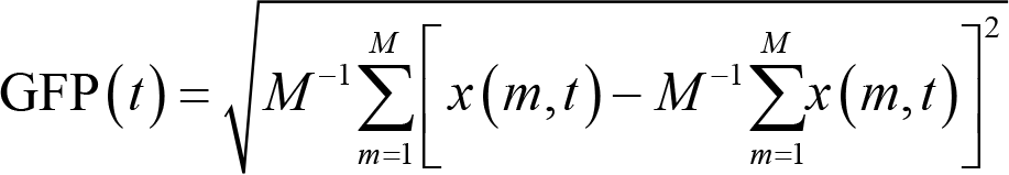
GFP (t) = \sqrt{M^{- 1} \sum_{m = 1}^{M} {[x (m, t) - M^{- 1} \sum_{m = 1}^{M} x (m, t)]}^{2}}

where x(m,t) is the potentials of electrode m at the given time point t, and M is the number of electrodes. Note that GFP is reference‐independent as a result of the mathematical properties of standard deviation [67]. A large GFP is associated with a high topographic SNR and a relatively stable topographic configuration. On the other hand, a small GFP indicates a low SNR and changing topographic maps.

GMD is an index of configuration differences between two topographic maps, u and v [69]. These two maps can be in different conditions at the same time point or in the same condition but at two different time points. Formally, GMD is defined as:

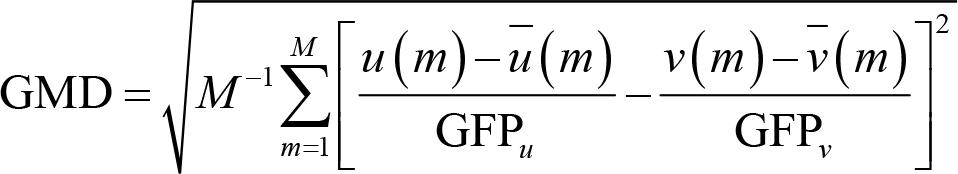
GMD = \sqrt{M^{- 1} \sum_{m = 1}^{M} {[\frac{u (m) - \bar{u} (m)}{{GFP}_{u}} - \frac{v (m) - \bar{v} (m)}{{GFP}_{v}}]}^{2}}

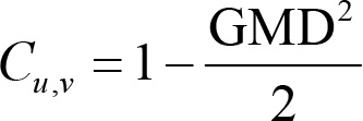
where u(m) and v(m) are the potentials of electrode m in two different maps, $\bar{u} (m)$ and $\bar{v} (m)$ are the average potentials of all electrodes, GFP _u and GFP _v are the respective GFPs, and M is the number of electrodes. A measure directly related to GMD is spatial correlation:

C_{u, v} = 1 - \frac{{GMD}^{2}}{2}

The range of spatial correlation is [−1, 1]. 1 means that the two maps are equal after being normalized by the respective GFP, whereas −1 indicates that the two GFP‐normalized maps have the same topographic distribution with reversed polarity. Note GMD and GFP, as well as spatial correlation and GMD, are negatively correlated. Therefore, scalp potential maps remain quasi‐stable when spatial correlation is high [69].

3.3.3 Clustering topographic maps

After measuring the global brain activity, we group all the topographic maps into a small set of classes, regardless of the order of their appearances, with clustering algorithms. Here, a popular algorithm is k‐means clustering that works as follows [67]. First, compute GFP for every topographic map and choose those at the GFP peaks as the “original maps”. Second, select n “template maps” randomly from those original maps. Third, calculate the pairwise spatial correlation between template maps and original maps. Global explained variance (GEV) can be calculated for template maps to assess how well they describe original maps. GEV is defined as:

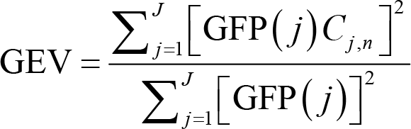
GEV = \frac{\sum_{j = 1}^{J} {[GFP (j) C_{j, n}]}^{2}}{\sum_{j = 1}^{J} {[GFP (j)]}^{2}}

where GFP(j) is the GFP for original map j, C_j,n is the spatial correlation between original map j and template map n, and J is the number of original maps. For any original map, there will be, among all the n template maps, only one template map whose spatial correlation with this original map is the largest. In other words, one or more original maps will have the largest spatial correlation with a specific template map. Fourth, update each template map by averaging original maps that have the largest spatial correlation with this template map. Fifth, reiterate the third and fourth steps until GEV achieves stability.

Note that the initial n template maps should be defined before clustering. We can repeat the whole procedure time and again until the highest GEV is obtained. Of course, this is somewhat unrealistic since the number of all possible combinations of n template maps can be prohibitively large. A simple solution is to determine a number a priori for these random selections. The set of template maps with the largest GEV in these selections are retained. Also, the number of template maps (n) is chosen arbitrarily. We can repeat the above steps with n + 1, n + 2,…, n + i template maps until the number is equal to that of original maps. Additional criteria, such as the cross‐validation criterion and the Krzanowski‐Lai criterion, can help us determine the optimal number of template maps, which is interpreted as the number of clusters we want to identify [70]. As mentioned above, four clusters are appropriate for resting‐state EEG in most previous studies [64].

To quantitatively describe the dynamic changes of brain states, we can rely on four parameters: (1) the average duration of a microstate class, (2) occurrence frequency per second of a microstate class, (3) time coverage of a microstate class, and (4) the transition probability between adjacent microstate classes [62, 71].

3.3.3 Practical issues

(1) Is there any specific tool for doing microstate analysis?

Microstate analysis is computationally demanding. Fortunately, there are several specific tools open‐accessible for microstates analysis: the LORETA software, the EEGLAB plugin, and the Cartool software. They can be downloaded from the following websites:

LORETA: http://www.uzh.ch/keyinst/loreta.htm EEGLAB plugin: https://sccn.ucsd.edu/wiki/EEGLAB_Extensions_and_plugins

Cartool: https://sites.google.com/site/fbmlab/cartool

(2) How can we visualize the results?

In microstates analysis, GFP waveforms and topographic maps are imperative. GFP waveforms depict how GFP values vary with time. At every time point, we can draw the topographic map, showing the spatial distribution of electric potentials across all electrodes. However, not all these maps have functional meaning in microstate analysis. Instead, we cluster topographic maps into several microstates that explain most variances in resting‐state EEG data and then draw topographic maps corresponding to the microstates we obtained (Fig. 4).

Fig. 4.

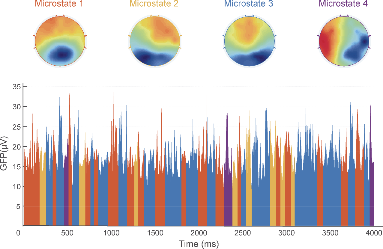
Microstate analysis. The first row shows four microstates extracted from the data. The second row exhibits the waveform of global field potentials (GFP) and the temporal distribution of the four microstates, indicated by four different colors corresponding to the colors of the titles “Microstate 1–4” in the first row.

3.4 Advanced techniques

In addition to the basic methods described above, there are various advanced methods that could be utilized to understand EEG data better. Below we briefly introduce a few of them, including nonlinear neural dynamics, complex network, and machine learning.

3.4.1 Nonlinear neural dynamics

EEG signals are the output of the brain, an enormously complex biological system with typical nonlinear dynamic properties [72, 73]. Therefore, it is helpful to apply nonlinear neural dynamics methods to capture EEG dynamics and disclose their underlying neural processes. Complexity and entropy are commonly used measures to extract EEG nonlinear characteristics. Complexity measures the degree of randomness in time series [74]. Entropy measures the distribution of probability characteristics of the signal based on Shannon information theory [75].

3.4.2 Complex networks

The brain can be regarded as a complex network due to its complex structure and function. As a result, quantifying the network characteristics of the brain can help us understand its inherent complex interrelations and information flow. In EEG analysis, we can conduct two types of complex network analysis: spatial complex network analysis and temporal complex network analysis.

Complex network analysis is based on graph theory, in which the structure of a complex network can be represented by an abstract topological graph comprised of a series of nodes and edges between nodes [76, 77]. Key features of the network topography are degree, characteristic path length, clustering coefficient, and betweenness centrality [78, 79]. Specifically, the degree of a node is the number of nodes connected to it; the characteristic path length of two nodes refers to the shortest length of the path between them; the clustering coefficient of a node is defined as the ratio of the number of edges between a node of interest and the nodes connected to it to the total number of edges between all those nodes; the betweenness of a node is the number of shortest paths through the node.

3.4.3 Machine learning

Theoretically, if there is a mapping between mental states and brain states in some context, then it must be possible to infer the specific mental state from the brain state. However, neural data representing brain states are high dimensional and noisy. Traditional statistical models like regression do not work very well for such high dimensional datasets. In contrast, machine learning is capable of making full use of multitudinous available features to decode brain states [80]. As a result, this technique has become an increasingly popular advanced technique to search for the neural correlates of mental states [12, 81].

In EEG analysis, machine learning extracts useful information from high‐dimensional EEG data, decodes and characterizes the diverse states of the brain, and finally discriminates these distinct states [81]. Machine learning analysis includes steps of feature extraction and selection, training, classifier choice, result evaluation, and pattern expression [80]. Specifically, in EEG analysis, we extract features about EEG signal, define the class (e.g., experimental conditions about cognitive or perceptual responses), organize the feature samples into a training sample and a test sample, and give class labels to the training sample. We then choose a suitable classifier and apply it to the training sample, and eventually use the test sample to make an evaluation of classifier performance.

4 Concluding remarks

EEG is an old but powerful technique for understanding the neural implementation of mental processes. In this review, we introduce some of the basic and advanced signal processing methods for resting‐state EEG to make full use of temporal and spatial information of the data. The Fourier transform extracts the frequency‐domain measures, such as magnitude, power, and PSD, and produces information to compute connectivity measures, like coherence, PLV, PLI, and wPLI. Spatial distribution of the signals across the scalp helps define GFP, GMD, spatial correlation, and GEV to cluster topographical maps and generate microstates. With the help of these methods, we can extract meaningful electrophysiological measures that might be associated with specific psychological functions in a given context.

It is important that not all EEG measures are necessary for a single study. On the contrary, abusing these measures can be detrimental, especially when they add little or no new knowledge about the psychological processes that we are investigating. Proper use of EEG signal processing methods ensures that we could exploit the power of the EEG technique to gain valuable insights into how the mind actually works in the brain.

Footnotes

Conflict of interests

The authors have declared that no competing interests exist.

Acknowledgment

This work was supported by the National Natural Science Foundation of China (Grant No. 31822025, No. 31671141). The funders had no role in study design, data collection and analysis, decision to publish, or preparation of the manuscript.

References

Gerrig

. Psychology and Life. 20th ed. Boston, USA: Pearson, 2013.

Caton

. Electrical currents of the brain. Br Med J. 1875, 2: 278.

Berger

. Über das Elektrenkephalogramm des Menschen. Archiv F Psychiatrie. 1937, 106(1): 577–584.

Luck

. An Introduction to the Event-Related Potential Technique. 2nd ed. Cambridge, MA, USA: MIT Press, 2014.

Adrian

Matthews

BHC

. The Berger rhythm: potential changes from the occipital lobes in man. Brain. 1934, 57(4): 355–385.

Jasper

Carmichael

. Electrical potentials from the intact human brain. Science. 1935, 81(2089): 51–53.

Gibbs

Davis

Lennox

. The electroencephalogram in epilepsy and in conditions of impaired consciousness. Arch NeurPsych. 1935, 34(6): 1133–1148.

Cohen

MX.

Analyzing Neural Time Series Data: Theory and Practice. Cambridge, MA, USA: MIT Press, 2014.

Xia

. EEG: neural basis and measurement. In EEG Signal Processing and Feature Extraction Hu

Zhang

, Eds. Singapore: Springer Singapore, 2019.

10.

Murakami

Okada

. Contributions of principal neocortical neurons to magnetoencephalography and electroencephalography signals. J Physiol. 2006, 575(pt 3): 925–936.

11.

Logothetis

. The underpinnings of the BOLD functional magnetic resonance imaging signal. J Neurosci. 2003, 23(10): 3963–3971.

12.

Iannetti

. Neural indicators of perceptual variability of pain across species. Proc Natl Acad Sci USA. 2019, 116(5): 1782–1791.

13.

Ploner

May

. EEG and MEG in pain research - Current state and future perspectives. Pain. 2017, 159(2): 206.

14.

Romei

Gross

Thut

. On the role of prestimulus alpha rhythms over occipito-parietal areas in visual input regulation: correlation or causation? J Neurosci. 2010, 30(25): 8692–8697.

15.

Tomassini

Spinelli

Jacono

, et al. Rhythmic oscillations of visual contrast sensitivity synchronized with action. J Neurosci. 2015, 35(18): 7019–7029.

16.

Wöstmann

Alavash

Obleser

. Alpha oscillations in the human brain implement distractor suppression independent of target selection. J Neurosci. 2019, 39(49): 9797–9805.

17.

Vogel

McCollough

Machizawa

. Neural measures reveal individual differences in controlling access to working memory. Nature. 2005, 438(7067): 500–503.

18.

Polanía

Krajbich

Grueschow

, et al. Neural oscillations and synchronization differentially support evidence accumulation in perceptual and value-based decision making. Neuron. 2014, 82(3): 709–720.

19.

Weiss

Mueller

. The contribution of EEG coherence to the investigation of language. Brain Lang. 2003, 85(2): 325–343.

20.

Dennis

Solomon

. Frontal EEG and emotion regulation: electrocortical activity in response to emotional film clips is associated with reduced mood induction and attention interference effects. Biol Psychol. 2010, 85(3): 456–464.

21.

Hehman

Volpert

Simons

. The N400 as an index of racial stereotype accessibility. Soc Cogn Affect Neurosci. 2014, 9(4): 544–552.

22.

Cameron

Payne

Sinnott-Armstrong

, et al. Implicit moral evaluations: a multinomial modeling approach. Cognition. 2017, 158: 224–241.

23.

Snyder

Raichle

. A brief history of the resting state: the Washington University perspective. Neuroimage. 2012, 62(2): 902–910.

24.

Babiloni

Barry

Başar

, et al. International Federation of Clinical Neurophysiology (IFCN) - EEG research workgroup: Recommendations on frequency and topographic analysis of resting state EEG rhythms. Part 1: Applications in clinical research studies. Clin Neurophysiol. 2020, 131(1): 285–307.

25.

Grandy

Werkle-Bergner

Chicherio

, et al. Individual alpha peak frequency is related to latent factors of general cognitive abilities. Neuroimage. 2013, 79: 10–18.

26.

Peng

. EEG preprocessing and denoising. In EEG Signal Processing and Feature Extraction Hu

Zhang

, Eds. Singapore: Springer Singapore, 2019.

27.

Delorme

Makeig

. EEGLAB: an open source toolbox for analysis of single-trial EEG dynamics including independent component analysis. J Neurosci Methods. 2004, 134(1): 9–21.

28.

Lai

Valdes-Sosa

, et al.

How do reference montage and electrodes setup affect the measured scalp EEG potentials?

J Neural Eng. 2018, 15(2): 02601 3.

29.

Pivik

Broughton

Coppola

, et al. Guidelines for the recording and quantitative analysis of electroencephalographic activity in research contexts. Psychophysiology. 1993, 30(6): 547–558.

30.

Yao

Qin

, et al.

Which reference should we use for EEG and ERP practice?

Brain Topogr. 2019, 32(4): 530–549.

31.

Dien

Issues in the application of the average reference: Review, critiques, and recommendations. Behav Res Methods Instruments Comput. 1998, 30(1): 34–43.

32.

Junghöfer

Elbert

Tucker

, et al. The polar average reference effect: a bias in estimating the head surface integral in EEG recording. Clin Neurophysiol. 1999, 110(6): 1149–1155.

33.

Teplan

. Fundamentals of EEG measurement. Meas Sci Rev. 2002, 2(2): 1–11.

34.

Yao

. A method to standardize a reference of scalp EEG recordings to a point at infinity. Physiol Meas. 2001, 22(4): 693–711.

35.

Yao

Wang

Oostenveld

, et al. A comparative study of different references for EEG spectral mapping: the issue of the neutral reference and the use of the infinity reference. Physiol Meas. 2005, 26(3): 173–184.

36.

Freeman

Quiroga

. Imaging brain function with EEG. New York, NY, USA: Springer New York, 2013.

37.

Greischar

Burghy

van Reekum

, et al. Effects of electrode density and electrolyte spreading in dense array electroencephalographic recording. Clin Neurophysiol. 2004, 115(3): 710–720.

38.

Zou

Nathan

Jafari

. Automatic identification of artifact-related independent components for artifact removal in EEG recordings. IEEE J Biomed Health Inform. 2016, 20(1): 73–81.

39.

Makeig

Debener

Onton

, et al. Mining event-related brain dynamics. Trends Cogn Sci. 2004, 8(5): 204–210.

40.

Chaumon

Bishop

Busch

. A practical guide to the selection of independent components of the electroencephalogram for artifact correction. J Neurosci Methods. 2015, 250: 47–63.

41.

Kane

Acharya

Benickzy

, et al. A revised glossary of terms most commonly used by clinical electroencephalographers and updated proposal for the report format of the EEG findings. Revision 2017. Clin Neurophysiol Pract. 2017, 2: 170–185.

42.

Nunez

Srinivasan

. Electric Fields of the Brain. 2nd ed. New York, USA: Oxford University Press, 2006.

43.

Zhang

. Spectral and time-frequency analysis. In EEG Signal Processing and Feature Extraction Hu

Zhang

, Eds. Singapore: Springer Singapore, 2019.

44.

Cooley

Tukey

. An algorithm for the machine calculation of complex Fourier series. Math Comp. 1965, 19(90): 297.

45.

Welch

. The use of fast Fourier transform for the estimation of power spectra: a method based on time averaging over short, modified periodograms. IEEE Trans Audio Electroacoustics. 1967, 15(2): 70–73.

46.

Bartlett

MS.

An Introduction to Stochastic Processes: with Special Reference to Methods and Applications. 3rd ed. Cambridge, MA, USA: Cambridge University Press, 1978.

47.

Abrams

Lynch

Cheng

, et al. Underconnectivity between voice-selective cortex and reward circuitry in children with autism. Proc Natl Acad Sci USA. 2013, 110(29): 12060–12065.

48.

Ibrahim

Anderson

Akiyama

, et al. Neocortical pathological high-frequency oscillations are associated with frequency-dependent alterations in functional network topology. J Neurophysiol. 2013, 110(10): 2475–2483.

49.

Dubovik

Bouzerda-Wahlen

Nahum

, et al. Adaptive reorganization of cortical networks in Alzheimer’s disease. Clin Neurophysiol. 2013, 124(1): 35–43.

50.

Fogelson

, et al. Functional connectivity abnormalities during contextual processing in schizophrenia and in Parkinson’s disease. Brain Cogn. 2013, 82(3): 243–253.

51.

Aertsen

Gerstein

Habib

, et al. Dynamics of neuronal firing correlation: modulation of “effective connectivity”. J Neurophysiol. 1989, 61(5): 900–917.

52.

Niso

Bruña

Pereda

, et al. HERMES: towards an integrated toolbox to characterize functional and effective brain connectivity. Neuroinformatics. 2013, 11(4): 405–434.

53.

Valentini

Zhang

, et al. The primary somatosensory cortex contributes to the latest part of the cortical response elicited by nociceptive somatosensory stimuli in humans. Neuroimage. 2014, 84: 383–393.

54.

Lachaux

Rodriguez

Martinerie

, et al. Measuring phase synchrony in brain signals. Hum Brain Mapp. 1999, 8(4): 194–208.

55.

Stam

Nolte

Daffertshofer

. Phase lag index: assessment of functional connectivity from multi channel EEG and MEG with diminished bias from common sources. Hum Brain Mapp. 2007, 28(11): 1178–1193.

56.

van Diessen

Numan

van Dellen

, et al. Opportunities and methodological challenges in EEG and MEG resting state functional brain network research. Clin Neurophysiol. 2015, 126(8): 1468–1481.

57.

Vinck

Oostenveld

van Wingerden

, et al. An improved index of phase-synchronization for electrophysiological data in the presence of volume-conduction, noise and sample-size bias. Neuroimage. 2011, 55(4): 1548–1565.

58.

Blinowska

. Review of the methods of determination of directed connectivity from multichannel data. Med Biol Eng Comput. 2011, 49(5): 521–529.

59.

Pearl

Glymour

Jewell

. Causal Inference in Statistics: A Primer. Chichester, UK: Wiley, 2016.

60.

Granger

CWJ

. Investigating causal relations by econometric models and cross-spectral methods. Econometrica. 1969, 37(3): 424–438.

61.

Jia

. Connectivity analysis. In EEG Signal Processing and Feature Extraction Hu

Zhang

, Eds. Singapore: Springer Singapore, 2019.

62.

Lehmann

Ozaki

Pal

. EEG alpha map series: brain micro-states by space-oriented adaptive segmentation. Electroencephalogr Clin Neurophysiol. 1987, 67(3): 271–288.

63.

Pascual-Marqui

Michel

Lehmann

. Segmentation of brain electrical activity into microstates: model estimation and validation. IEEE Trans Biomed Eng. 1995, 42(7): 658–665.

64.

Lehmann

Pascual-Marqui

Michel

. EEG microstates. Scholarpedia. 2009, 4(3): 7632.

65.

Khanna

Pascual-Leone

Michel

, et al. Microstates in resting-state EEG: current status and future directions. Neurosci Biobehav Rev. 2015, 49: 105–113.

66.

Britz

Van De Ville

Michel

. BOLD correlates of EEG topography reveal rapid resting-state network dynamics. Neuroimage. 2010, 52(4): 1162–1170.

67.

Murray

Brunet

Michel

. Topographic ERP analyses: a step-by-step tutorial review. Brain Topogr. 2008, 20(4): 249–264.

68.

Lehmann

Skrandies

. Reference-free identification of components of checkerboard-evoked multichannel potential fields. Electroencephalogr Clin Neurophysiol. 1980, 48(6): 609–621.

69.

Brunet

Murray

Michel

. Spatiotemporal analysis of multichannel EEG: CARTOOL. Comput Intell Neurosci. 2011, 2011: 813870.

70.

Jia

. Microstate analysis. In EEG Signal Processing and Feature Extraction Hu

Zhang

, Eds. Singapore: Springer Singapore, 2019.

71.

Michel

Koenig

. EEG microstates as a tool for studying the temporal dynamics of whole-brain neuronal networks: a review. Neuroimage. 2018, 180(pt b): 577–593.

72.

Bai

Liang

. Nonlinear neural dynamics. In EEG Signal Processing and Feature Extraction Hu

Zhang

, Eds. Singapore: Springer Singapore, 2019.

73.

Sanei

Chambers

. EEG Signal Processing. West Sussex, UK: John Wiley & Sons, 2007.

74.

Lempel

Ziv

. On the complexity of finite sequences. IEEE Trans Inform Theory. 1976, 22(1): 75–81.

75.

Shannon

. A mathematical theory of communication. Bell Syst Tech J. 1948, 27(3): 379–423.

76.

Rubinov

Knock

Stam

, et al. Small-world properties of nonlinear brain activity in schizophrenia. Hum Brain Mapp. 2009, 30(2): 403–416.

77.

Trudeau

. Introduction to Graph Theory. 2nd ed. New York, USA: Dover Publications, 1994.

78.

Zhang

. EEG signal processing and feature extraction[M]. Singapore: Springer Singapore, 2019.

79.

Wen

Wei

Zhou

, et al.Spatial complex brain network. In EEG Signal Processing and Feature Extraction Hu

Zhang

, Eds. Singapore: Springer Singapore, 2019.

80.

. Machine learning. In EEG Signal Processing and Feature Extraction Hu

Zhang

, Eds. Singapore: Springer Singapore, 2019.

81.

Huang

Xiao

Hung

, et al. A novel approach to predict subjective pain perception from single-trial laser-evoked potentials. Neuroimage. 2013, 81: 283–293.

Demystifying signal processing techniques to extract resting-state EEG features for psychologists

Abstract

Keywords

1 Introduction

2 EEG Preprocessing

2.1 Re‐referencing

2.2 Filtering

2.3 Extracting Data Segments

2.4 Removing bad segments and interpolating bad electrodes

2.5 Removal of EEG artifacts using ICA

3 Resting‐state EEG processing

3.1 Spectral analysis

3.1.1 The Fourier transform

3.1.2 Practical issues

3.2 Connectivity Analysis

3.2.1 Coherence

3.2.2 Phase synchronization‐based measures

3.2.3 Practical issues

3.3 Microstate analysis

3.3.1 Basic ideas

3.3.2 Measuring global brain activity

3.3.3 Clustering topographic maps

3.3.3 Practical issues

3.4 Advanced techniques

3.4.1 Nonlinear neural dynamics

3.4.2 Complex networks

3.4.3 Machine learning

4 Concluding remarks

Footnotes

Conflict of interests

Acknowledgment

References