Sage Journals: Discover world-class research

Abstract

To investigate neural mechanisms of human psychology with electroencephalography (EEG), we typically instruct participants to perform certain tasks with simultaneous recording of their brain activities. The identification of task‐related EEG responses requires data analysis techniques that are normally different from methods for analyzing resting‐state EEG. This review aims to demystify commonly used signal processing methods for identifying task‐related EEG activities for psychologists. To achieve this goal, we first highlight the different preprocessing pipelines between task‐related EEG and resting‐state EEG. We then discuss the methods to extract and visualize event‐related potentials in the time domain and event‐related oscillatory responses in the time‐frequency domain. Potential applications of advanced techniques such as source analysis and single‐trial analysis are briefly discussed. We conclude this review with a short summary of task‐related EEG data analysis, recommendations for further study, and caveats we should take heed of.

Keywords

1 Introduction

Psychologists are particularly interested in revealing neural mechanisms of mental functions. Electroencephalography (EEG) is an increasingly popular, non‐invasive method to investigate how such functions are implemented in the human brain, due to its advantages in millisecond temporal resolution and financially acceptable costs. To achieve a better understanding of human mental functions, perplexing signal processing techniques are required to analyze EEG data and extract relevant EEG measures. To facilitate the applications of EEG techniques for psychologists, we introduce useful EEG signal processing techniques with MATLAB scripts (provided in the supplementary material) in two reviews.

We have extensively discussed the methods to analyze resting‐state EEG data in the previous review included in this special issue [1]. In this review, we focus on the techniques to analyze task‐related EEG data, where participants perform certain tasks while their brain activities are simultaneously recorded as EEG signals. To do so, we first highlight the importance of collecting high‐quality EEG data and describe the differences of preprocessing pipelines for task‐related EEG and resting‐state EEG. We then take a closer look at the techniques to extract event‐related potentials in the time domain and event‐related oscillatory responses in the time‐frequency domain (Fig. 1). Meanwhile, we briefly introduce the potential applications of some advanced techniques such as source analysis and single‐trial analysis. Finally, we conclude with a short summary of task‐related EEG techniques, recommendations for further study, and caveats that we should take heed of. Readers are strongly encouraged to first read relevant content in our review on methods for resting‐state EEG [1], where data preprocessing and the Fourier transform have been introduced with more details.

Fig. 1.

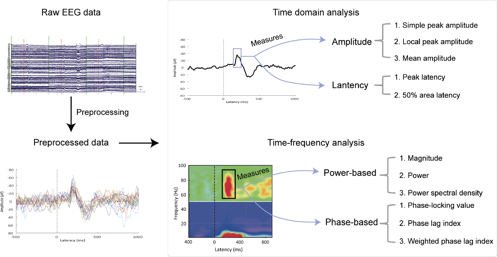
Overview of task‐related EEG data analysis. Raw EEG data are preprocessed to obtain the denoised data, on which time domain and time‐frequency analysis are performed. For time domain analysis, the amplitude and latency can be extracted to quantify the ERP waveform. Methods to measure the former include the simple peak amplitude, local peak amplitude, and mean amplitude; the latter can be measured using the peak latency method and 50% area latency method. For time‐frequency analysis, important measures include power‐based measures (magnitude, power, and power spectral density) and phase‐based measures (phase‐locking value, phase lag index, and weighted phase lag index).

2 EEG preprocessing

Besides neuronal activity, raw EEG data also contain physiological artifacts and non‐physiological noise. Therefore, the preprocessing of raw EEG data is crucial to denoise, remove artifacts, and ultimately improve the signal-to‐noise ratio (SNR) prior to further analysis. The preprocessing procedure for task‐related EEG is similar to that for resting‐state EEG (Table 1) [2], and their differences were highlighted in 2.2 Task‐related EEG preprocessing. Note that the steps in Table 1 are not applicable to all occasions. The study design, the nature of data, and the analysis techniques may impact the preprocessing procedure [2]. If necessary, the pipeline should be modified accordingly in practice.

Table 1.

Summary of preprocessing procedures for task‐related EEG data.

Order	Preprocessing procedures	Remarks
1	Filtering	High‐pass filter (e.g., 0.01–1 Hz)Low‐pass filter (e.g., 30–100 Hz)
2	Extracting epochs and baseline correction	Extract epochs using fix length (e.g., −200–800 ms)Remove baseline values (e.g., −200–0 ms)
3	Removing bad epochs and interpolating bad electrodes	Remove epochs with gross artifacts;Do not remove too many epochs (e.g., > 10%)
4	Re‐referencing	Reference to a specific channel(s)
5	Removing EEG artifacts using independent component analysis (ICA)	Perform ICA on EEG epochs;Remove independent components (ICs) according to the topographies, across‐trial temporal distributions, and frequency spectra of the ICs

2.1 Good data first

Before discussing preprocessing differences, we are obliged to emphasize the importance of data quality, which determines the reliability and repeatability of a study. To collect good data, we should design our study rigorously to ensure that the EEG measures being selected are necessary to test our research hypothesis.

As psychologists, we are particularly interested in how cognitive functions are supported by the electrical activity generated from neuronal populations, rather than the physiological properties of the brain. We, therefore, consider EEG as a tool for us rather than a goal in and of itself. Moreover, the relationship between EEG activity and its associated cognitive processes can only be guaranteed by rigorous experiments. A poor experimental design will invalidate any data collected, so much so that they are unable to either support or falsify our research hypothesis. To make sure that EEG activity is relevant to our research goal, we need to ask three questions [3]: (1) Does the experimental design necessarily and sufficiently elicit the psychological process we are interested in? (2) Are all relevant confounding factors satisfactorily controlled? (3) Does the design meet the standards of EEG data recording and publication?

The first question requires us to ponder over experimental stimuli. For example, the stimulus intensity should be strong enough to elicit painful sensation if we want to investigate the neural mechanisms of pain processing with EEG. The second question requires that, ideally, different conditions should be identical except for the independent variables we intentionally manipulate. However, this goal is almost impossible in real life [4]. What we can do is to identify as many important confounders as possible and then try our best to control them. Generally, properties of sensory stimuli should be kept constant across conditions, unless they are the targeted independent variables. The final question invites us to contemplate issues such as eye and body movements, number of trials, time interval between trials, and stimulus probability. Of these issues, eye and body movements are of particular interest. While preprocessing can definitely help denoise EEG data, it is impossible to convert “bad data” into good data. The best practice is to acquire clean data with as little noise as possible [5]. A useful trick to do so is to minimize unwanted eye and body movements during EEG data collection.

2.2 Task‐related EEG preprocessing

When collecting task‐related EEG data, we employ a specific task wherein participants are presented with certain stimuli and/or asked to make responses. After being collected, the raw data are subject to preprocessing. As mentioned before, the preprocessing procedure for task‐related EEG is virtually the same as that for resting‐state EEG. Rare exceptions include epoch extraction, baseline correction, and bad epoch identification.

Event markers are well‐defined and even mandatory for task‐related EEG data collection since the stimuli presented to participants or the responses from participants are typically time-locked. As a result, we can naturally segment the continuous data into fixed‐length epochs containing both prestimulus and poststimulus periods (e.g., −200 ms to 800 ms). Here, the time point 0 (corresponding to an event marker) is determined by our experimental design, standing for the onset of a stimulus or the occurrence of a response. Epoching thus transforms the two‐dimensional raw data (electrodes, time) into the three‐dimensional epoched data (electrodes, time, epochs).

Since a baseline is also well‐defined (i.e., prestimulus period), we perform a baseline correction procedure immediately after extracting epochs from the continuous EEG data. Baseline correction is achieved by subtracting the average prestimulus voltage from the entire epoch in order to minimize voltage offsets and drifts due to skin hydration, skin potentials, and static charges in the electrodes [5].

Bad epochs in resting‐state EEG data are mostly those with grave artifacts. In task‐related EEG, however, the epochs incompatible with behavioral measure requirements can be regarded as bad epochs, too. For example, the epochs where a participant responds erroneously might be deleted from further analysis.

3 Task‐related EEG processing

In this section, we mainly discuss how to process task‐related EEG data in the time domain and time‐frequency domain. More advanced techniques, such as source analysis and single‐trial analysis, are mentioned briefly. Note that the advanced methods introduced in our review on resting‐state EEG data analysis can also be applied to task‐related EEG data [1].

3.1 Time domain analysis

Task‐related EEG processing in the time domain aims to extract event‐related potentials (ERPs), which show how EEG measures change as time proceeds. Spontaneous EEG activity is disturbed when a physical or mental event happens [6]. For example, when being delivered a painful stimulus in a single trial, a participant feels the pain and EEG signals, simultaneously recorded from the participant, would show some changes apart from the background EEG activity. To isolate the event‐related changes of EEG signals relative to the naturally occurring EEG activities, we simply repeat the same trial multiple times, align them to the starting time point of the targeted event, and average all the single trials after baseline correction. Since the spontaneous responses tend to fluctuate randomly, the mean response across trials would be close to zero if the number of trials is sufficiently large or, ideally, infinite, thus leaving only the eventrelated responses [Fig. 2(A)]. After obtaining the within‐participant averaged responses, we then average the responses across all participants to obtain the group‐level ERP waveform for each condition or <fig/>

Fig. 2.

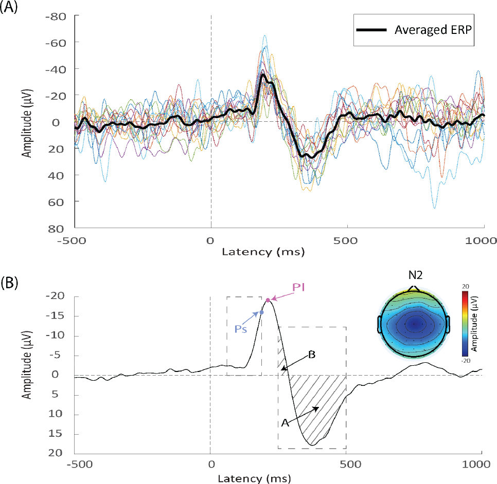
Time domain analysis. (A) Comparison between single-trial event‐related potential (ERP) waveforms (colored dotted thin lines) and the averaged ERP waveform (bold black line). Single-trial ERP waveform contains lots of noise, but simple averaging makes random noise cancel each other out and the ERP responses stands out accordingly. (B) ERP waveform and topography. Ps is the point standing for the simple peak amplitude within the dashed box, whereas Pl represents the local peak amplitude. The mean amplitude of P2 is, by definition, (A−B)/(window length), whereas A/(window length) is the mean signed amplitude. The topography of N2 amplitude is showed in the northeast subplot.

The aforementioned logic of across‐trial averaging is simple and straightforward, yet there are many intricate issues after the averaging operation. To quantify the parameters in ERPs, we typically measure the amplitude and/or latency of an ERP component for each participant and each condition or group. To measure them appropriately, however, is a big challenge for researchers.

3.1.1 Measuring amplitudes

There are at least two ways of measuring the amplitude of an ERP component. The first one is to measure the voltage at the maximum point of a waveform within a specific time window, which can be called the “peak amplitude method” [5, 7]. The other is to calculate the mean voltage of all points in a defined time window, which can be termed the “mean amplitude method” [5].

The peak amplitude method is the oldest quantification of amplitudes and is used frequently [8 –10]. However, the amplitude measured by this method is sometimes counter‐intuitive, especially when the process is implemented automatically. Fig. 2(B) illustrates clearly why the most negative point within a time window, Ps, may not be properly used to define the negative peak. Normally, we would call Pl as the negative peak instead of Ps. As Luck pointed out, we can define Pl as the “local peak”, that is, the largest point in a measurement window with upward‐going and downward‐going deflections at its left and right side [5]. In contrast, absolute maximum or minimum points can be defined as the “simple peak”.

Generally, we want to measure the local peak amplitude, but not the simple peak amplitude. It is, therefore, important that we do not confuse one with the other. Mathematically, if the maximum (or minimum) point is not at the edges of a given time window, the simple peak amplitude is identical to the local peak amplitude. In practice, we can plot the ERP waveform to identify whether the maximum point occurs at the edges. If not, there is no need to distinguish them at all, and the traditional maximum algorithm produces the local peak amplitude.

The local peak method, however, is not without its own problems [5]. First and foremost, the local peak amplitude is positively biased by the noise level. That is, the measure is generally larger than the true peak amplitude when there are noises; the larger the noise, the larger the discrepancy. Unfortunately, EEG data are noisy, even all the preprocessing procedures have been performed. The noise level partly relies on the number of trials and participants, as well as the health conditions of participants. As a result, comparing the local peak amplitudes between markedly different conditions or groups can be problematic. Second, the local peak amplitude is attenuated by the latency jitter. If the latency varies across trials or participants, which is often the case, the average local peak amplitude would be smaller than the single‐trial amplitude [as illustrated in Fig. 2(A)]. This problem renders amplitude comparisons invalid when there are significant differences in latency variability and the number of trials between conditions or groups. Third, the local peak amplitude in the average ERP waveform is not a faithful representation of the average of local peak amplitude at the single‐participant level, unless different peak latencies are aligned to the same time point [11]. Without peak latency alignment, the average waveform may not reach its peak at the same time as the single-participant waveforms do; thus, the peak amplitude obtained from the average waveform is smaller than the average of single‐participant amplitudes in most cases.

By contrast, the mean amplitude is not (at least not easily) subject to any of the three problems. However, the mean amplitude method also has its own issues. The biggest drawback is that the time window, if too wide, may contain responses of other peaks or components, and thus the resulting mean amplitude is inaccurate. Fig. 2(B) illustrates a possible scenario where the mean P2 peak amplitude (area A) is partially canceled out by the N2 response (area B). One variant of the mean amplitude, termed the “mean signed area amplitude” [5], can circumvent the problem. To computing the signed area amplitude, we simply sum together either all the positive or negative points relative to the baseline within the time window. Since only positive or negative values are summed, the problem of cancelation disappears. In the figure, the mean signed area amplitude for the P2 component would be A/L instead of (A – B)/L (the mean amplitude), where L is the length of window. The price, however, is that the sign area amplitude tends to be positively biased, which is similar to the local peak amplitude [5]. In short, none of these methods is perfect, and we need to think carefully when choosing the appropriate method to extract ERP amplitudes.

3.1.2 Measuring latencies

Latency is the time interval between the starting time point of the targeted event (e.g., stimulus onset) and a specific ERP component. There is also more than one way of measuring latency. We can simply measure the time point where the waveform reaches its peak, or estimate the midpoint of a component by locating the time point which divides the area within the corresponding time window into two halves. The former latency is called the “peak latency”, while the latter is called the “50% area latency” [5].

These two measures of latency are based on the corresponding measures of amplitude, and thus inherit the strengths and weaknesses of the amplitude measures (see above). One thing to notice is that the peak latency is more sensitive to noises than the 50% area latency. The consequence is that the peak latency shows a larger variance, leading to lower statistical power. However, the 50% area latency is sensitive to the definition of the time window for extracting the ERP component, which would result in the inaccuracy of the measurement of ERP latency.

3.1.3 Practical issues

(1) How many trials do we need?

To derive a reliable ERP waveform, we need a sufficient number of trials [3, 5]. But how can we define “sufficient”? Unfortunately, we do not have any magic number for this question. The effect size, SNR, type of analysis, as well as many other factors determine the minimal number of trials needed to obtain a reliable and robust ERP waveform [5, 12 –14]. For a large ERP component, tens of trials would be enough; for a small ERP component, we may need hundreds of trials. One thing to remember is that the SNR improves in proportion to the square root of the trial number [5]. That is, to double the SNR, we should quadruple the number of trials. Therefore, if we already have hundreds of trials, it would be unnecessary to increase the number to a thousand. Instead, we should attempt to lower the noise level by other means.

(2) Do the baseline data reflect “pure” spontaneous activity?

No. To minimize voltage offsets and drifts due to skin hydration, skin potentials, and static charges in the electrodes, we correct the poststimulus data by subtracting the baseline mean from them, immediately after epoching the data [5]. However, the prestimulus baseline may be contaminated by the ERPs from the preceding trial or participant’s anticipations of the onset of the stimulus. Since the baseline‐corrected data are the difference between the uncorrected data and the baseline mean, the poststimulus responses are influenced by the baseline activity. We, therefore, should look at the baseline activity to ensure that the effect of interest is not an artifact caused by unwanted group or condition differences in the baseline. In practice, any differences that begin in the baseline or within 100 ms of stimulus onset may be spurious [5].

(3) What reference electrode should we choose?

The reference electrode has a huge impact on the ERP waveform. But there is no universally agreed‐upon reference electrode that fits well with all research questions. Cz, Fz, linkedears, linked‐mastoids, the ipsilateral‐ear, the contralateral‐ear, the tip of the nose, the average of all electrodes, and a point at infinite have been reported in the literature as the reference [15 –17]. In general, we should avoid the reference sites that are heavily biased toward one hemisphere, near the electrode of interest, or extremely noisy [5]. A practically‐accepted option is to choose the conventional one used in the relevant research field, thus allowing for comparisons of the results with those in previous studies.

(4) How can we visualize the results?

In the time domain, we have information about electric potentials across time and electrodes. We thus can depict graphs showing how electrical potentials vary across time points (i.e., ERP waveform) and how electrical potentials vary across electrodes (i.e., ERP topography). Providing these two kinds of graphs are mandatory for ERP studies [7].

ERP waveforms display the temporal characteristics of voltage without spatial characteristics [see the waveform in Fig. 2(B)]. Oftentimes we only choose one electrode of interest or compute the average waveform of several surrounding electrodes. We can, of course, draw the ERP waveform for every electrode and put them in the same graph (e.g., butterfly plots), but that might not be helpful as the reader may not be able to see the details like the difference of ERP waveforms between different conditions or groups. An oft‐used graph derived from ERP waveforms is the differential waveform, which could be created by subtracting one ERP waveform from another, showing how the difference changes over time.

ERP topographies, on the other hand, depict how the potentials are distributed across the scalp electrodes [see the topography in Fig. 2(B)]. We need to control another variable in this sort of graph, that is, time. The time point chosen usually corresponds to the latency of the component we are interested in. Alternatively, we can calculate the mean potentials within a time window and plot the corresponding scalp topography. One rule to remember is that the time variable (e.g., the interval for computing the average) must be identical for all the electrodes [7]; otherwise, the generated scalp topography would be confusing and difficult to interpret. However, there is no restriction on how many topographies we can draw so long as every one of them follows the rule. If necessary, we could provide a series of topographies for several time points (or several time intervals) for the ERP waveform.

3.2 Time‐frequency analysis

ERP waveforms are the neurophysiological response that is both time‐locked and phase-locked to the stimulus onset. However, there are some important event‐related brain responses that are time‐locked, but not phase‐locked to the stimulus onset. To derive these brain responses, we need to perform the time‐frequency analysis, which characterizes the spectral perturbations of the data over time. Please note that Fourier transform, which is often used to extract the spectral features of resting‐state EEG [1], would not be applicable in the task‐EEG data processing, since Fourier transform ignores the temporal information and hinges on the unrealistic assumption of stationary, that is, the frequency features of the signal are assumed to be invariant over time [Fig. 3(A)].

Fig. 3.

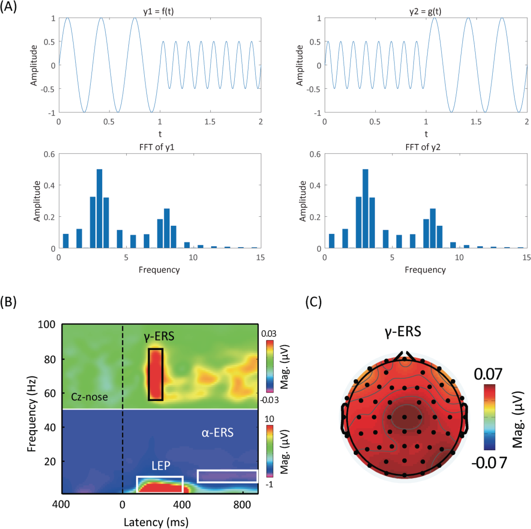
Time‐frequency analysis. (A) Shortcomings of the Fourier transform. Signals y1 and y2 are constructed from two exactly same sine waves with different temporal order. Whereas temporal characteristics of y1 and y2 are different, their results from the fast Fourier transform (FFT) are identical. (B) Time‐frequency representation. Laser‐evoked potentials (LEP), α band event‐related desynchronization (α‐ERD), and γ band event‐related synchronization (γ‐ERS) are indicated by boxes. Note that two color scales are used. (C) Topography for γ‐ERS magnitudes.

To overcome this disadvantage, we need to perform the time‐frequency analysis. Commonly used time‐frequency methods include the short‐time Fourier transform (STFT), wavelet transform, and Hilbert transform. Practically, they produce highly similar results and can be considered fundamentally equivalent [18, 19]. Therefore, we only focus on the short‐time Fourier transform in the next section, a method more intuitive and intelligible.

3.2.1 Basic ideas of the STFT

The intuition of the STFT is straightforward. It cuts a single trial into numerous brief overlaping segments (i.e., time windows) where the assumption of stationarity supposedly holds. The STFT extracts the spectrum in every time window using the Fourier transform and assign the spectrum to the midpoint in the entire window, thereby providing temporal information. The STFT thus successfully addresses — or assumes away — the problems of unrealistic stationarity assumption and the lack of temporal information of the Fourier transform.

Mathematically, the STFT for a discrete signal x(n) (n = 1, 2,…, N) is defined as

X (k, n) = \sum_{m = 0}^{N - 1} x (m) w (m - n) e^{\frac{- i 2 π k m}{N}}

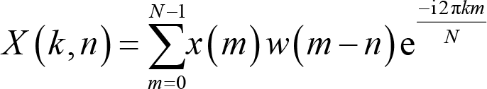
where k and n are the frequency and time localizations respectively, w is the window function, and i is the imaginary unit [20]. In practice, we can follow the six steps below to run the STFT [21]:

“1. Select a window function of finite length.

2. Place the window on top of the signal at t = t ₀.

3. Segment the signal using this window.

4. Compute the spectrum of the windowed data segment.

5. Incrementally slide the window along time.

6. Go to step 3, until the window reaches the end of the signal.”

Note that what we actually select is a window function rather than a simple window to diminish edge artifacts. Typical window functions include Hann (sometimes called Hanning), Hamming, and Gaussian windows. The Hann window is preferred since it, by definition, tapers the data to zero at its both sides [13]. The process of windowing and sliding the window along time indicates a vital issue in time‐frequency analysis: The spectra of contiguous time points would be strikingly similar, meaning the time precision of time‐frequency analysis is inherently by far poorer than the time domain analysis. Surely we can improve time resolution by narrowing the time window, but by doing so, we would have to compromise the frequency resolution, a phenomenon known as the uncertainty principle in signal processing [20].

3.2.2 Power‐based measures

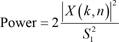
The resulting X[k, n] from the STFT is a complex series. To quantify and test the time‐frequency results statistically, we need to derive more meaningful, power‐based measures, such as magnitude, power, and power spectral density (PSD). The only difference between these measures and those used in the spectral analysis is that we have the information for both time and frequency domains in task‐related EEG, whereas the information about time is irreverent in resting‐state EEG.

Magnitude is conceptualized as the absolute value of X(k, n). However, we need to consider the fact that a window function is applied, and results from the negative frequencies are redundant for real‐valued EEG signals. Consequently, magnitude is computed as

Magnitude = 2 \frac{| X (k, n) |}{S_{1}}

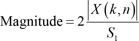
where S ₁ represents the sum of window values w_j , that is, $S_{1} = \sum_{j = 0}^{N - 1} w_{j}$ . Power is the squared magnitude and defined as

Power = 2 \frac{| X (k, n) |^{2}}{S_{1}^{2}}

PSD is a derived measure from power and calculated as

PSD = 2 \frac{| X (k, n) |^{2}}{F_{s} S_{2}}

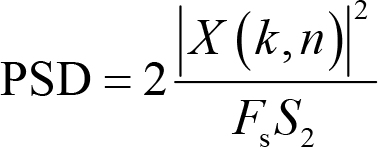
where F _s denotes the sampling frequency, and S ₂ is the sum of squared window values $\sum_{j = 0}^{N - 1} w_{j}^{2}$ . Note that the window function plays an important part in all these three formulas.

Since all three measures are, by definition, non‐negative, we solve the non‐phase locked problem in time domain analysis, which results from the cancellation of positive and negative potentials. This problem is successfully solved only if we do the STFT at the single‐trial level.

With these measures at hand, we can define two important concepts describing task‐related power changes relative to the baseline activity: event‐related synchronization (ERS) and eventrelated desynchronization (ERD). The former means the poststimulus oscillatory power is greater than the baseline power; the latter, on the other hand, means the poststimulus oscillatory power is smaller than the baseline power. The exact formulas computing them rely on the baseline correction method, a topic we discuss later in 3.2.4 Practical issues.

3.2.3 Phase‐based measures

One particularly important measure we can extract from time‐frequency results is phase, which is the angle between the real part and the imaginary part of the complex series X(k, n) resulting from the STFT. Phase angle represents the timing of certain frequency‐band activity. To test the consistency of such timing across trials, we could calculate the phase‐locking value (PLV) [22], also known as phase resetting, phase coherence, or intertrial phase clustering [13]. Formally,

PLV (t, f) = | \frac{1}{M} \sum_{m = 1}^{M} e^{i φ_{t, f, m}} |

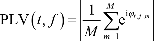
where M is the trial number, i is the imaginary unit, φ_t _, _f _,m is the phase angle on trial m at certain time‐frequency point (t, f).

PLV can also be used to quantify connectivity between electrodes. The formula calculating PLV is

PLV (t, f) = | \frac{1}{M} \sum_{m = 1}^{M} e^{i (φ_{a} - φ_{b})} |

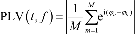
where M is the number of time points (for PLV over time) or trials (for PLV over trial), φ_a and φ_b are the phase angles from electrode a and b, respectively. Note that M can be the number of time points OR trials here, whereas it can only be the number of trials in spectral analysis. This implies that we can compute PLV over time or trial. Intuitively, PLV is the absolute value of the averaged complex polar representation of phase angle differences. PLV ranges over [0, 1] and indicates the distribution range of the phase difference series over [0, 2π). Larger PLV implies higher connectivity.

PLV suffers from the problem of a common source, meaning that spurious connectivity occurs if activities from electrodes a and b are generated by a common source. To overcome this problem, we can use the phase lag index (PLI) [23], which is defined as

PLI (t, f) = \frac{1}{M} \sum_{m = 1}^{M} sign (φ_{a} - φ_{b})

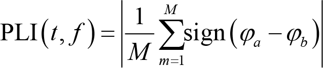
where M is also the number of time points (for PLI over time) or trials (for PLI over trial), sign() is the sign function, which equals −1 for negative inputs, 0 for zero, 1 for positive inputs. The range of PLI is also from 0 to 1, with higher values indicating higher connectivity. An improved measure, weighted PLI (wPLI) [24], is defined as

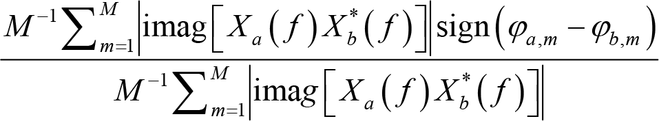
wPLI (t, f) = \frac{M^{- 1} \sum_{m = 1}^{M} | imag [X_{a} (f) X_{b}^{*} (f)] | sign (φ_{a, m} - φ_{b, m})}{M^{- 1} \sum_{m = 1}^{M} | imag [X_{a} (f) X_{b}^{*} (f)] |}

where X_a (f) is the Fourier coefficients for signals at electrode a, X_a* (f) is the complex conjugate of X_a (k), and imag() takes the imaginary part of a complex number. The complex conjugate of a complex number a + bi is a – bi. For example, 2 − 3i is the complex conjugate of 2 + 3i.

In practice, these phase‐based measures (e.g., PLV, PLI, and wPLI) were computed on the band‐passed filtered data. Note that these measures range from 0 to 1 and do not follow the normal distribution. When we compare phase‐based connectivity measures between conditions or groups, the results are bounded between −1 and 1 and are not normal-distributed, either. To facilitate meaningful statistical tests, we can Fisher‐z transform the condition or group connectivity differences to make them approximately normal‐distributed [13]. The Fisher‐z transformation is defined as

Fisher- z = \frac{1}{2} \ln (\frac{1 + C}{1 - C})

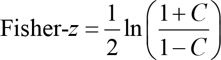
where ln() is the natural logarithm function, and C is some connectivity differences. Alternatively, we can use non‐parametric tests like the permutation test since they do not depend on the normal distribution assumption [13].

3.2.4 Practical issues

(1) How long should the time window for analysis be?

The length of the time window determines the trade‐off between time and frequency resolution. Shorter windows improve time resolution, but worsen frequency resolution; and vice versa. The window length also restricts the lowest frequency we can analyze. In theory, we can never extract the frequency information whose period is longer than the time window [13]. For example, the lowest frequency is 5 Hz if the window is 200 ms. To achieve a better SNR, we would want the window to contain two or three periods of certain frequency information, which further limits the lowest frequency we extract. In practice, we generally try out several different window lengths and choose the one that displays the best visually and statistically reasonable results [21].

(2) One STFT, one window function?

No. We can apply multiple window functions to the same data segment and average the spectrums, a method called “multitaper” [25]. In practice, to do multitaper analysis, we employ Slepian tapers, which are orthogonal to each other, rather than any arbitrarily chosen window functions [26]. The advantage of this method is that it improves the SNR, making it useful for analyzing high‐frequency activity and single‐trial data [13]. However, a higher SNR is achieved at the expense of worse time precision. The multitaper method thus is not particularly helpful for analysis that focuses on lower frequencies (e.g., below 30 Hz) or demands precise timing.

(3) How can we do baseline correction?

As in time domain analysis, baseline correction is necessary for time‐frequency analysis. One crucial reason is that raw time‐frequency power values follow the so‐called “1/f phenomenon”, meaning that the power decreases as the frequency increases [13]. This phenomenon renders it difficult to compare results from different frequency bands. Frequency‐wise baseline correction offers a partial solution.

There are four major approaches to perform the baseline correction: subtraction, percentage, decibel, and z‐score [13, 27], which are defined as follows:

Subtraction : $P o w e r_{s u b} = P o w e r - M e a n (P o w e r_{b a s e l i n e})$

Percentage : ${Power}_{per} = \frac{Power - Mean ({Power}_{baseline})}{{Mean(Power}_{baseline})}$

Decibel : ${Power}_{dB} = 10 \log_{10} \frac{Power}{{Mean(Power}_{baseline})}$

z - score : ${Power}_{z} = \frac{{Power}_{poststimulus} - Mean ({Power}_{baseline})}{SD ({Power}_{baseline})}$

where Mean(Power_baseline) is the average baseline power and SD(Power_baseline ) is the standard deviation of baseline power. It is noteworthy that the baseline need not be the entire prestimulus period. In fact, we had better choose a narrower baseline. The algorithm of the STFT implies that the power at the stimulus onset reflects the EEG activity of a time window whose midpoint is the stimulus onset. As a result, to avoid any contamination from the poststimulus activity, we should choose a baseline such that the distance between its ending and the stimulus onset is not larger than one‐half of the time window [27]. For example, if the window length is 200 ms, the baseline needs to end before −100 ms.

As for the approach per se, methods correcting the data by taking relative rather than absolute changes, that is, the percentage, decibel, and z‐score approaches, are superior to the subtraction approach in mitigating the 1/f phenomenon, making post‐corrected data more comparable between frequencies [27]. However, they all introduce a positive bias in estimating ERS and a negative bias in estimating ERD, and the resulting data are unproportionally influenced by the baseline power; the subtraction approach is free from these two problems [28]. A further advantage of the subtraction approach is that the order of baseline correction relative to averaging at the single‐participant level does not matter so long as the STFT is done at the single‐trial level. That is to say, performing the baseline correction either before or after averaging across participants provides exactly identical results. For the other three approaches, the order matters a lot. The bias in estimating ERS and ERD might be larger when relative‐changebased correction is performed at the single‐trial level than at the participant or group level [28].

(4) Should we compute connectivity measures over time or trial?

As we mentioned before, phase‐based measures, such as PLV, PLI, and wPLI, can be computed in two ways: over time or over trial. We are then forced to choose one of them. These two ways both have their own advantages and limitations [13]. Connectivity over time is less sensitive to trial‐to‐trial jitter of event timing and phase angle differences between trials. However, the epoch should be long enough for this kind of connectivity. Consequently, connectivity over time is more appropriate if we focus on high‐frequency connectivity. On the other hand, connectivity over trial puts no constraint on epoch length and achieves a higher level of evidence. Moreover, since connectivity is computed for every time point, the temporal precision is by far higher for connectivity over trial. Indeed, the STFT is not well suited for computing this connectivity; other methods like wavelet transform and Hilbert transform are preferred. The limitation is that connectivity over trial is highly sensitive to the event timing. Therefore, any uncertainty of timing may invalidate this measure.

(5) How can we visualize the results?

Time‐frequency analysis performed on a single trial produces three‐dimensional results: time, frequency, and certain measure (e.g., magnitude). A simple two‐dimensional plot thus is not adequate for visualization. To overcome this challenge, we could color the plot to add an extra dimension representing the measure we have computed [Fig. 3(B)]. Coloring the time‐frequency plot, however, is not easy. Please note that power follows the 1/f phenomenon. When using a single‐color scale, high‐frequency results would be distorted visually. That is, highly significant differences at high‐frequency bands would appear negligible compared with the results at lower frequency bands [21]. To tackle this nontrivial issue, we can use two color scales instead: one color for low frequency (delta, theta, alpha, and beta) results, the other for high frequency (gamma) results. However, we must keep in mind that the use of two color scales is for the purpose of visualization only, and that presented data must remain as they are.

In addition, we need to average the data across trials or participants. Although time-frequency results are available for every electrode, we may not want to show the results from all electrodes. Instead, we could choose one representative electrode or average several surrounding electrodes to plot time‐frequency results. To provide spatial information, we can draw a scalp topography by averaging power within the time‐frequency region of interest for each electrode [Fig. 3(C)].

3.3 Advanced techniques

Powerful as they are, time domain and time-frequency analysis are some routine analysis for task‐related EEG processing. To extract more information from the raw data, we need more advanced techniques like source analysis and single‐trial analysis.

3.3.1 Source analysis

One key feature of EEG data is that their spatial resolution is inherently poor. EEG data provide only the topographic distribution of electric potentials, not the spatial distribution of neural sources. Source analysis could be used to infer the latter from the former, which is a problem known as the inverse problem [29]. The inverse problem is notoriously difficult to solve. In actuality, this problem has no unique solution, meaning that more than one configuration of neural activity can produce the same topographic distribution and that we are theoretically unable to identify which configuration is absolutely correct for an EEG dataset. Localization of brain generators for specific electrical potentials is thus a challenging, if not impossible, task. Nevertheless, if conducted and interpreted carefully, source analysis provides valuable information about the brain regions generating the EEG activities recorded at the scalp, which is very helpful in a lot of basic and clinical applications. In practice, there are many methods to estimate the source, which are implemented in several freely- available softwares, for example, FieldTrip, sLORETA, and RECOR [29].

3.3.2 Single‐trial analysis

Traditionally, we average all single trials to boost the SNR and extract more accurate and consist brain features. However, the operation of averaging depends on an implicit and unrealistic assumption: The single‐trial response is largely invariant across trials [30]. We have mentioned in 3.1.1 Measuring amplitudes that latency jitter often occurs and, when they are extraordinarily larger, may invalidate the local peak amplitude. Nonetheless, trial variability includes at least some physiologically relevant information [31]. Therefore, across‐trial averaging is not desirable sometimes. Single‐trial measures do not confront these problems, yet its SNR is rarely satisfactory. Single‐trial analysis attempts to enhance the SNR and accurately estimates measures at the single‐trial level. There are several categories of single‐trial analysis methods, which include temporal filtering, spatial filtering, time‐frequency filtering, and model‐fitting approaches [30]. When properly conducted, single‐trial analysis enables us to extract plentiful dynamic information, such as single‐trial latency, amplitude, and morphology. This dynamic information allows us to reveal some additional information by performing a within‐subject correlation [32] and provide useful features for machine learning [33].

4 Concluding remarks and caveats

EEG is an old but powerful technique for revealing the neural implementation of human psychology. In this paper, we have introduced some of the basic and advanced EEG signal processing methods for task‐related EEG. Important temporal (ERP amplitude and latency)

and spectral measures (PSD, PLV, PLI, and wPLI) can be extracted to answer specific research questions (Fig. 1). For those who want to learn EEG signal processing more comprehensively and deeply, we highly recommend three book‐length materials: (1) An Introduction to the Event‐Related Potential Technique [5]; (2) EEG Signal Processing and Feature Extraction [34]; (3) Analyzing Neural Time Series Data: Theory and Practice [13]. Another helpful source is the YouTube channel by Cohen (https://www.youtube. com/channel/UCUR_LsXk7IYyueSnXcNextQ), which offers practical video lecturelets for analyzing EEG data free of charge.

Powerful as it is, we should not abuse EEG technique. Importantly, the proper use of EEG requires us to pay attention to the following critical issues.

4.1 Always good data first

The importance of rigorous experimental design and good data can never be overstated. Fancy data analysis will not save a poorly designed study. This is why we reiterate this point here again, even though we have discussed it in 2.1 Good data first. To acquire good data, we should think carefully about our hypothesis and design experiments accordingly before starting to collect data officially. Pilot studies are beneficial and oftentimes necessary since we cannot think of and avoid all problems prior to conducting the study in person. Rigorous study design guarantees good data in principle. In reality, EEG data are always noisy and need meticulous preprocessing to actually get the promised good data.

4.2 Always checking assumptions

All mathematical models have their own assumptions and are only effective when the assumptions are satisfied. It is, therefore, always mandatory to check them. For example, the Fourier transform relies on the assumption of stationarity. When the signal is nonstationary, spectral analysis with the Fourier transform can lead to misleading results. We can check assumptions mathematically or visually. The former is surely stricter and more precise; the latter, however, is more intuitive. If the model is robust against violation of some assumptions, a visual inspection can be extremely useful. We thus encourage more frequent use of visualization in assumption checks.

4.3 Taking advantage of the common knowledge

There is currently no universally accepted standard for EEG analysis. Recommendations from researchers in different fields may vary tremendously, and it is hard to determine which one is the correct one. “Correctness” of the recommendation may even be ill‐defined since the criteria for perfect analysis are themselves controversial and, in some cases, inconsistent. The solution is to respect the common knowledge in the field. For example, if most researchers reference the data to the nose tip, we can safely do the same thing. At least, our results are comparable to those already published, and any divergence can be explained more easily without involving methodological inconsistency.

4.4 Basic analysis before advanced ones

In the present article, we have mainly introduced the basic analysis and briefly mentioned the more advanced ones. This practice is, of course, partly due to the abstruseness of advanced analysis, but it should also remind us that the basics are more important. Findings from advanced analysis are suspicious, though not definitely false, if not supported by basic results, for example, ERP or time‐frequency results. For non‐methodological studies, we believe that the focus should be on the basic analysis and the resulting measures, unless there are a priori reasons to do otherwise.

4.5 Describing analysis in the methods section

As a general requirement, we should describe our analysis in detail in the “Methods” section. For example, we should pro″vide: the type of electrode, interelectrode impedance, the locations of the recording electrodes, the reference electrode, the sampling rate, filtering parameters, artifact identification and rejection procedures, the length of baseline, the baseline correction method, ERP amplitude and latency determination methods, the type and length of the window in time‐frequency analysis, and the like [7, 13].

With these caveats in mind, we can exploit the power of EEG technique appropriately to gain valuable insights into how the brain supports and implements human psychology.

Supplemental Material

Supplemental Material, 10.26599_BSA.2020.9050018 - Demystifying signal processing techniques to extract task-related EEG responses for psychologists

Supplemental Material, 10.26599_BSA.2020.9050018 for Demystifying signal processing techniques to extract task-related EEG responses for psychologists by Libo Zhang, Zhenjiang Li, Fengrui Zhang, Ruolei Gu, Weiwei Peng and Li Hu in Brain Science Advances

Supplemental Material

Supplemental Material, BSA20200018_suplemental_1Matlab_scripts - Demystifying signal processing techniques to extract task-related EEG responses for psychologists

Supplemental Material, BSA20200018_suplemental_1Matlab_scripts for Demystifying signal processing techniques to extract task-related EEG responses for psychologists by Libo Zhang, Zhenjiang Li, Fengrui Zhang, Ruolei Gu, Weiwei Peng and Li Hu in Brain Science Advances

Supplemental Material

Supplemental Material, BSA20200018_Suplemental_2sub_stft - Demystifying signal processing techniques to extract task-related EEG responses for psychologists

Supplemental Material, BSA20200018_Suplemental_2sub_stft for Demystifying signal processing techniques to extract task-related EEG responses for psychologists by Libo Zhang, Zhenjiang Li, Fengrui Zhang, Ruolei Gu, Weiwei Peng and Li Hu in Brain Science Advances

Footnotes

Conflict of interests

The authors have declared that no competing interests exist.

Acknowledgments

This work was supported by the National Natural Science Foundation of China (No. 31822025, No. 31671141). The funders had no role in study design, data collection and analysis, decision to publish, or preparation of the manuscript.

References

Zhang

, et al. Demystifying signal processing techniques to extract resting-state EEG features for psychologists. Brain Sci Adv. 2020, 6(3):189–209

Peng

. EEG preprocessing and denoising. In EEG Signal Processing and Feature Extraction Hu

Zhang

Eds. Singapore: Springer Singapore, 2019.

. ERP experimental design. In EEG Signal Processing and Feature Extraction Hu

Zhang

, Eds. Singapore: Springer Singapore, 2019.

Hempel

. Philosophy of Natural Science. 1st ed. Upper Saddle River, USA: Prentice Hall, 1966.

Luck

. An Introduction to the Event-Related Potential Technique. 2nd ed. Cambridge, USA: The MIT Press, 2014.

. Electroencephalography, evoked potentials, and event-related potentials. In EEG Signal Processing and Feature Extraction Hu

Zhang

, Eds. Singapore: Springer Singapore, 2019.

Picton

Bentin

Berg

, et al. Guidelines for using human event-related potentials to study cognition: recording standards and publication criteria. Psychophysiology. 2000, 37(2): 127–152.

Iannetti

. Neural indicators of perceptual variability of pain across species. Proc Natl Acad Sci USA. 2019, 116(5): 1782–1791.

Thompson

Zhang

, et al. Music reduces pain unpleasantness: evidence from an EEG study. J Pain Res. 2019, 12: 3331–3342.

10.

Peng

Tang

Zhang

, et al. Neurobiological mechanisms of TENS-induced analgesia. Neuroimage. 2019, 195: 396–408.

11.

Cai

Xiao

, et al. Human brain responses to concomitant stimulation of Aδ and C nociceptors. J Neurosci. 2014, 34(34): 11439–11451.

12.

Boudewyn

Luck

Farrens

, et al.

How many trials does it take to get a significant ERP effect?

It depends. Psychophysiology. 2018, 55(6): e13049.

13.

Cohen

. Analyzing Neural Time Series Data. Cambridge, USA: The MIT Press, 2014.

14.

Huffmeijer

Bakermans-Kranenburg

Alink

, et al. Reliability of event-related potentials: the influence of number of trials and electrodes. Physiol Behav. 2014, 130: 13–22.

15.

Teplan

. Fundamentals of EEG measurement. Meas Sci Rev. 2002, 2(2): 1–11.

16.

Yao

. A method to standardize a reference of scalp EEG recordings to a point at infinity. Physiol Meas. 2001, 22(4): 693–711.

17.

Yao

Wang

Oostenveld

, et al. A comparative study of different references for EEG spectral mapping: the issue of the neutral reference and the use of the infinity reference. Physiol Meas. 2005, 26(3): 173–184.

18.

Bruns

Fourier-, Hilbertand wavelet-based signal analysis: are they really different approaches?

J Neurosci Methods. 2004, 137(2): 321–332.

19.

Le van Quyen

Foucher

Lachaux

, et al. Comparison of Hilbert transform and wavelet methods for the analysis of neuronal synchrony. J Neurosci Methods. 2001, 111(2): 83–98.

20.

Freeman

Quiroga

. Imaging Brain Function with EEG. New York, USA: Springer New York, 2013.

21.

Zhang

. Spectral and time-frequency analysis. In EEG Signal Processing and Feature Extraction Hu

Zhang

, Eds. Singapore: Springer Singapore, 2019.

22.

Lachaux

Rodriguez

Martinerie

, et al. Measuring phase synchrony in brain signals. Hum Brain Mapp. 1999, 8(4): 194–208.

23.

Stam

Nolte

Daffertshofer

. Phase lag index: assessment of functional connectivity from multi channel EEG and MEG with diminished bias from common sources. Hum Brain Mapp. 2007, 28(11): 1178–1193.

24.

Vinck

Oostenveld

van Wingerden

, et al. An improved index of phase-synchronization for electrophysiological data in the presence of volume-conduction, noise and sample-size bias. Neuroimage. 2011, 55(4): 1548–1565.

25.

Mitra

Pesaran

. Analysis of dynamic brain imaging data. Biophys J. 1999, 76(2): 691–708.

26.

Slepian

Prolate spheroidal wave functions, Fourier analysis, and uncertainty-V: the discrete case. Bell Syst Tech J. 1978, 57(5): 1371–1430.

27.

Roach

Mathalon

. Event-related EEG time-frequency analysis: an overview of measures and an analysis of early gamma band phase locking in schizophrenia. Schizophr Bull. 2008, 34(5): 907–926.

28.

Xiao

Zhang

, et al. Single-trial time-frequency analysis of electrocortical signals: baseline correction and beyond. Neuroimage. 2014, 84: 876–887.

29.

Lei

. Source analysis. In EEG Signal Processing and Feature Extraction Hu

Zhang

, Eds. Singapore: Springer Singapore, 2019.

30.

. Single-trial analysis. In EEG Signal Processing and Feature Extraction. Hu

Zhang

, Eds. Singapore: Springer Singapore, 2019.

31.

Spencer

. Averaging, detection and classification of single-trial ERPs. In Event-related Potentials: A Methods Handbook Handy

, Ed. , USA: The MIT Press, 2005.

32.

Iannett

Hughe

, et al.

Determinants of laser-evoked EEG responses: pain perception or stimulus saliency?

J Neurophysiol. 2008, 100(2): 815–828.

33.

Huang

Xiao

Hung

, et al. A novel approach to predict subjective pain perception from single-trial laser-evoked potentials. Neuroimage. 2013, 81: 283–293.

34.

Zhang

. EEG Signal Processing and Feature Extraction. Singapore: Springer Singapore, 2019.