Genome-wide studies of time of day in the brain: Design and analysis

Abstract

Transcriptome profiling at different times of day is powerful for studying circadian regulation in model organisms and humans. To date, 24 h profiles from many tissue types suggest that about half of all genes are circadian-expressed somewhere in the body. However, few of these studies focused on the brain. Thus, despite known links between circadian disruption and neurological disease, we have virtually no mechanistic understanding. In the coming decade, we expect more genome-wide studies of time of day in different brain diseases, regions, and cell types. We expect just as many different approaches to the design and analysis of these studies. This review considers key principles of circadian tran scriptomics, with the goal of maximizing utility and reproducibility of future studies in the nervous system.

1 Introduction

To adapt to the earth’s day-night cycle, animals evolved circadian (~24 h) clocks that control the timing of biochemical, physiological, and behavioral functions [1, 2]. From flies to humans, a “central clock” in the brain synchronizes with the environment and transmits time of day cues to local clocks throughout the body [3, 4]. In mammals, the central clock is a network in a specialized region of the hypothalamus, called the suprachiasmatic nucleus (SCN) [5 –7].

At the cellular level, the clock is a feedback loop involving core transcriptional activators and repressors that generates a ~24 h molecular oscillation. This mechanism and its components are remarkably conserved throughout evolution. Starting with Konopka and Benzer’s discovery of the genetic basis of circadian behavior [8], the fly and mammalian clock research communities established a core circadian mechanism conserved over 600 million years of evolution (Fig. 1 and Table S1). For example, Clock was the first mammalian clock gene identified [9 –11]. Only later was it found to also serve a core function in the Drosophila clock (clk) [12]. Conversely, core repressors in mouse (Per1/2) [13, 14] were identified by homology to the known repressor per from Drosophila [15 –18].

Fig. 1.

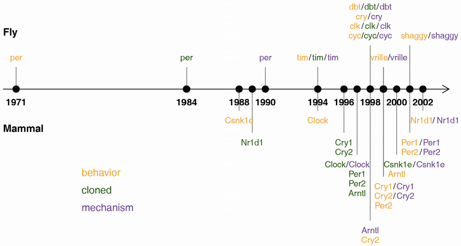
A history of clock gene discovery in flies and mammals. Gene color shows the stages of discovery as core clock genes (details in Table S1). For example, Nr1d1 was originally cloned (green) as non-clock genes in mammals, but only later found to be important in the clock mechanism (purple) and circadian behavior (orange).

With core clock genes and mechanisms elucidated by the early 2000s, a big question remained: how do molecular clocks drive physiology? Applying technology available for genome-wide mRNA profiling, chronobiologists began characterizing large numbers of clock-regulated “output” genes in flies and mice [19 –23]. These efforts now extend to many model organisms, and recently to humans.

2 CNS transcriptome: enter time-of-day

The number of circadian transcriptome studies has increased steadily over the past 20 years [24]. However, the number of circadian–brain studies has not. Circadian gene expression profiles exist for only 5 of the ~70 functionally distinct areas (https://mouse.brain-map.org/static/atlas) in the mouse brain––SCN [21, 23, 25, 26], pituitary [27], hypothalamus, brain stem, and cerebellum [28]. None of these studies has evaluated the impact of disease state.

Approximately 100 circadian-expressed genes were identified in each of the mouse hypothalamus, brain stem, and cerebellum (Fig. 2) [28]. This is far fewer than the number of rhythmic genes detected in other peripheral tissues (e.g., over 2000 circadian-expressed genes in the liver), which may be due to cellular heterogeneity in the brain. Future profiling of neuronal, or glial, subpopulations [29, 30] will help answer this question. While the core clock genes were common to all three brain regions, over 50% of the cycling genes in each region do not cycle in the other two regions. This describes a well-established feature of circadian biology––clock output is highly tissue-specific [21, 22]. To understand how clocks in the brain shape physiology, we need better spatial resolution.

Fig. 2.

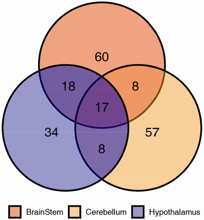
Tissue specificity in circadian gene expression across brain regions. Data taken from Zhang R. and Lahens N. et al. [28] with 2 h sampling resolution over two circadian days. Time-series data were analyzed by MetaCycle and circadian genes were defined by FDR < 0.05, rAMP > 0.1.

In the last 10 years, RNA-seq has reshaped transcriptomics. For example, several groups characterized spatiotemporal and cell type-specific transcriptome features across different regions of the mammalian brain [31]. Compared to microarrays, RNA-seq has several advantages. First, it is possible to detect transcripts in species without a reference genome sequence. Second, provided you sequence at the appropriate read depth, RNA-seq has a larger dynamic range of expression over which transcripts can be detected [32]. However, RNA-seq introduces special challenges when applied to circadian studies. This review discusses key issues that arise when designing and analyzing genome-scale time-series experiments.

3 Design and analysis of circadian transcriptome studies

A researcher faces many choices in any circadian transcriptome study. These include sampling strategy, sequencing depth, detection algorithm, and functional analysis (Fig. 3).

Fig. 3.

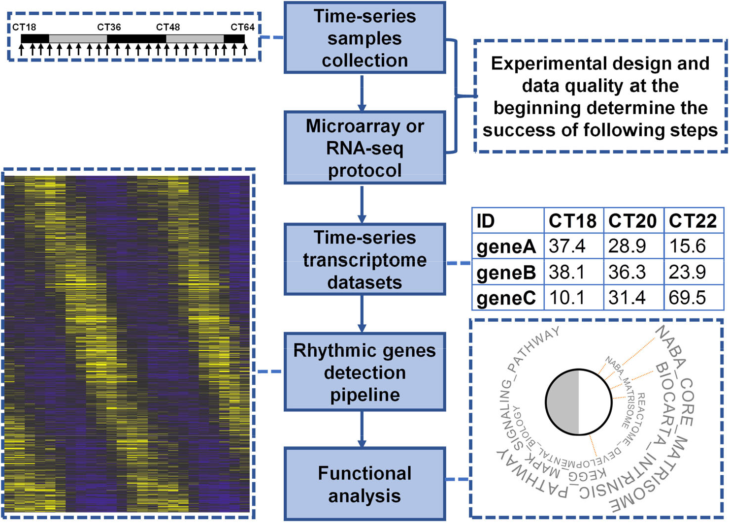
General steps of a circadian transcriptome study. The success of each study is determined by the experimental design and quality of data collected at the beginning.

3.1 Design

3.1.1 Sampling strategy

Sampling density is a key decision in any time-series experiment [24, 33]. Density is determined by the sampling resolution (e.g., every 2 h) and window (e.g., 2 days), both of which markedly impact the ability to detect rhythmic features. For example, by sampling mouse livers every 1 h for 2 days (48 samples), Hughes et al. [33] detected rhythms in more than 5000 genes (FDR < 0.05; Fig. 4, gold points). However, if we subset this same dataset to every 4 h for 2 days (12 samples), the number of rhythmic genes drops to just 17 (Fig. 4, blue points). Higher sampling resolution, therefore, can dramatically reduce the false negative (and positive) rates. Sampling resolution also impacts the ability to accurately estimate rhythmic parameters like peak phase and amplitude. For example, if we are only sampling every 6 h, it is difficult to accurately estimate the phase with an error of less than 6 h.

Fig. 4.

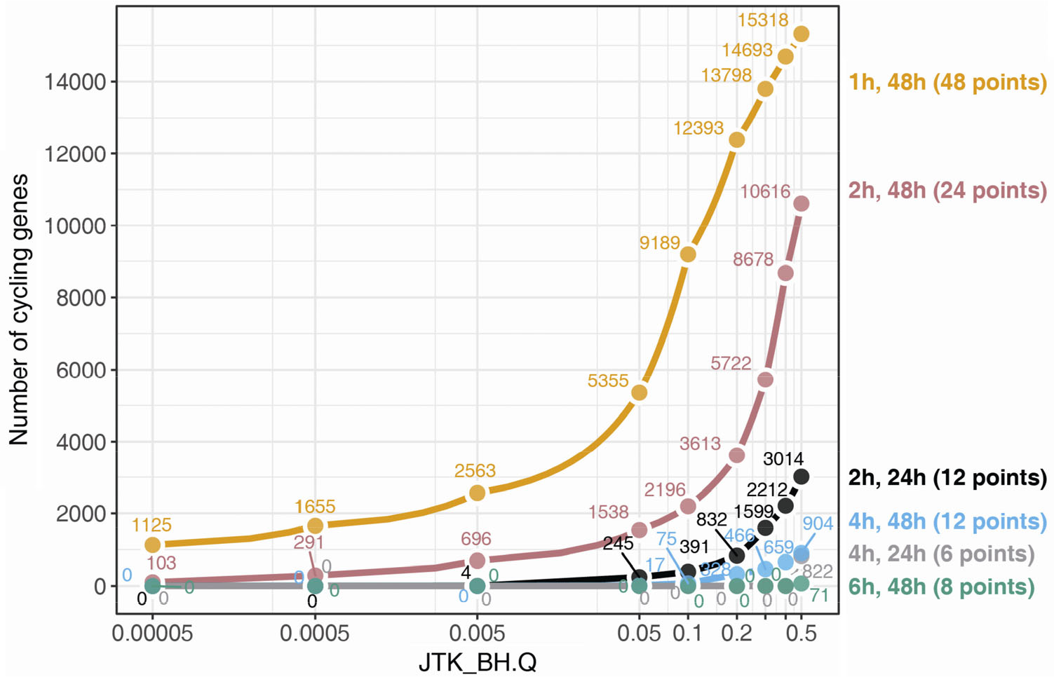
Number of circadian genes detected is strongly influenced by sampling strategy. The gold line indicates the number of circadian genes reported by JTK_CYCLE at series of BH.Q values from the gold standard time-series data collection every 1 h over two circadian days (data taken from Hughes M. et al. [33]). Other sampling strategies were simulated by down-sampling the gold standard data. The pink, blue and green lines represent data collection every 2 h, 4 h and 6 h over two circadian days, respectively. The black and grey lines indicate data collection every 2 h and 4 h over one circadian day, respectively.

A bona fide circadian rhythm persists in the absence of environmental rhythms. Experiments intended to isolate the purely circadian component are therefore run under constant conditions (e.g., 24 h darkness). Here, it is important to delay the first sampling point until ~midway into the first subjective night (e.g., CT18) to eliminate influences from the light–dark cycle itself. In addition, we recommend a sampling window that covers two complete cycles (e.g., 48 h) of the constant condition to reduce bias from outlier signals. Conceptually, one can only be confident calling a particular feature circadian if its rhythmic pattern repeats in the second cycle.

Of course, the cost of an experiment increases with sampling density. 1 h resolution is six times more expensive than 6 h resolution. This may seem prohibitive for 1 h sampling, but higher resolution improves accuracy and reproducibility. Put another way, the information loss in lower resolution studies is also costly. How can we strike the right balance? Benchmarking experiments [33, 34] suggest that 2 h–2 days density (e.g., sampling every 2 h for two circadian cycles) is a “sweet spot” for information gain. Of course, collecting and processing 24 samples is not always realistic. A lower sampling density may suffice when testing new and/or expensive technology or working with difficult to collect samples [35]. For example, when working with tiny brain regions, challenges include isolation of target cell/region, extracting adequate RNA, and verifying sample purity. A lower sampling resolution is reasonable for this kind of study. Ultimately, the most important factor for any experiment is that the results are reproducible. A study that misidentifies hundreds to thousands of “clock-regulated” transcripts slows research.

3.1.2 Sequencing depth

For RNA-seq, cDNA fragments are sequenced to obtain short sequencing reads from one end (single-end sequencing) or both ends (pair-end sequencing). Unlike microarrays, in an RNA-seq experiment, the percentage of expressed transcripts that are detected is determined by the sequencing depth. To detect a rare transcript or variant, or if studying a complex transcriptome from a larger genome, deeper sequencing is required. Sequencing depth also impacts the power of a time-series study [36], where the aim is to characterize dynamic patterns of expression over time. This requires many more reads (per gene) than what is required to simply determine whether a gene is expressed or not. For example, at 0.6 million reads per sample, we detect the expression of the Drosophila clock gene tim, but cannot discern a rhythm (Fig. 5). Only at ≥ 5M reads per sample for Drosophila can we confidently conclude that tim is rhythmically expressed.

Fig. 5.

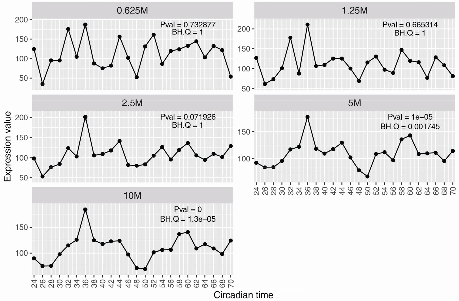
Sequencing depth impacts the temporal profile of the Drosophila timeless (tim) gene. Fly heads were collected every 2 h over two circadian days (data taken from Li J et al. [83]). The sequencing depth reached 10M for all samples. From this dataset, a down-sampling strategy was used to generate time-series datasets with sequencing depth as 5M, 2.5M, 1.25M and 0.625M for each sample. The statistical values were from MetaCycle analysis of each dataset.

In general, the power to detect rhythmic profiles scales with sequencing depth. For example, by applying a threshold of FDR < 0.05, twice as many circadian genes were detected in Drosophila heads at 10 million reads per sample compared to 1.25 million reads (Fig. 6). Thus, unlike microarray experiments, the detection power of time-series RNA-seq depends on sequencing depth. What’s the appropriate depth for a particular study? In simulations, at least 10–15 million (flies) and 50 million (mammals) paired-end reads per sample are required to detect most highly-expressed rhythmic genes [36].

Fig. 6.

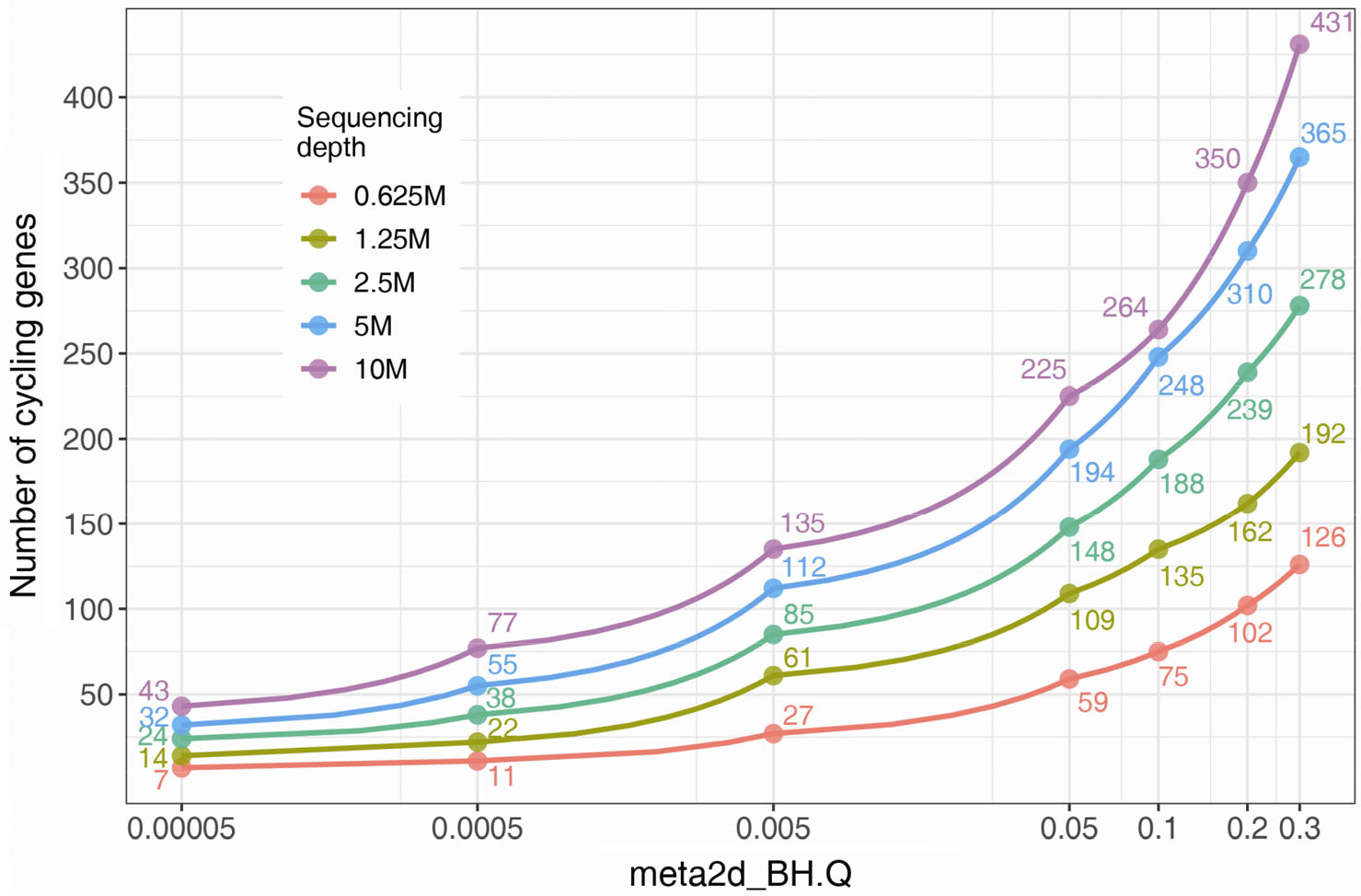
Number of detected cycling genes in Drosophila head is influenced by the sequencing depth. Same data as Fig. 5. The number of MetaCycle reported circadian genes at series of BH.Q cut-offs were indicated with red, yellow-green, green, blue and purple for datasets with sequencing depth at 0.625M, 1.25M, 2.5M, 5M and 10M reads per sample.

3.1.3 Cost and research objective

Although general rules are handy, the sampling and sequencing choices for a circadian study should ultimately align with the research aim. For example, 2 h–2 days density with 50M reads per sample is necessary if the goal is a comprehensive identification of all rhythmically-expressed genes and accurate phase estimation in mouse. On the other hand, a lower sampling density may be enough if the goal is to assess whether a functional clock exists in a tissue. And, although RNA-seq is “state of the art”, microarrays remain a good option if the goal is to profile known genes.

Of course any study design is restricted by the research budget. The cost of designing a high-quality circadian transcriptome experiment may exceed the budget. Before any study, we suggest performing a thorough survey of available public datasets. CircaDB [37], CircadiOmics [38], CGDB [39] and CirGRDB [40] house dozens of circadian associated databases. In some cases, it may be possible to leverage data from experiments that have already been performed. For example, the mouse liver circadian transcriptome data was applied to study the liver circadian proteomics and metabolites [34, 41].

3.2 Analysis

3.2.1 The “golden rules”

A large group of circadian researchers recently published a consensus “golden rules” for genome-scale circadian analyses [24]. First, never duplicate and concatenate data before statistical inference, including type Ⅰ and Ⅱ manipulation (Fig. 7). Second, control for multiple hypothesis testing (detailed discussion to follow). Third, deposit raw data in public repositories, such as NCBI’s Gene Expression Omnibus or Sequence Read Archive, EMBL-EBI Expression Atlas, DDBJ Sequence Read Archive, or Genome Sequence Archive of China National Genomics Data Center.

Fig. 7.

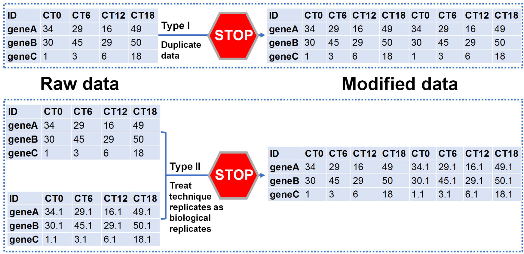
Never duplicate and concatenate data prior to statistical inference.

3.2.2 Rhythm detection

The first step is the quality control of the raw microarray or RNA-seq files. For example, the R package arrayQualityMetrics [42] detects outlier samples for Affymetrix arrays, and FastQC (https://www.bioinformatics.babraham.ac.uk/projects/fastqc/) and RSeQC [43] have been used in the quality control step of analyzing RNA-seq data. Quality samples are then pre-processed. For microarray time-series experiments, algorithms for background correction, signal calculation, and normalization are well established [44]. However, for RNA-seq, there is no current standard for read alignment, expression quantification, or normalization applied to time-series studies. Reasonable options include STAR [45] for read alignment and HTSeq [46], RSEM [47] and Kallisto [48] for mapping and quantification of RNA-seq data. Future comparisons of widely accepted RNA-seq analysis pipelines on circadian transcriptome should help to clarify best practices.

There are many computational methods available for detecting rhythms. A decade ago, Doherty et al. summarized 16 different algorithms [49]. Since then, many more were developed, including JTK_CYCLE [50], ARSER [51], LSPR [52], RAIN [53], SW1PerS [54], eJTK [55], BooteJTK [56], ABSR [57], BIO_CYCLE [58], ZeitZeiger [59], MetaCycle [60] and ECHO [61]. Which algorithm should I use? Third-party comparisons are few [62, 63], but each algorithm has pros and cons that relate to study design and objective. Specifically, the researcher should consider their (1) sampling density, (2) tolerance for false positives, (3) tolerance for false negatives, (4) interest in detecting a range of different rhythmic waveforms, and (5) preference for ease of use.

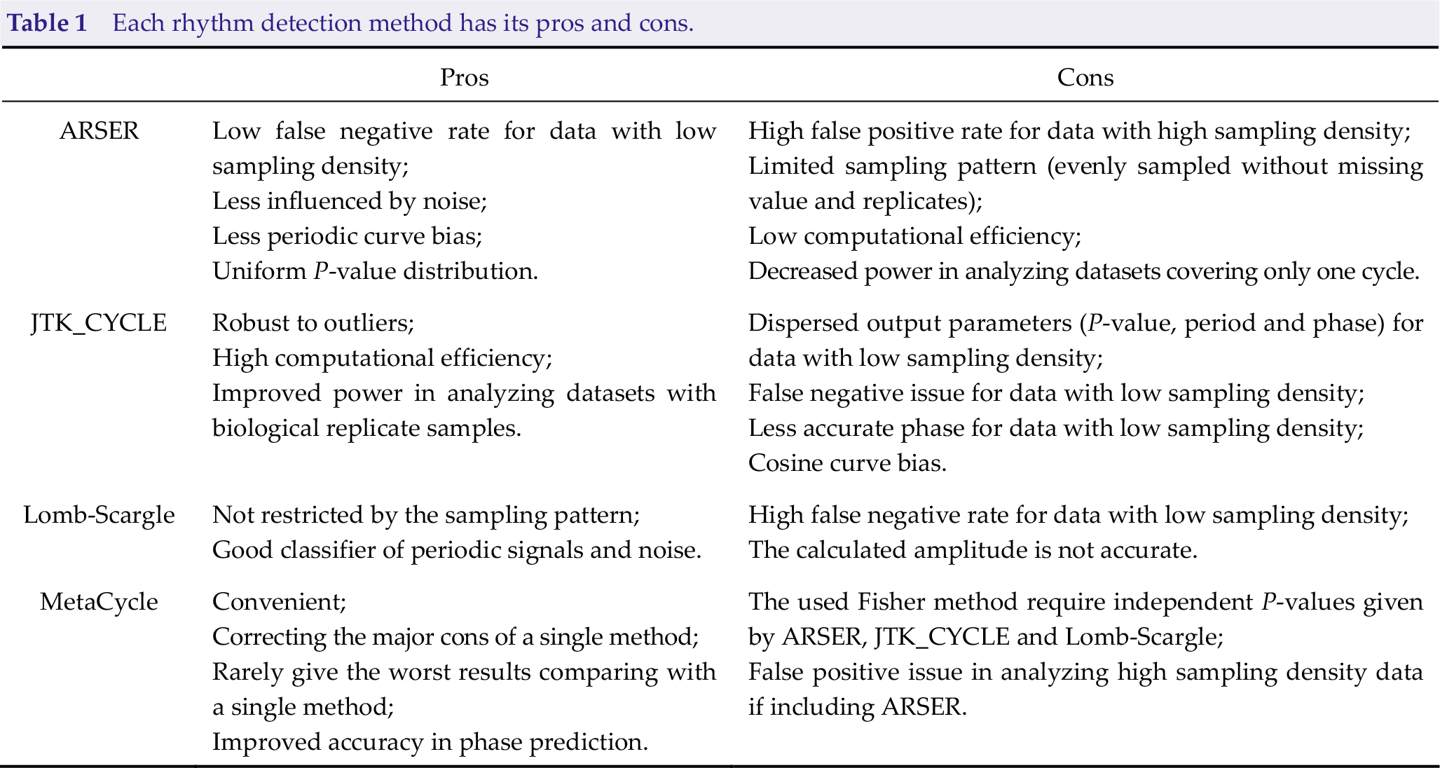
For example, three separate algorithms were incorporated into the MetaCycle package. As summarized in Table 1, ARSER has a low false-negative rate for datasets with low sampling density but presents a serious false-positive problem for datasets with high sampling density. Lomb-Scargle [64], on the other hand, has the advantage that it can handle different sampling patterns, including unevenly sampled data. But, it suffers from a high false-negative rate for data with a low sampling density. Table 1 illustrates the pros and cons of each method. The logic behind MetaCycle is an N-version programming (NVP) [65] method to explore periodic data, which is borrowed from the aeronautics industry. By taking advantage of multiple independent algorithms and a voting scheme to integrate their results, a method that performs poorly in a particular condition will be outvoted by other methods that better accommodate that condition. However, there are other outstanding detection methods not covered by MetaCycle, including RAIN [53] and BooteJTK [56]. In recent years, there have been improvements to usability (e.g., DiscoRhythm [66], and Nitecap https://nitecap.org/), differential rhythmic analysis (e.g., DODR, LimoRhyde, and CircaCompare) [67 –69], and generalizability to other “omics” data (e.g., ECHO) [61]. When applying these rhythmic detection algorithms, setting period length as 24 h is suggested for identifying circadian genes, considering (1) it is hard to accurately calculate the period length (e.g., 22 h vs. 24 h) with time-series data covering only two cycles; (2) this will improve the statistical power and computational efficiency without multiple testing series of period length values.

Table 1.

Each rhythm detection method has its pros and cons.

	Pros	Cons
ARSER	Low false negative rate for data with low sampling density; Less influenced by noise; Less periodic curve bias; Uniform P-value distribution.	High false positive rate for data with high sampling density; Limited sampling pattern (evenly sampled without missing value and replicates); Low computational efficiency; Decreased power in analyzing datasets covering only one cycle.
JTK_CYCLE	Robust to outliers; High computational efficiency; Improved power in analyzing datasets with biological replicate samples.	Dispersed output parameters (P-value, period and phase) for data with low sampling density; False negative issue for data with low sampling density; Less accurate phase for data with low sampling density; Cosine curve bias.
Lomb-Scargle	Not restricted by the sampling pattern; Good classifier of periodic signals and noise.	High false negative rate for data with low sampling density; The calculated amplitude is not accurate.
MetaCycle	Convenient; Correcting the major cons of a single method; Rarely give the worst results comparing with a single method; Improved accuracy in phase prediction.	The used Fisher method require independent P-values given by ARSER, JTK_CYCLE and Lomb-Scargle; False positive issue in analyzing high sampling density data if including ARSER.

There is an unmet need for comprehensive and objective comparisons between methodologies. Qualitative evaluation requires quality bench-marking datasets––both simulated and real. Recent contributions of CircaInSilico [24] and Simphony [70] offer tools to simulate the impact of sampling patterns, outliers, and noise. Yet unsolved issues remain. For example, current tools simulated independent rhythmic profiles, but new tools are needed to address the co-regulation feature of rhythmic genes. Apart from simulation, we need more experimentally validated circadian datasets from different tissues [71].

As a final note, we suggest great caution around claims of “more sensitive detection”, as finding more rhythmic features is not necessarily better. False positives waste resources in validation experiments and can lead (and have led) to erroneous conclusions.

3.2.3 Cutoffs

After the detection algorithm is run, researchers classify transcripts as rhythmic or not. Often this is a simple “yes” or “no”, decided by a statistical test value. There are potential problems with this way of thinking. We outline them, starting with the most easily fixed.

1. Measures of statistical confidence MUST be corrected for multiple hypothesis testing. P-values are usually calculated independently for each transcript. For a given transcript, then, we may interpret p = 0.01 as meaning “there is only a 1 percent chance that the rhythm we detect is due to chance”. However, a transcriptome study involves thousands of these independent tests. If we choose p < 0.01 as cutoff for “yes” or “no”, then we must acknowledge that we will wrongly assign “yes” to hundreds of transcripts. Should dozens or more of tissues be analyzed, you would incorrectly conclude that the entire transcriptome is rhythmic. For this reason, the false discovery rate (FDR or BH.Q value) [72] is used to control for multiple hypotheses in genome-scale data. Nevertheless, there may be experimental designs and detection algorithms for which FDR is too restrictive. For example, if the false-negative rate is much higher than the false-positive rate (e.g., all FDR = 1), P-value may be a useful guide if combined with additional evidence.

2. Many algorithms estimate the amplitude (i.e., a measure of magnitude) of transcript oscillation over the study window. This is another frequently used cut-off. However, the amplitude calculation (maximum difference from the average expression level along time, or baseline) is strongly influenced by overall expression level, and may not reflect the strength of oscillation (Fig. 8). In the mouse liver, for example, the amplitude (AMP) of Ugt2b34 is ten-fold greater than the core clock gene Per2. From this, we might conclude that the Ugt2b34 oscillation is 10 times stronger than Per2. But, when we control for differences in baseline expression between the two genes, the conclusion changes dramatically: Per2 is 10 times stronger! In general, we suggest using relative amplitude (rAMP)––the ratio of amplitude to baseline when thresholding by rhythm magnitude [60].

Fig. 8.

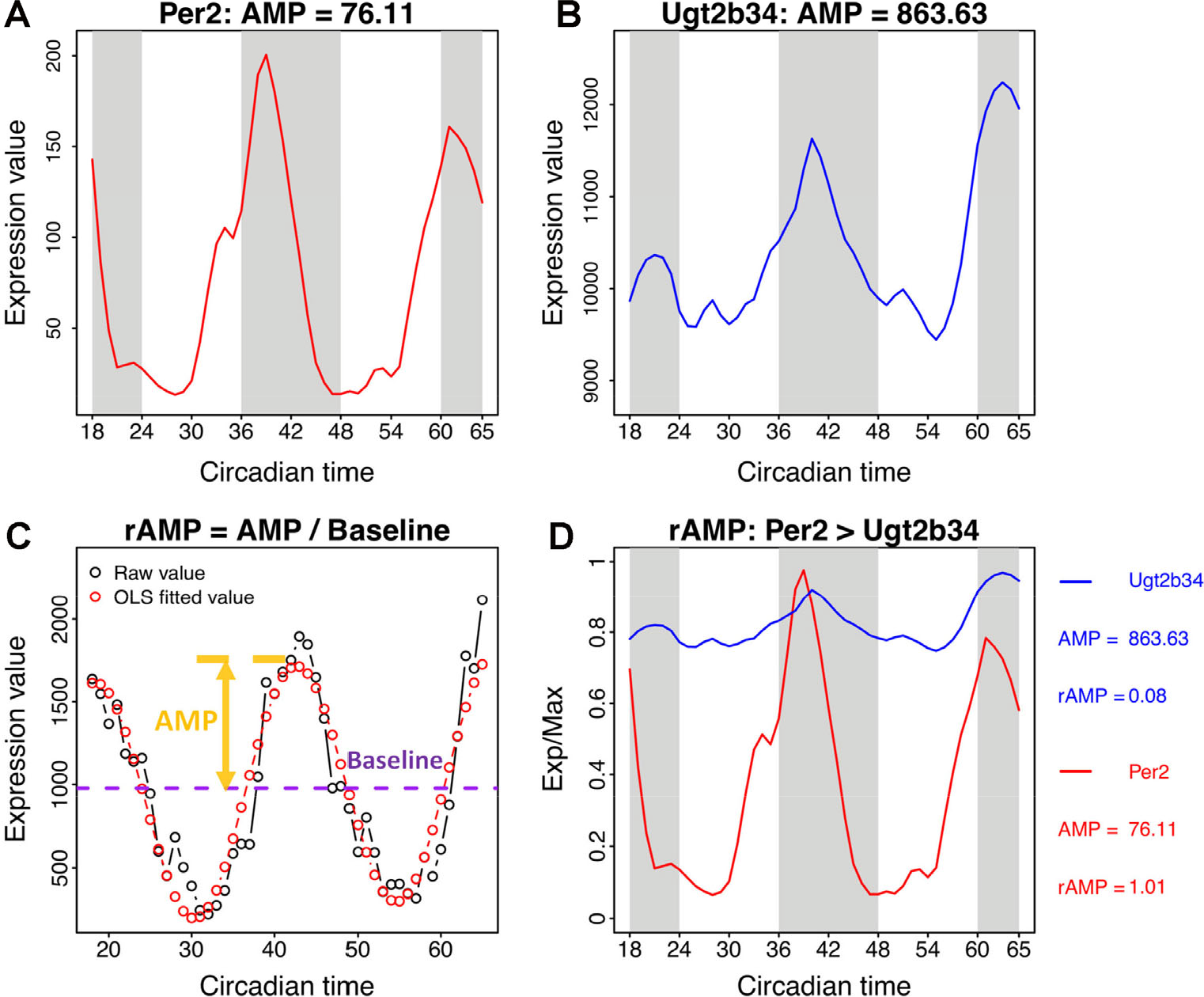
The relative amplitude value (rAMP) is a better index indicating robustness of oscillation. The expression profiles and amplitude values of Per2 and Ugt2b34 are shown in (A) and (B). (C) The rAMP is the ratio between amplitude and baseline level of the time-series profile. (D) The rAMP reflects the cycling strength of genes at different expression levels. The amplitude value is associated with the general expression level, which indicates highly expressed genes may always have larger amplitude than lowly expressed genes. The rAMP could be used to compare the amplitude values among genes with different expression levels. For example, Ugt2b34 has a larger amplitude than Per2, but its rAMP is smaller than Per2.

3. Sometimes fold change (max/min) is used to evaluate the magnitude of oscillation. Indeed, this is easily interpretable and controls for differences in expression level. However, fold-change can be strongly influenced by outlier values in the time-series data. rAMP, therefore, has the added advantage that it is less sensitive to a noisy measurement.

4. Regardless of the evaluation criterion, a discrete “yes” or “no” strays from biology. A transcript that “just made the cutoff” has more in common with the one that “just missed the cutoff” than it does with those higher on the list of “yes”. Rather than imposing rigid cutoffs, we support looking at (and presenting) data over a range of cutoffs, and thinking about the findings from a probabilistic perspective instead of a binary checkbox.

3.2.4 Validation and pathway analysis

We strongly recommend using prior knowledge to validate experimental results. For example, when profiling samples with an intact circadian clock, the core clock genes will be among the most rhythmic in the genome. In addition, the estimated phase relationships between clock genes should match with current knowledge: e.g., Arntl and Per1 should peak at roughly opposite times. For species without prior knowledge, it may be informative to evaluate the circadian gene orthologs to related species.

The biological information from a circadian transcriptome study is more important than the number of rhythmic features. Pathway analyses (DAVID, EnrichR, GSEA or PSEA) [73 –76] can shed light on how specific biological functions are coordinated in time. For example, a circadian transcriptome study in the SCN found cycling genes enriched for synaptic vesicle trafficking machinery [21] that was later implicated in SCN clock function [77].

4 Circadian transcriptomics on human brain samples

This review focused on time-series in animal models, but most of the principles also apply to circadian transcriptomics on the human brain. Disrupted circadian rhythms are associated with neurodegenerative and neuropsychiatric disease [78], but the underlying mechanisms are virtually unknown. Three recent studies analyzed gene expression in different brain areas as a function of sampling time (i.e., time of death). Hundreds of rhythmic transcripts were identified in different human brain regions, including prefrontal cortex, anterior cingulate cortex, hippocampus, amygdala, nucleus accumbens, and cerebellum [79 –81]. Importantly, circadian profiles for many of these transcripts were dramatically altered in the presence of brain disease and/or aging. At present, circadian biology is not a clinical consideration for the prevention, diagnosis, or treatment of neurological disease. There is accumulating evidence, however, that the molecular clock plays an important role in maintaining homeostasis in the brain.

5 Conclusion

We recognize that circadian studies of the brain will be critical to understand the molecular nature of CNS disease and pathology. However, for these studies to be maximally informative, including informing potential therapeutic avenues, they need to be designed, conducted and analyzed properly. Here we have reiterated best practices and guidelines necessary for conducting these studies in a rigorous and informative fashion. These best practices consider: model organism, sampling strategy, sequencing depth, rhythmic signal detection and statistical cutoffs. We list well-accepted “golden rules”, though not hard and fast rules, to deal with these issues. Successfully completing these studies will provide insight into CNS disorders that are influenced by the clock, such as major depressive disorder, bipolar disorder, and neurodegenerative disorders (e.g., Parkinson’s disease, Alzheimer’s and Huntington’s disease) [78, 82]. In doing so, genome-wide study of time of day in the brain will offer new avenues to treat these CNS disorders.