Dual-Contrast Cellular Magnetic Resonance Imaging

Abstract

Negative contrast magnetic resonance imaging (MRI) methods using magnetic susceptibility shifting agents have become one of the most important approaches in cellular imaging research. However, visualizing and tracking labeled cells on the basis of negative contrast is often met with limited specificity and sensitivity. Here we report on a MRI method for cellular imaging that generates a new contrast with a distinct topology for identifying labeled cells that has the potential to significantly improve both the sensitivity and the specificity. Specifically, we show that low flip-angle steady-state free precession MRI can be used to generate fast three-dimensional images of tissue that can be rapidly processed to generate quantitative metrics enabling color overlays indicative of regions containing labeled cells. The technique substantially improves the ability of MRI for detecting labeled cells by overcoming the fundamental limits that currently plague negative contrast methods.

THE REALIZATION that any media tagged with local magnetic susceptibility (LMS) altering agents can produce signal voids in an image has paved the way for visualizing and tracking biologic agents (cells, genes, peptides, etc.) with magnetic resonance imaging (MRI).^1–5 LMS variations can lead to destructive interference of signals emitted by spins (protons) resident in affected imaging voxels. This results in the regions surrounding LMS-shifting media to appear hypointense (dark) relative to unaffected regions in magnetic resonance (MR) images. Typically, these dark zones are discriminated as image artifacts in MR images. ⁶ However, given that dark regions can also be mimicked by regional heterogeneity in spin density or differences in the relaxation properties with a given tissue, more reliable MRI methods for tracking LMS-shifted agents are necessary. ⁷ Recently, a number of off-resonance positive contrast (ORPC) imaging methods that permit the visualization of cells labeled with LMS-shifting agents as hyperintense (bright) zones have been developed.^8,9 These techniques have the potential to improve MRI-based visualization of tagged biologic media by selectively imaging the off-resonant spins near regions of LMS variations. However, large bulk magnetic susceptibility shifts, such as those found between heart–lung interfaces, ¹⁰ compounded by practical limitations in field shimming, along with coil sensitivity variations, limit the benefits offered by ORPC imaging methods.

Fast low-angle positive-contrast steady-state free precession (FLAPS) MRI ¹¹ is a potential alternative to cellular MRI methods that identify the presence of labeled cells strictly on the basis of either negative or positive contrast. It is ideally suited for cellular MRI because it has the capacity to generate both positive and negative contrasts with a distinct topology. In brief, the FLAPS technique relies on the unique spectral response of the steady-state free precession (SSFP) MRI signal to generate signal enhancement from off-resonant spins, while suppressing the signal from on-resonant spins at relatively low flip angles (Figure 1). In addition to the positive contrast generated by the weakly off-resonant spins, the spins in and around the core of the LMS-shifting media (such as labeled cells) experience large deviations from the central frequency, leading to intravoxel dephasing that is observed as negative contrast in FLAPS images. ¹²

In this work, we demonstrate the ability of FLAPS MRI to identify the presence of labeled cells with both positive and negative (hence the term dual) contrast within a single image through in vitro, ex vivo, and in vivo studies. Our findings show that the dual-contrast nature of the FLAPS approach offers significant advantages to the field of cellular MRI.

Figure 1.

Dependence of transverse component of steady-state free precession (SSFP) signal intensity relative to signal available at thermal equilibrium as a function of the deviation from center frequency in units of 1/TR, where TR is the time between the radiofrequency pulses. At low flip-angle (FA) (< 30°), the signal intensity of the on-resonant spins (spins resonating at center frequency) is significantly lower than that of the off-resonant spins (those that are resonating at frequencies that deviate from the center frequency). Given that the signal intensity difference between off- and on-resonant spins is positive, a relative hyperenhancement can be observed around local magnetic susceptibility (LMS) media, such as superparamagnetic iron oxide–labeled cells at low FA. As the FA is increased, the signal enhancement surrounding the LMS media is decreased. Given that large frequency variations are found at the center of the susceptibility-shifting media, intravoxel dephasing results in dark zones, permitting the visualization of the magnetic perturbers to be observed as a dark core surrounded by a bright ring.

Methods

Cell Preparation and Labeling

A rat 3230 adenocarcinoma (R3230Ac) cell line, derived from a spontaneous mammary carcinoma of the Fischer 344 rat, was used throughout the study. The cells were cultured in Dulbecco's Modified Eagle's Medium (DMEM, Invitrogen, NY) with 10% fetal bovine serum (Biosource, UT) and streptomycin at 37°C in air with 5% CO₂ atmosphere in a 75 cm² culture flask. Media were replaced every 3 to 4 days. Subsequently, the cells were incubated overnight in the culture medium for 24 hours with superparamagnetic iron oxides (SPIOs) (Feridex I.V., Advanced Magnetics, Cambridge, MA) with iron concentration of 20 μg/mL in each group. Unincorporated iron particles were removed by repeated washing with phosphate-buffered saline (PBS). Samples of the labeled cells were set aside for evaluation of cell labeling efficiency (n = 6) and to quantify uptake of iron particle by cells (n = 3). Multiple samples were used to assess the reproducibility of the experiments. From the remaining cells, six sets of sample preparations (one set for each experiment) were made. A total of 7.5 × 10⁶ labeled cells were used per experiment.

Histologic Analysis and Quantification of Iron Uptake

Histology was used to validate the cellular uptake of SPIOs. The labeled cells, set aside for the labeling efficiency studies, were transferred to six-well plates and sterilized cover slips (diameter 15 mm) were placed over the samples. A similar number of unlabeled samples were prepared in an identical manner. The samples were stored at 37°C. Approximately 5 hours after, the labeled cells adhered to the cover slips and were fixed for 10 minutes with 10% formalin. The fixed cells were washed three times with PBS, stained by Prussian blue, incubated with a 1-to-1 mixture of 6% HCl (Sigma-Aldrich, St. Louis, MO) and 2% potassium ferrocyanide (Sigma-Aldrich) for another 30 minutes. Next, the cells were washed in PBS and observed using light microscopy. Labeling efficiency was determined by manual counting of Prussian blue–stained and unstained cells using a Zeiss microscope at 40× magnification using Axiovision 4 software (Carl Zeiss, Gottingen, Germany). Cells were considered Prussian blue positive if intracytoplasmic blue or granules could be detected.

The amount of iron taken up by labeled cells was assessed with an ICP-AES spectrometer (Varian, Palo Alto, CA). After labeling, washing, and harvesting, cell pellets were dissolved in 1% sodium dodecyl sulfate. For iron content measurements, the spectrometer was set to 238.204 nm (emission wavelength for iron) and calibrated. Iron content per cell was determined by dividing iron concentration (pg Fe/mL) by cell concentration (cells/mL).

Sample Preparation and In Vitro MRI Protocol

Each labeled cell preparation was washed three times with PBS, harvested through trypsinization, suspended in culture media, and further subdivided into four groups (4 × 10⁶, 2 × 10⁶, 1 × 10⁶, 0.5 × 10⁶). The labeled groups and one unlabeled group (4 × 10⁶) of cells were transferred into separate 1.5 mL Eppendorf test tubes and centrifuged at 1,000 rpm for 5 minutes to form cell pellets. Each sample was placed in a warm water bath (approximately 37°C) and scanned individually.

MRI studies were performed using a whole-body 3.0 T Tim Trio system (Siemens Healthcare, Erlangen, Germany) equipped with maximum gradient amplitudes and slew rates of 40 mT/m and 200 mT/m/ms, respectively. Integrated system body coils were used for radiofrequency excitation, and eight-channel head coils were used for signal reception. Following scout scans to find the optimal imaging plane containing the cells, balanced SSFP and gradient-recalled echo (GRE) sequences were prescribed. SSFP scans were prescribed with the following imaging parameters: field of view (FOV) 156 × 156 mm²; slice thickness 1.5 mm; matrix size 192 × 192; TE/TR 2.4/4.8 ms; pixel bandwidth (BW) 965 Hz; FA 5°, 15°, 30°, 45°, and 90°; number of signal averages 5; and acquisition time (TA) 4.6 seconds. Twenty-five SSFP scans (five cell preparations at five different FAs) were acquired. GRE sequences were prescribed with the following scan parameters: FOV and slice thickness were the same as SSFP scans; matrix size 128 × 128; TE/TR 10/100 ms; BW 260 Hz; FA 25°; number of signal averages 1; and TA 13 seconds.

Ex Vivo Preparation and Cell Imaging Protocol

Four SPIO-labeled cell preparations (1 million cells per preparation made identical to those used in the in vitro studies) were injected into excised sections of fresh skeletal muscle tissue (chicken breast). Each cell preparation was injected at three different locations within a given tissue specimen. This procedure was repeated for each tissue specimen. Each muscle sample containing the labeled cells was immersed in a standard saline bath and imaged. Three-dimensional FLAPS and GRE imaging were performed on each ex vivo preparation. Scan parameters for three-dimensional FLAPS imaging were as follows: FOV 81.25 × 200 mm²; slice thickness/slab thickness 0.4/100 mm; interpolation factor 2; spatial resolution (interpolated) 0.4 × 0.4 × 0.4 mm³; BW 930 Hz; TE/TR 2.4/4.8 ms; FA 5°; number of signal averages 4; and TA 255 s. The optimum FA for the FLAPS acquisition was based on previous studies in skeletal muscle. ¹² The scan parameters for the three-dimensional GRE scans were the same, except for the following: TE/TR 10/100 ms; FA 25°; BW 255 Hz; number of signal averages 1; and TA 1,331 s.

Animal Preparation and In Vivo MRI Protocol

Two Wistar rats were studied using the protocol and procedures approved by our institution. Rats were anesthetized with ketamine (80 mg/kg) and xylazine (3 mg/kg) and acepromazine (2 mg/kg) via intraperitoneal (IP) injection. Once sedated, labeled (1 × 10⁶) and unlabeled (1 × 10⁶) cells (prepared in an identical fashion to in vitro studies) were injected into the contralateral hindlimb muscles of the rats. The animals were inserted into a polyvinylchloride pipe to immobilize the limbs. The plastic tube containing the rat was transferred to the scanner bed. Phased array carotid coils (element size 6 × 7 cm²) were placed over the portion of the plastic tube with the hindlimbs of the animal. The coils were secured with Medical Tape (3M, St. Paul, MN). All imaging studies were performed on the 3 T system used for in vitro studies. GRE sequences were prescribed with the following scan parameters: FOV 56.25 × 100 mm²; slice thickness/slab thickness 0.8/12.8 mm; matrix size 72 × 128; in-plane resolution 0.4 × 0.4 mm²; TE/TR 40/2000 ms; BW 260 Hz; FA 15°; number of signal averages 1; and TA 255 s. Subsequently, three-dimensional FLAPS scans were prescribed with the same scan parameters, except for the following: matrix size 144 × 256; TE/TR 2.55/5.10 ms; BW 620 Hz; FA 5°; number of signal averages 4; and TA 82 s. Once the imaging studies were completed, rats were euthanized with an intravenous injection of Euthasol (sodium pentobarbital 150 mg/kg, IP) and by a bilateral thoracotomy.

Analysis of MRIs

In vitro images were analyzed with the aim of generating quantitative information, whereas ex vivo and in vivo data were used for qualitative evaluation of the image contrast that can be generated in tissue containing SPIO-labeled cells. Two complementary metrics were used to assess the contrast differences as a function of FA for each cell preparation: (1) global contrast to noise ratio (gCNR) and (2) local contrast (LC). gCNR was defined as the mean intensity difference between bright pixels and adjacent background normalized by image noise, whereas LC was computed as the mean intensity difference between bright and dark pixels normalized by the standard deviation of the intensity of the background, accounting for the number of bright, dark, and background (isointense) pixels (details below).

gCNR Measurement

To evaluate the FA dependence of gCNR, regions of interest (ROIs) were manually drawn on the SSFP images in air, the region exhibiting the positive contrast signal, and background (a region near, but outside, the signal enhancement region). The standard deviation of the signal within the ROI drawn in air (σ_air) was assumed to be representative of the image noise, whereas the mean signal value contained within the ROI drawn in the adjacent region devoid of signal enhancement was taken as the mean background signal (S_b). The signal enhancement (positive contrast signal, S_p) was extracted from the ROI containing the SPIO-enhanced region using a previously used method in the positive contrast signal characterization studies. ⁹ Using these measurements, gCNR was computed as (S_p – S_b)/σ_air. This was performed for each cell preparation (0.5 million, 1 million, 2 million, 4 million, and controlled samples) and was averaged across repeated experiments for each FA. The results are reported as mean ± standard error.

LC Measurement

To measure LC, both SSFP and GRE images were ported into Matlab (Mathworks, MA). In general, LC was computed as a product of relative area (number) of affected pixels and local contrast to noise ratios (CNRs). More specifically, to compute LC from GRE and SSFP images, the following metrics were used: for ROIs that contain both bright and dark regions, LC was defined as (N_b + N_w)/N_bgd · ((W – B)/σ_bgd), whereas for ROIs containing only a dark region (such as the GRE images), LC was defined as (N_b/N_bgd) · ((B – B_bgd)/σ_bgd), where N_b, N_w, and N_bgd are the number of bright, dark, and background pixels, respectively; and W, B, and B_bgd are the mean signal intensities computed by averaging the pixel intensities identified as bright, dark, and background, respectively. To compute LC from the in vitro studies, a rectangular ROI (36 × 36 pixels) was drawn around each feature enhancement pattern. The mean (μ) and standard deviation (σ) of all of the intensity values inside the ROI were found. Pixels with intensity below the μ – σ level were classified as dark, whereas pixels above the μ + σ were classified as bright. All other pixels were identified as background. For each class, the total number of pixels (with at least two contiguous pixels) and respective mean intensities were computed and recorded. If no bright pixels were found, the metric defaults to the second case of only dark regions present. For the GRE images, only two classes were used, dark and background.

Dual-Contrast Image Filter

Ex vivo and in vivo FLAPS images were processed using a specialized nonlinear filter designed to locate SPIO-labeled cells on the basis of their dual-contrast appearance. The filter was designed to amplify and identify the dual-contrast topology of image locations containing the three classes (bright, dark, and background) of pixel intensities. The dual-contrast image filter (DCIF) operates on a rectangular n × n sliding window of pixels (n = 7 for ex vivo and n = 31 for in vivo), and the three classes of pixels were identified as described above. For each class, the total number of pixels and their intensity average were recorded. The DCIF algorithm altered the pixels in the source images according to the relationship,

${\mathrm{Q}}_{\mathrm{D}}=\frac{27{\mathrm{N}}_{\mathrm{b}}\cdot {\mathrm{N}}_{\mathrm{w}}\cdot {\mathrm{N}}_{\text{bgd}}\cdot (\mathrm{W}-\mathrm{B})}{\left(2{\mathrm{n}}^6\cdot {\sigma }_{\text{bgd}}\right)},$

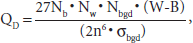
where N_b, N_w, N_bgd, W, B, and σ_bgd are as defined above. Note that 27/n⁶ (product of the pixel numbers from the different classes when the classes are uniformly distributed) and 2σ_bgd (a measure of the deviation between dark and bright pixel intensities) are normalization factors.

Statistics

One-way analysis of variance (ANOVA) with Tukey post hoc analysis was performed within each group of cell preparation to identify any statistical differences in gCNR and LC at the different FAs. The Student t-test was used to test whether there were any statistical differences in LC measured from the GRE images and FLAPS images (SSFP images at the optimal FA). Nonlinear regression analyses with Box-Lucas fit were performed between the estimated number of cells and the contrast metrics (gCNR and LC) for each FA. Fitting equation was defined as the Box-Lucas curve, y = a(1 – e^−bx), where y is the measured quantity (gCNR or LC) and x is the estimated number of labeled cells, with a and b denoting the fit parameters, where a, b > 0. Given that gCNR and LC are bounded from above (thermal equilibrium magnetization) and below (zero, dark pixels from complete destructive interference), Box-Lucas functional behavior is a representative model of the contrast behavior (ie, there is a minimum when × = 0 and an asymptotic maximum for large values of x, with the rate constant of 1/b). A linear correlation analysis was performed between the total number of bright and dark pixels from the FLAPS images against the total number of dark pixels from the GRE images for each estimated cell number. All results were deemed statistically significant for p < .01. Local contrast sensitivity (LCS), a measure of the sensitivity of the FLAPS and GRE methods for identifying the number of cells on the basis of image contrast was defined as the first derivative of the LC with respect to number of labeled cells; that is, LCS = a · b · e^−bx.

Results

Cell Labeling Efficiency

Light microscopy of the Prussian blue staining of labeled cells revealed abundant intracellular uptake of SPIOs into the cytoplasm; conversely, no stainable iron was detected in the unlabeled cells. This enhancement pattern is observable in Figure 2A. Labeling efficiency was consistently reproducible at approximately 100%. The iron content per cell determined by inductively coupled plasma atomic emission spectrometry (ICP-AES) is shown in Figure 2B. The results showed that, in comparison with the control group, the labeled-cell groups had a significantly greater mass of iron (labeled cells: 4.75 ± 0.11 pg Fe/cell, control: 0.19 ± 0.01 pg Fe/cell, p = .005).

Figure 2.

Cell labeling with superparamagnetic iron oxides (SPIOs). A shows Prussian blue stained histologic images of unlabeled (left panel) and labeled (right panel) cells with SPIOs at 40× magnification. B shows the results from ICP-AES analysis confirming the substantial differences in intracellular SPIO uptake within the cells.

Figure 3.

Representative axial in vitro images of cells scanned with steady-state free precession (SSFP) and gradient-recalled echo (GRE) imaging methods. All imaging methods showed that the image-based size of the cell pellets is directly related to the number of labeled cells. For brevity, SSFP images acquired at only 5°, 30°, and 90° are shown. At 5° (SSFP), a hyperenhancement surrounding a signal void with a reasonable level of background suppression was observed. At 90° (SSFP), the hyperenhancement was no longer visible, but the center of the cell pellet was visualized as a signal void. At 30° (SSFP), a hyperenhancement surrounding signal void is observed with sufficient background detail. GRE images depicted regions containing cells as signal voids. FA = excitation flip angle.

In Vitro Studies

Signal Features

FLAPS-based acquisitions of cells loaded with SPIOs were visualized as regions of central signal voids confined by regions of positive contrast, whereas the GRE images were visualized with signal voids in regions containing labeled cells. This is shown in Figure 3.

Contrast Dependence

FLAPS-based gCNR and LC were strongly dependent on FA, increasing from 5°, peaking at 30°, and descending to baseline levels at 90°. One-way ANOVA with Tukey post hoc analysis showed that gCNR and LC (labeled cells) are greatest when the FA is 30° (Figure 4, A and B). This was not observed among the control group. In particular, at an FA of 30°, all labeled cell preparations yielded gCNR > 10 and LC > 4. A paired t-test showed that, at every set of labeled cell number studied, the LC from FLAPS was significantly greater than that computed from GRE images (p < .001).

Curve Fits

For the FLAPS method using the optimal FA of 30°, nonlinear regression analysis between gCNR or LC against number of labeled cells showed strong correlations: gCNR (a = 50.5 ± 9.53, b = 0.42 ± 0.15, r² = .97) and LC (a = 14.3 ± 2.03, b = 0.51 ± 0.15, r² = .97), where a and b are Box-Lucas fit parameters. When the same curve-fitting procedure was applied to the GRE LC data, once again, a strong correlation was observed (r² = .92), with a = 7.40 ± 1.38 and b = 0.60 ± 0.24. Note that the curve-fitting procedure assumed the control group to be equivalent to zero number of labeled cells. The results from the curve fitting between LC and number of labeled cells for GRE and FLAPS (FA 30°) are shown in the top panel of Figure 4C (gCNR not shown for brevity). The mean LC (experiment), LC (fit), and LCS ratio of FLAPS to GRE were 1.76 ± 0.12, 1.78 ± 0.05, and 1.98 ± 0.20, respectively. LCS computation for FLAPS (FA 30°) and GRE showed that the FLAPS LCS was larger than that of GRE LCS over the range of number of labeled cells (0 < × ≤ 4 million).

Figure 4.

Results from analysis of in vitro steady-state free precession (SSFP) and gradient-recalled echo (GRE) images. A, Mean global contrast to noise ratio (gCNR) values measured from the multiple experiments showed a direct relationship between gCNR and number of labeled cells (×). The gCNR values computed at every × showed peak values at a flip angle (FA) of 30°. The gCNR values obtained at 5° and 90° are shown for reference; for brevity, the results from 15° and 45° are not shown. At these extreme FAs, the gCNR values are relatively constant and do not show a strong dependence on x. B, Mean local contrast (LC) values measured from the SSFP (FA 30° or FLAPS) and GRE experiments also showed a direct relationship between LC and x, whereas no strong dependence on LC is observed with SSFP imaging at the extreme FAs. C, Top panel: Mean LC values from FLAPS and GRE images were fit to a Box-Lucas exponential (details in text). The results showed that LC is a nonlinear function that can be modeled by a Box-Lucas exponential and that at every x, the LC from FLAPS is greater than the LC from GRE. Bottom panel: LCS computations showed that FLAPS offers a greater sensitivity to discriminate the number of labeled cells on the basis of LC compared to GRE. D, Relative area of off-resonance influence and local contrast to noise ratio (CNR) between FLAPS and GRE images is shown as a function of x. The ratio of area of off-resonance influence between FLAPS and GRE is approximately one, whereas the ratio of local CNR between FLAPS and GRE is significantly larger than one. Line of identity is shown for reference.

Bright versus Dark: Pixel Count versus Mean Cluster Intensity

Linear regression analysis between the total affected pixels in FLAPS (number of bright pixels [N_w] + number of dark pixels [N_b], FA 30°) and GRE images (N_b) obtained over respective labeled number of cells showed a strong correlation (r² = .99, p < .01) with the line of best fit given by Y₁ = 1.8 + 0.48X₁, where Y₁ = area of the total affected pixels computed from optimal FLAPS images and X₁ = area of the total number of dark pixels from GRE images; errors in intercept and slope were 5.2 and 0.03, respectively. The relative mean number of dark pixels in FLAPS images compared with the total affected pixels was 0.53 ± 0.03. The relative area of dark pixels in FLAPS images compared with the total area of dark pixels in GRE images was 0.26 ± 0.02. The mean ratio of total number of affected pixels relative to the number of background pixels (N_bgd) between optimal FLAPS ((N_w + N_b)/N_bgd) and GRE (N_b/N_bgd) over the different labeled cell clusters was 1.08 ± 0.08. The mean ratio of local CNRs between FLAPS ((W – B)/σ_bgd) and GRE (B – B_bgd) over the different labeled cell clusters was 1.58 ± 0.19, where W, B, and B_bgd are the mean signal intensities from bright, dark, and background pixels, respectively. The relative ratios between the number of pixels affected by off-resonance shifts and the local CNR as a function of number of labeled cells for FLAPS and GRE images are shown in Figure 4D.

Ex Vivo Studies

Visualization of the presence of labeled cells within the skeletal muscle using the three-dimensional GRE and FLAPS methods was possible on a consistent basis, although the contrast characteristics between the two types of acquisitions were markedly different. GRE images depicted the presence of labeled cells as hypointense zones, whereas the FLAPS images showed the same regions as smaller hypointense regions surrounded by hyperenhancement. Minimum intensity projections through the imaging volume showed substantial hypoenhancement throughout the GRE and FLAPS images, albeit the dark blooming artifacts were noticeably reduced in the FLAPS images. Maximum intensity projections through the imaging slab reduced the conspicuity of the labeled cells in the GRE images while providing nearly full hyperenhancement over the regions containing cells. When the GRE and FLAPS images were processed using DCIF, GRE images showed negligible DCIF values (Q_D), whereas the FLAPS images identified the regions containing the labeled cells with substantial DCIF values. A representative image set showing these observations from a thin slab of the three-dimensional images is shown in Figure 5. Note that in the GRE image there is significant enlargement (“blooming”) of the hypointense regions that markedly reduces the regional specificity of the cells. This effect is not observed in the FLAPS image.

In Vivo Studies

Labeled and unlabeled cells injected into the contralateral hindlimbs of the Wistar rats were visualized on GRE and FLAPS images. On the GRE images, the unlabeled and labeled cells appeared dark, albeit the labeled cells were significantly darker. On the FLAPS images, the unlabeled cells appeared as a mildly dark zone surrounded by a set of weakly bright pixels, whereas the labeled cells appeared as a substantially dark core surrounded by intense brightness. DCIF applied to the GRE image produced negligible DCIF values (Q_D), whereas same filtering of the FLAPS image generated marked DCIF values in the region of labeled cells and minimal DCIF enhancements in the region of unlabeled cells. A representative axial image set with these observations is shown in Figure 6. Note that in the GRE image, it is difficult to identify regions containing labeled cells on the basis of signal voids alone because there are several nonspecific dark zones within the image that are unrelated to the labeled cells. Also note that the regional brightness in the tissue–air interface in Figure 6C is correctly not enhanced as regions containing cells by the nonlinear filter because it does not contain a dark core. A purely ORPC imaging method would incorrectly identify the bright boundary as a region containing labeled cells.

Discussion

Tagging cells with susceptibility-shifting media has been the method of choice for visualizing cells of interest with MRI. Traditional MRI methods have relied on off-resonance approaches that depict the regions containing labeled cells as signal voids. Given that signal voids also appear within MRIs for reasons other than the presence of susceptibility-shifting agents, newer methods that enable the visualization of regions containing labeled cells as zones of hyperintensity have been developed. However, even ORPC imaging methods have pragmatic limitations.

This work demonstrated that FLAPS MRI has the capacity to identify the labeled cells with greater confidence and sensitivity. The key findings from this study were as follows: FLAPS MRI (1) provides a unique signature to identify cells labeled with LMS agents such as SPIOs; (2) offers a nearly twofold increase in sensitivity for detecting labeled cells compared with the GRE (standard) method in vitro; (3) has the capacity to generate only negative or only positive contrast images within and surrounding regions containing labeled cells through simple postprocessing methods; and (4) has the potential to improve the regional specificity of the cells compared with the standard (GRE) methods by significantly reducing the undesirable blooming artifact.

These results reveal the multifold advantages of the FLAPS approach for cellular MRI. First, a nearly twofold increase in LC and LCS with FLAPS MRI compared with GRE in vitro is an important finding because one of the principal hurdles of cellular MRI is detection sensitivity. Accentuating the sensitivity of cellular MRI via advancement in imaging technologies that empower clinical scanners for visualizing and tracking cells of interest is highly desirable. These sensitivity increases have the power to bridge the gap between basic cellular MRI studies and clinical medicine. Although the work here demonstrated that a twofold increase in detection sensitivity is possible in vitro with FLAPS MRI compared with GRE MRI, whether this sensitivity enhancement translates to in vivo imaging remains to be investigated. Second, the dual-contrast feature of labeled cells within a FLAPS MRI significantly enhances the specificity of detection. Low spin density, relaxation changes within the FOV, and blooming artifacts, all of which are well-known limitations of GRE imaging, are no longer impediments that decrease the specificity of labeled cells. Moreover, the proposed dual-contrast method also overcomes much of the limitations of positive contrast imaging methods as well. In particular, positive contrast imaging methods are vulnerable to bulk frequency shifts, typically arising from air–tissue interfaces, signal from fat protons, or coil sensitivity variations, all of which appear as hyperenhancements. Although many of the ORPC imaging methods have addressed issues related to fat, the inability of clinical scanners to provide a uniform magnetic field through shimming procedures is a central difficulty with ORPC approaches, particularly at higher clinical field strengths (eg, 3 T). These limitations are critical, for instance, while imaging regions surrounding the heart–lung interface or portions of the brain near the sinus cavity, both of which are subject to magnetic field inhomogeneities that shift the center frequency by as much as 200 Hz at 3.0 T.^10,13,14 Given that these field variations permeate from the air–tissue interfaces into ROIs, imaging LMS-shifted regions containing labeled cells requires methods that can discriminate between bulk and LMS shifts. This remains an open issue with off-resonance positive and negative contrast approaches. An attractive feature of the FLAPS-based method is that it provides a unique and easily identifiable contrast pattern that is generated from the labeled cells. This pattern then permits the use of detection algorithms and image filters, such as the one employed in this work, that distinctly identify the topologic pattern associated with the LMS-shifted cells. Moreover, ORPC imaging methods require fusing an anatomic image with a positive contrast image, a complicated image-processing task in itself. This is not necessary with FLAPS MRI because the desirable contrast and anatomic features are captured within the same image. Third, FLAPS MRI is a fast imaging method, a feature that is highly desirable, particularly in the clinical setting. Fourth, FLAPS MRI uses low FAs, compared with standard spin-echo approaches, reducing concerns related to tissue heating in acquisitions that demand ultra-high spatial resolutions, which necessitate multiple averaging. The inability to control or minimize the thermal dose delivered during cell imaging studies may compromise cell function and the overall benefits of imaging studies. Finally, and perhaps most importantly, the method can be used across all clinical scanner platforms, regardless of the scanner, because the SSFP imaging is a standard MRI method, and FLAPS MRI is a special instance of SSFP imaging.

Figure 5.

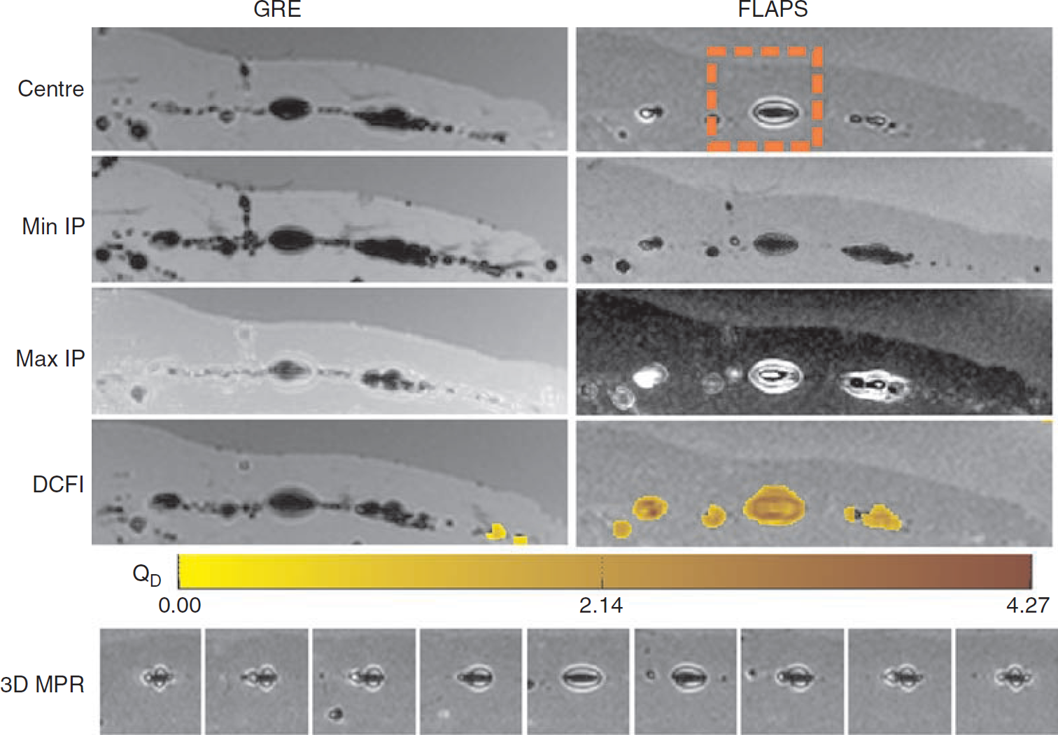
Gradient-recalled echo (GRE) and FLAPS images of labeled cells injected into ex vivo skeletal muscle. The results from the three-dimensional GRE and FLAPS acquisitions are shown along the left and right panels, respectively. Panels labeled Centre, Min IP, Max IP, and DCFI show the central slice, thin minimum and maximum intensity projections, and dual-contrast filtered image overlaid on top of the corresponding central GRE and FLAPS slices, respectively. The central slice is an imaging slice from the three-dimensional volume covering a slab thickness of 4.4 mm, with the slice thickness of 0.4 mm. Labeled cells are visualized as dark regions in GRE images, whereas FLAPS images identify them as regions of dark core surrounded bright contours. Min IP shows the dark regions surrounding labeled cells in both GRE and FLAPS images, whereas Max IP through the same slab shows the labeled cells as regions of brightness. DCFI demonstrates that dual-contrast filter allows for identification and visualization of regions containing only labeled cells in the central FLAPS image. The color bar shows the output from DCIF (Q_D). Note that effectively no significant values are generated from the DCIF applied to the central GRE image. Three-dimensional MPR is a multiplanar reformation of the highlighted region (orange box) in the central FLAPS images over the full imaging volume, providing a means for visualizing the labeled cells throughout the imaging volume.

Figure 6.

Gradient-recalled echo (GRE) and FLAPS images obtained following injection of labeled and unlabeled cells into the hindlimbs of a Wistar rat. GRE (A) and FLAPS (B) with dotted and solid arrows show the sites of unlabeled and labeled cell injections, respectively. The labeled and unlabeled cells are visualized as dark regions in the GRE image, albeit the regions containing the labeled cells appear substantially darker than the region containing the unlabeled cells. In the FLAPS image, the labeled cells are visualized as regions containing a signal void surrounded by hyperenhancement, whereas the unlabeled cells are relatively less hypointense with a weak hyperenhancement. The overlay of dual-contrast filtering over the FLAPS image is shown in C, with the region containing labeled cells identified with significant dual-contrast image filter (DCIF) enhancement compared with the minimal enhancement surrounding the unlabeled cells. The color bar shows the value of the DCIF output (Q_D).

In this study, important contrast metrics were used to assess signal changes. gCNR was used to measure only positive contrast measurements and to demonstrate the FA dependence on image contrast. In addition, a more realistic metric using the area of influence by labeled cells and local contrast to noise values were used together to evaluate the signal changes as a function of the number of labeled cells. These studies showed that because the relative area of enhancement between GRE and FLAPS images was nearly one, the main factor driving the higher LC values in FLAPS images, compared with GRE images, has its source in local CNR because the mean ratio in local CNR was approximately 60% greater with FLAPS than with GRE. Also note that contrast sensitivity metrics such as the Weber or Michelson contrast^15–17 cannot be directly used to measure the local contrast generated with FLAPS because the Weber contrast does not account for features having opposing intensities (dark or bright), whereas the Michelson contrast metric assumes that regions with opposing intensities cover the same area. The LC metric can accommodate opposing intensity features and also accounts for the size of the features by using the number of pixels in the formula. To normalize the metric and incorporate a noise measurement, the standard deviation of the background pixels was used as a denominator. The histogram-based segmentation used is reasonable because it follows the theory that labeled cells will create both bright and dark areas within FLAPS images but only dark areas in GRE images.

Although this study explored the use of FLAPS-based cellular MRI, additional improvements to the method can further strengthen its utility. First, it was observed that the magnitude of DCIF is large when the n × n sliding window contains large number of pixels for each pixel class (actually, it is maximized when pixels are distributed uniformly and each class contains n²/3 pixels). It should be noted that the value n is critical because it allows for the filter to incorporate topologic information in its estimation. A large n highlights large areas that contain all pixel classes, whereas a smaller n will do the opposite. For example, compared with ex vivo analysis, in vivo analysis used a larger n. It is believed that there is a relationship between n, the distance between the hyper- and hypointense zones, the concentration of labeled cells, and optimum FA. This remains to be investigated. Furthermore, additional topologic information such as orientation and ordering of the pixel classes may be further incorporated by adopting connective segmentation and graph theory principles to improve the image filter.^18,19 Finally, ICP-AES-based quantification of iron within labeled and unlabeled cells (control) provided the verification that the contrast observed in vitro, both in GRE and FLAPS images, originated from LMS shifts. On this basis and based on previous landmark studies,^4,20 GRE imaging was used as the gold standard against which the FLAPS imaging method was compared. Although there was a significant spatial correspondence between GRE and FLAPS images with regard to regions containing iron, a histologic correspondence between regions containing iron and regions identified with FLAPS MRI to contain iron remains to be established.

The peak contrast achieved in vitro at 30° is consistent with previous explanations that relate the optimal FA to the T₁/T₂ of the surrounding medium of the LMS agents. In particular, as shown elsewhere, ¹² there is an inverse relationship between T₁/T₂ of the surrounding medium and the optimal FA for FLAPS MRI. Consequently, the optimal FA in water (in vitro) where the T₁/T₂ is approximately 1 to 2 greater than that in skeletal muscle (ex vivo and in vivo) where the T₁/T₂ is 15 to 20.

A highly sought feature of cellular imaging is the quantification of labeled cells. Past studies have shown that it may be possible to define a relationship between the number of cells and magnetic resonance transverse relaxation time constants (apparent T₂ or T₂*). However, given that the specificity of the labeled cells is often compromised in GRE images, it is often difficult to use this as a reliable metric to quantify the number of cells. This work showed that LC is exponentially related to the number of cells. Furthermore, the dual-contrast filter, using an image metric that is analogous to LC, also provides quantitative information of regions containing labeled cells. A careful investigation of how the output of DCIF, Q_D, can be used to derive quantitative information on the concentration of labeled cells from in vivo images is a natural extension of this work.