Sage Journals: Discover world-class research

Abstract

Most studies of sleep staging in rats use both multichannels electroencephalogram (EEG) and electromyogram (EMG), so it would be convenient and meaningful in some fields if sleep staging in rats could be realized using a single EEG channel. In this study, we used a single bipolar cortical EEG electrode at the frontal–parietal location with a 0.5–30 Hz filter band and a clustering sleep-staging algorithm including seven classification parameters. The agreements between the computer and two independent raters were 96.9 ± 1.1% for Wake, 97.1 ± 1.4% for non-rapid eye movement (NREM) sleep, and 91.4 ± 2.5% for rapid eye movement (REM) sleep, and the overall agreement was 96.7 ± 0.7%. These results indicate that the accuracies of sleep staging remain high even though only a single EEG channel was used and that a system based on this scheme would be suitable for realtime and long-term studies of sleep.

Keywords

Sleep staging rat electroencephalogram (EEG)

Scoring systems of sleep–wake states are employed widely in various sleep-related studies because of their high performance and reliability. In general, all algorithms used in these systems are based on various electrophysiological properties of different vigilance states.

Nowadays, most studies of sleep staging in rats exploit the characteristics of both electroencephalogram (EEG) and electromyogram (EMG) and discriminate the various stages by comparing with thresholds.^1–4 But for a long time, the application of the visually detected thresholds from one session to all the recordings from the same animal would reduce the accuracy of sleep staging because these characteristics may change with experimental manipulations (drugs, learning, etc.);⁵ hence it is necessary to check and adjust periodically to provide reliable thresholds.³ However, such a procedure would be cumbersome and would interrupt the realtime process. Therefore, a non-threshold-based method is valuable for practice.

Some pharmacological treatments may induce dissociation between the EEG and the behaviour of the animal, so the field of applications of a system relying exclusively on EEG analysis may be restricted,⁶ and only a few studies have been solely based on the EEG features up to now.^7–9 Similarly, the field of applications of a system based on EEG and EMG would also be restricted because of the same reason and the chance that the rats would sometimes augment the EMG signal to ‘fool’ the computer into scoring sleep as wakefulness.² So each system is problem-oriented and it is important to have a clear purpose for developing a new scoring system.⁶

Systems based on the characteristics of EEG and EMG need recording cables consisting of at least four wires. However, variations in recording cable weight and flexibility can have a significant impact on sleep and activity in mice.¹⁰ Hereby, these variations may have an effect on sleep in rats. Most protocols applied would induce sleep disturbances, hence damaging the reliability of the system.⁶ Compared with EMG, however, many studies have shown that EEG of rats has distinct statistical characteristics,^11,12 EEG could be acquired with electrodes at precisely defined coordinates, and the contact between an EEG electrode and the rat's skull may be better than that between an EMG electrode and the dorsal neck muscle with time elapses. So a system involving only a single EEG channel for long-term sleep study may be more effective.

In 1994, Karasinski and collaborators implanted electrodes over the right parietal cortex and the cerebellum of a rat as a bipolar cortical EEG electrode, and realized sleep staging by calculating standard deviation, skewness, kurtosis, number of zeros crossing, number of relative maxima and minima.⁷ This method is based on cluster analysis instead of threshold and it uses only EEG recording; thus, it is suitable for the long-term study of sleep, especially in studies on circadian rhythmic mechanisms of the sleep–wake cycle.⁷ The accuracy of this study was 83.0% for rapid eye movement (REM) sleep, 96.0% for Wake and 97.1% for non-rapid eye movement (NREM) sleep. Compared with other studies,^1,5 the accuracy of REM sleep was lower. Later, Robert et al. ⁸ developed an algorithm based on artificial neural networks and thresholds for the same data, and the results were 95.31 ± 1.06% for Wake, 97.43 ± 1.66% for NREM and 92.33 ± 2.27% for REM.

In fact, using the same algorithm to analyse data acquired from different electrodes, the system will give different sleep scoring results. Obviously, using different algorithms to analyse the same data from the same electrode, the systems may also give quite different results. The algorithm adopted by Karasinski et al. ⁷ omitted the low EEG frequencies (0–3.18 Hz), thus about half of the delta (δ) wave in sleep staging was ignored.⁶ As the δ and theta (θ) waves are typical waveforms during NREM and REM sleep, respectively, and also considering their contributions in sleep staging, using other electrode locations, a wider filter band and more classification parameters may lead to a better sleep staging result.

The purpose of this study is to optimize a strategy of sleep staging in rats for the long-term study of sleep with a single EEG channel and a non-threshold-based algorithm. Based on previous studies,^7,8 two bipolar cortical EEG electrodes were tested: one was the same as that used by Karasinski et al. and the other was a frontal–parietal bipolar electrode. Two non-threshold-based algorithms were tested: one was the same as that developed by Karasinski et al. and the other was an extended version with a different band-pass filter and two more EEG parameters. In our study, the results of the four cases were compared with visual analysis results of 22 h EEG and EMG recordings of five rats by two independent raters. Based on the differences among the four cases in accuracy of sleep staging, the best one for sleep staging using a single EEG channel was found and is recommended.

Materials and methods

Animals

Five male Sprague–Dawley rats were provided by the Institute of Laboratory Animal Science of Sichuan Province, China. They were housed under controlled temperature conditions (22 ± 1°C) and maintained on a 12:12 light–dark cycle (lights on at 08:00 h). Water and food were available without restriction. Rats weighed 319.8 ± 7.7 g (mean ± SD) at the time of surgery. All procedures used in this work were approved by the Animal Care Committee of the University of Electronic Science and Technology of China.

Surgery

Sterile surgery was performed under deep anaesthesia induced by intraperitoneal pentobarbital sodium (60 mg/kg). Before surgery, the rats were given atropine (1 mg/kg) subcutaneously to decrease the secretion of the respiratory tract.

To fix body position, the rats were placed in a stereotaxic apparatus (Stoelting 516003, Illinois, USA) with a pair of blunt ear bars. Two bipolar cortical EEG electrodes made of miniature stainless-steel screws (φ 0.8 mm) were screwed up for four circles to implant in the skull of each rat at a depth of about 1.3 mm. Figure 1 shows the two bipolar electrodes and 20 s of typical EEG–EMG waves for each of the three sleep–wake stages with different bipolar electrodes. A frontal electrode was implanted 4 mm anterior to the bregma and on the midline. A right parietal electrode was implanted 3.8 mm posterior to the bregma and 2 mm lateral to the midline. Another right parietal electrode was implanted 5 mm posterior to the bregma and 1.5 mm lateral to the midline. A midline electrode above the cerebellum was implanted 11 mm posterior to the bregma (Figure 1).

Figure 1
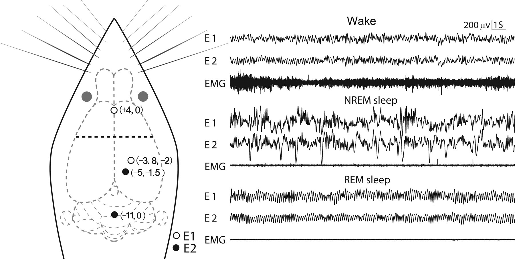
Electrode placements and 20 s of typical EEG–EMG tracings in different sleep–wake stages for different bipolar electrodes. The horizontal dashed line in bold in the rat head denotes the position of the bregma. EEG = electroencephalogram; EMG = electromyogram; REM = rapid eye movement; NREM = non-rapid eye movement

The two screws used as parietal electrodes must be burnished so as to avoid short circuit. Electrode pair E1 was the one that we proposed. It should be noted that the frontal electrode was on the sagittal suture; hence the surgery had to be performed carefully to avoid injury to the major blood vessels under the midline. Electrode pair E2 was the same as that used by Karasinski et al. To record EMG for visual classification, two Formvar-insulated (except at the part contacting with muscles) nichrome wires were sutured bilaterally into the dorsal neck muscles. All electrode leads made of Formvar-insulated nichrome wires were welded to a connector fixed on the skull of the rat with dental acrylic. The impedances between EEG electrodes and corresponding connectors were measured 7.6 ± 0.5 Ω (mean ± SD). The input impedance of the amplifiers of the recording apparatus (Chengyi, RM6280C; Sichuan, China) used in this study was larger than 100 MΩ.

At the completion of the surgery, all rats were given subcutaneous analgesic (0.05 mg/kg, buprenorphine hydrochloride; Qingyao, Qinghai, China) and intramuscular antibiotic (70,000 U per rat, Benzathine Benzylpenicillin; Huabeizhiyao, Hebei, China). Each rat was housed singly for 14 days to recover before the following experiments. Finally, all rats were euthanized by an overdose of intraperitoneal pentobarbital sodium at the end of the study.

Data acquisition

The recording procedures of this study were as follows: the first two days were used for habituation, the third day (20:00–18:00 h) was used for control and the fourth and fifth days were used for acoustical experiment. The data used for sleep staging in this study were those from the third day. Since husbandries, such as cage cleaning and general health checks, may induce 1.5–2 h changes in behavioural, immunological and other stress indicators and physiological profiles,¹³ the husbandries (to clean the cage and replace food and water) in our experiment were implemented once a day at 18:00 h; thus, the recording apparatus recorded continuously from 20:00 to 18:00 h (next day). The amplifier gains were set to 10,000 and 5000 for EEG and EMG, respectively. Band-pass filters were set to 0.16–100 Hz for EEG and 8.3–500 Hz for EMG. The notch filter of the amplifiers was kept on to eliminate possible interferences of 50 Hz. The sample frequency was set to 1000 Hz. The experiments were performed in a noise-attenuated room in which the environmental background noise was 32.2 ± 3.0 dB (mean ± SD) and the other environmental variables (lights, food, water and temperature) were maintained as in the home cage.

Data processing

Before automated sleep staging, for each rat and each bipolar electrode, an expert observer selected representative waves (400 s) for each vigilance state from the recording data. In order to ensure the stability and reliability of sleep staging accuracy on the whole EEG data, the following three steps were adopted: First, about 200 s representative waves were selected during the light phase and another 200 s or so during the dark phase. Second, the half-hour before and after the light was turned on and the half-hour after the light was turned off were excluded from the selection of representative waves. Finally, representative waves during each phase were selected randomly from the remaining 20.5 (20.5 = 22–1.5) h. In addition, the same time windows were adopted in selecting the data representing a vigilance state from both E1 and E2 so that the sleep staging accuracies of the two electrode pairs could be compared equitably.

These waves were first band-pass filtered, downsampled at 512 Hz, divided into epochs of 8 s (n = 4096 samples) and detrended for each epoch. Five or seven features of each vigilance state were calculated with N samples x _i (a band-pass filter from 3.18 to 25 Hz for the following first 5 features and from 0.5 to 30 Hz for the following whole 7 features):
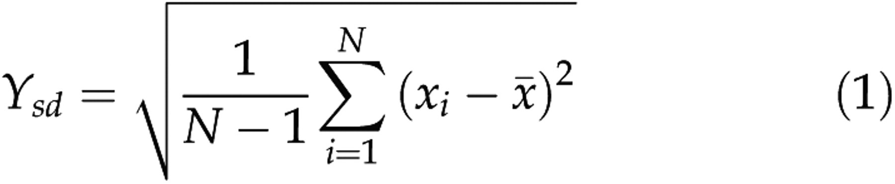
Standard deviation:

where ;

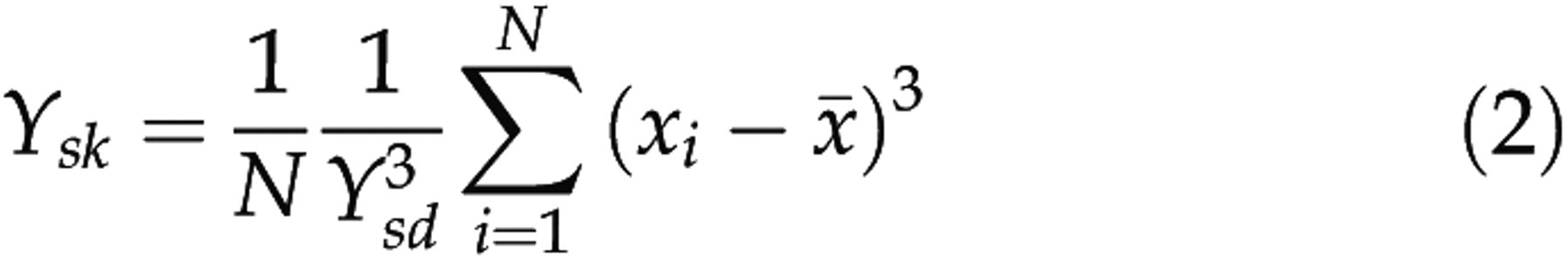
Skewness:

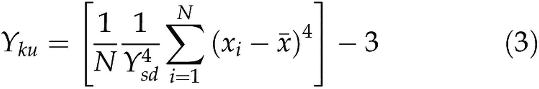
Fisher's kurtosis:

Number of zero crossing (Y _zc), the number of changes of sign of x _i

Number of relative maxima and minima (Y _mm), the number of maxima and minima of x _i

Power spectral densities of the δ band (Y _δ, 0.5–6 Hz) and the θ band (Y _θ, 6–10 Hz).
The first five features were the same as those in the study by Karasinski et al. ⁷ The newly included Y _δ and Y _θ were calculated by Welch's method and they were the means of the values of the corresponding frequencies. The resolution of the power spectral density was 0.5 Hz and the boundaries of the EEG frequency bands were based on the result of principal component analysis of EEG in the rat.¹⁴ For each case of calculation of the five and seven features, respectively, the final result for each rat and each bipolar electrode was represented as {Y _pi ^s}, where p ∈ {five or seven different variables}, s ∈ {Wake, REM, NREM}, i = 1 … M _s, 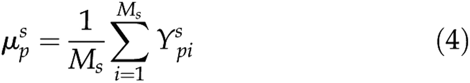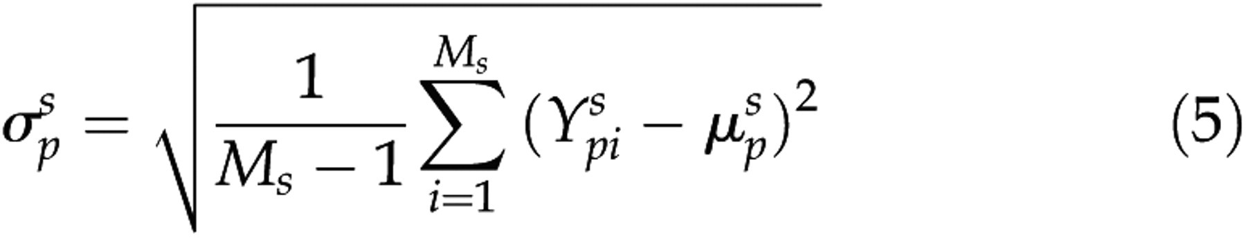where M _s was the number of the representative epochs for a vigilance state. For each rat and each bipolar electrode, the means (μ) and standard deviations (SD, σ) of the five or the seven parameters for the selected representative waves of each vigilance state were calculated as

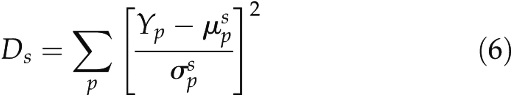
For the raw EEG signals acquired from the two bipolar electrodes, the data preprocessing was the same as that for the representative waves. The data were then divided into epochs of 8 s and epochs were discarded as artefacts when classified as Wake or REM by the two raters, and when their standard deviations were 1.4 times as large as the maximum of standard deviations of the Wake or REM representative waves, respectively. Then the five or the seven parameters (Y _p) were calculated and the normalized distance between Y _p and each of the typical vigilances was calculated by equation (6)

where p ∈ {five or seven different variables}, s ∈ {Wake, REM, NREM} and the epoch was classified to the same typical state with the smallest distance.⁷

Visual scoring by raters (EEG and EMG)

According to the generally recognized criteria,² i.e. low-amplitude, high-frequency EEG accompanied by high-level EMG during the Wake stage, high-amplitude EEG associated with low EMG during NREM sleep, and EEG comprised mainly of θ band and accompanied by flat EMG during REM sleep, two independent raters analysed the 22 h EEG and EMG recordings of five rats for each bipolar electrode, respectively. Before visual scoring, raters reviewed the representative waves used in the above algorithms. They were confident about distinguishing subtle classification criteria for different animals and different channels.

To reduce the influence of human subjectivity, the following three steps were taken. First, for each rat, the channels of the signal acquisition system were assigned randomly for the two bipolar electrodes, so that the raters did not know the corresponding anatomical coordinate of a recording when they were engaged in visual scoring or selecting the representative waves. Second, the two raters reviewed the data independently. Finally, each rater classified the data of a given rat from the two channels in two consecutive days and hence improved the reliability.

Computer method 1 (M1, EEG only)

The data preprocessing of the raw EEG signals acquired from E1 and E2 was the same as that for the representative waves with a band-pass filter from 0.5 to 30 Hz. The seven features (Y _sd, Y _sk, Y _ku, Y _zc, Y _mm, Y _δ and Y _θ) were calculated in order to classify the artefact-free epochs to corresponding states using equation (6).

Computer method 2 (M2, EEG only)

The raw EEG signals acquired from E1 and E2 were analysed by the algorithm (M2) developed by Karasinski et al. The differences between M1 and M2 were the filter bands, 0.5–30 Hz for M1 but 3.18–25 Hz for M2; and the number of parameters, seven for M1 but only five for M2.

Difference in the EEG features between E1 and E2

To check the difference in the EEG features between E1 and E2, we calculated the means (ν) and standard deviations (τ) of each parameter in different vigilance states of the five rats for each bipolar electrode. Each parameter from each bipolar electrode of a rat in each vigilance state was obtained from its 400 s representative waves. The difference in the EEG features between E1 and E2 was determined using the statistical test with ‘combination between algorithm and bipolar electrode’ as the variable.

Statistical analyses

Results from the four combinations (M1E1, M1E2, M2E1 and M2E2) were analysed using two-way within-subject analysis of variance (ANOVA) (i.e. 2-way repeated-measures ANOVA) with the factors ‘rater’ and ‘combination’, and both main effects and interactions were examined. To determine the difference in the EEG features between E1 and E2, results of EEG features in each vigilance state were analysed using the paired-samples t-test or the one-way repeated-measures ANOVA with the factor ‘combination’. For significant ANOVAs, data were further analysed for multiple comparisons using Tukey's post hoc test. In both one-way and two-way ANOVAs, the values of epsilon (ϵ) of Greenhouse–Geisser would be denoted when Greenhouse–Geisser correction was necessary. Effect size estimates for t-tests and ANOVAs were determined with Cohen's d and partial η ², respectively (Cohen's d or partial η ² = 0.20 is a small effect size, 0.50 is a medium effect size and 0.80 is a large effect size).¹⁵ For each case, the kappa statistical parameter, κ, which estimates the overall agreement beyond chance between the computer and each rater or the two raters, was computed. A significance level of P < 0.05 was used in all comparisons.

Results

In this study, we tested two algorithms (M1 and M2) and two bipolar cortical electrodes (E1 and E2). A further processing step was implemented to eliminate REM sleep epochs appearing in Wake, i.e. an epoch was only identified as REM after three NREM epochs, but not after five Wake epochs.⁷ A comparative study was then implemented between the results of the computer and visual scoring (rater). Finally, all the results of five rats (22 h data for each rat) were categorized according to different electrodes and different algorithms. The agreements shown in Tables 1 –4 were calculated over the pooled classification results of the five rats. In Table 5, the agreements between a rater and the computer were first calculated for each rat, and then the means and standard deviations were calculated from the agreements of the five rats. All the data shown in Tables 1 –5 were based on artefact-free epochs, except for the data in Table 4 which were additionally based on consensus epochs for which the two raters gave the same classification. Table 6 shows the differences in EEG properties among the four combinations.

Table 1
Matrix of concordance between the two raters when the pooled classification results of five rats (22 h data for each rat) were used for each bipolar electrode

Rater 1 Rater 2
Rater 2

Wake NREM REM Total %Agree Wake NREM REM Total %Agree

E1 (κ = 0.949) E2 (κ = 0.932)

Wake 23,909 600 80 24,589 97.2 22,158 411 215 22,784 97.3

NREM 391 19,667 120 20,178 97.5 777 20,437 127 21,341 95.8

REM 27 138 2821 2986 94.5 99 155 2641 2895 91.2

Total 24,327 20,405 3021 47,753 23,034 21,003 2983 47,020

%Agree 98.3 96.4 93.4 97.2 96.2 97.3 88.5 96.2

Only artefact-free epochs were used in the analysis. NREM = non-rapid eye movement; REM = rapid eye movement

Table 2
Matrix of concordance between rater 1 and the computer when the pooled classification results of five rats (22 h data for each rat) were used for each combination

Rater 1 Computer
Computer

Wake NREM REM Total %Agree Wake NREM REM Total %Agree

M1E1 (κ = 0.945) M1E2 (κ = 0.875)

Wake 23,800 467 322 24,589 96.8 21,371 644 769 22,784 93.8

NREM 330 19,709 139 20,178 97.7 1122 19,802 417 21,341 92.8

REM 92 118 2776 2986 93.0 160 196 2539 2895 87.7

Total 24,222 20,294 3237 47,753 22,653 20,642 3725 47,020

%Agree 98.3 97.1 85.8 96.9 94.3 95.9 68.2 93.0

M2E1 (κ = 0.888) M2E2 (κ = 0.892)

Wake 22,627 1542 420 24,589 92.0 21,399 974 411 22,784 93.9

NREM 167 19,865 146 20,178 98.4 564 20,695 82 21,341 97.0

REM 256 437 2293 2986 76.8 350 417 2128 2895 73.5

Total 23,050 21,844 2859 47,753 22,313 22,086 2621 47,020

%Agree 98.2 90.9 80.2 93.8 95.9 93.7 81.2 94.0

Only artefact-free epochs were used in the analysis. NREM = non-rapid eye movement; REM = rapid eye movement

Table 3
Matrix of concordance between rater 2 and the computer when the pooled classification results of five rats (22 h data for each rat) were used for each combination

Rater 2 Computer
Computer

Wake NREM REM Total %Agree Wake NREM REM Total %Agree

M1E1 (κ = 0.935) M1E2 (κ = 0.873)

Wake 23,602 461 264 24,327 97.0 21,504 823 707 23,034 93.4

NREM 463 19,699 243 20,405 96.5 927 19,604 472 21,003 93.3

REM 157 134 2730 3021 90.4 222 215 2546 2983 85.4

Total 24,222 20,294 3237 47,753 22,653 20,642 3725 47,020

%Agree 97.4 97.1 84.3 96.4 94.9 95.0 68.3 92.8

M2E1(κ = 0.886) M2E2 (κ = 0.873)

Wake 22,489 1477 361 24,327 92.4 21,273 1313 448 23,034 92.4

NREM 258 19,943 204 20,405 97.7 550 20,354 99 21,003 96.9

REM 303 424 2294 3021 75.9 490 419 2074 2983 69.5

Total 23,050 21,844 2859 47,753 22,313 22,086 2621 47,020

%Agree 97.6 91.3 80.2 93.7 95.3 92.2 79.1 92.9

Only artefact-free epochs were used in the analysis. NREM = non-rapid eye movement; REM = rapid eye movement

Table 4
Matrix of concordance between the computer and the raters when the pooled classification results on consensus epochs of five rats (22 h data for each rat) were used for each combination

Raters Computer
Computer

Wake NREM REM Total %Agree Wake NREM REM Total %Agree

M1E1 (κ = 0.966) M1E2 (κ = 0.905)

Wake 23,413 257 239 23,909 97.9 21,026 500 632 22,158 94.9

NREM 143 19,435 89 19,667 98.8 675 19,434 328 20,437 95.1

REM 76 62 2683 2821 95.1 109 148 2384 2641 90.3

Total 23,632 19,754 3011 46,397 21,810 20,082 3344 45,236

%Agree 99.1 98.4 89.1 98.1 96.4 96.8 71.3 94.7

M2E1 (κ = 0.911) M2E2 (κ = 0.915)

Wake 22,376 1187 346 23,909 93.6 20,927 839 392 22,158 94.4

NREM 66 19496 105 19667 99.1 245 20155 37 20,437 98.6

REM 234 336 2251 2821 79.8 297 314 2030 2641 76.9

Total 22676 21019 2702 46397 21469 21308 2459 45236

%Agree 98.7 92.8 83.3 95.1 97.5 94.6 82.6 95.3

Only artefact-free and consensus epochs were used in the analysis. NREM = non-rapid eye movement; REM = rapid eye movement

Table 5
Comparative results of the consistency of performance for different combinations

Computer Rater
Rater

Rater 1 Rater 2 Average Rater 1 Rater 2 Average

M1E1 M1E2

Wake (%) 96.8 ± 1.1 96.9 ± 1.1 96.9 ± 1.1 93.9 ± 1.6 93.3 ± 1.5 93.6 ± 1.6

NREM (%) 97.6 ± 1.2 96.5 ± 1.5 97.1 ± 1.4 93.0 ± 3.3 93.3 ± 3.1 93.2 ± 3.2

REM (%) 92.7 ± 2.2 90.1 ± 2.7 91.4 ± 2.5 87.7 ± 4.8 85.2 ± 3.6 86.5 ± 4.2

Overall (%) 96.9 ± 0.4 96.4 ± 0.9 96.7 ± 0.7 93.0 ± 1.7 92.9 ± 1.7 93.0 ± 1.7

M2E1 M2E2

Wake (%) 92.0 ± 2.9 92.3 ± 2.5 92.2 ± 2.7 93.5 ± 3.8 91.9 ± 4.7 92.7 ± 4.3

NREM (%) 98.4 ± 1.0 97.7 ± 0.9 98.1 ± 1.0 96.8 ± 2.5 96.6 ± 3.7 96.7 ± 3.1

REM (%) 76.7 ± 5.7 75.9 ± 5.4 76.3 ± 5.6 73.5 ± 1.7 69.3 ± 5.8 71.4 ± 3.8

Overall (%) 93.8 ± 1.5 93.7 ± 1.4 93.8 ± 1.5 94.0 ± 1.2 93.3 ± 1.6 93.7 ± 1.4

Only artefact-free epochs were used in the analysis. For each combination and each rater, the means and standard deviations of agreements between the rater and the computer of five rats were calculated for the three vigilance states respectively and globally. Values in the Average column were the means of the corresponding values between the two raters. All values were denoted as means ± SD. NREM = non-rapid eye movement; REM = rapid eye movement

Table 6
Statistical results of seven parameters in different vigilance states

Wake NREM REM

Y _δ P 0.043* 0.688 0.024*

Cohen's d 0.87^† 0.26^‡ 1.45^†

M1E1 > M1E2 M1E1 > M1E2

Y _θ P 0.550 0.062 0.386

Cohen's d 0.33^‡ 1.79^† 0.46^‡

F(3,12) 20.447 (ϵ = 0.341) 30.655 (ϵ = 0.415) 4.866 (ϵ = 0.336)

Y _sd P 0.010* 0.002* 0.092

Partial η ² 0.836^† 0.885^† 0.549^¶

Tukey's test M1E1,M1E2 > M2E1,M2E2 M1E1,M1E2,M2E1 > M2E2

M1E1,M1E2 > M2E1

F(3,12) 26.410 22.091 119.261

Y _sk P 0.000 0.000 0.000

Partial η ² 0.868^† 0.847^† 0.968^†

Tukey's test M2E2 > M1E1,M1E2,M2E1 M1E1,M1E2,M2E2 > M2E1 M2E1,M2E2 > M1E1,M1E2

M2E1 > M1E1,M1E2 M1E2 > M2E2

F(3,12) 20.676 14.366 48.305 (ϵ = 0.536)

Y _ku P 0.000 0.000 0.000

Partial η ² 0.838^† 0.782^¶ 0.924^†

Tukey's test M1E1,M1E2,M2E1 > M2E2 M2E1 > M1E1,M1E2,M2E2 M1E1 > M1E2,M2E1,M2E2

M1E1 > M2E1 M1E2,M2E1 > M2E2

F(3,12) 41.093 273.067 49.135

Y _zc P 0.000 0.000 0.000

Partial η ² 0.911^† 0.986^† 0.925^†

Tukey's test M2E1 > M1E1,M1E2,M2E2 M2E1 > M1E1,M1E2,M2E2 M1E1 > M1E2,M2E1,M2E2

M1E1,M2E2 > M1E2 M2E2 > M1E1,M1E2 M2E1 > M1E2,M2E2

M1E1 > M1E2

F(3,12) 527.254 151.836 303.261

Y _mm P 0.000 0.000 0.000

Partial η ² 0.992^† 0.974^† 0.987^†

Tukey's test M1E1 > M1E2,M2E1,M2E2 M1E1 > M1E2,M2E1,M2E2 M1E1 > M1E2,M2E1,M2E2

M1E2 > M2E1,M2E2 M1E2 > M2E1,M2E2 M1E2,M2E1 > M2E2

M2E1 > M2E2 M2E1 > M2E2

This table was derived from the data-sets of 400 s representative waves from each bipolar electrode in each vigilance state of each rat. For the first two parameters, Y _δ and Y _θ, their results in each vigilance state were analysed using the paired-samples t-test. For the other five parameters, their results in each vigilance state were analysed using one-way repeated-measures ANOVA with the factor ‘combination’. The values of epsilon (ϵ) of Greenhouse–Geisser are also denoted in this table when Greenhouse–Geisser correction is necessary. Effect size estimates for t-tests and ANOVAs were determined with Cohen's d and partial η ², respectively (Cohen's d or partial η ² = 0.20 is a small effect size, 0.50 is a medium effect size and 0.80 is large effect size). The symbols ‘>’ denote that the means (ν) of the seven parameters given by the combinations at the left side of ‘>’ are significantly larger than those at the right side, and no significant difference exists among the combinations at the same side of ‘>’ for each case. NREM = non-rapid eye movement; REM = rapid eye movement

*P < 0.05

**P < 0.001

^†Large effect size

^‡Small effect size

^¶Medium effect size

Agreement between rater 1 and rater 2

The overall agreements between rater 1 and rater 2 were 97.2% (κ = 0.949, P < 0.001) and 96.2% (κ = 0.932, P < 0.001) for E1 and E2, respectively (Table 1, 22 h data for each rat).

Agreement between rater 1 and the computer

The overall agreements between rater 1 and the computer were 96.9% (κ = 0.945, P < 0.001), 93.0% (κ = 0.875, P < 0.001), 93.8% (κ = 0.888, P < 0.001) and 94.0% (κ = 0.892, P < 0.001) for M1E1, M1E2, M2E1 and M2E2, respectively. For each combination, the agreements for Wake and NREM were much better than those for REM, while REM sleep was generally overestimated by the computer. However, for the four combinations, M1E1 showed the best agreement (Table 2, 22 h data for each rat).

Agreement between rater 2 and the computer

The overall agreements between rater 2 and the computer were 96.4% (κ = 0.935, P < 0.001), 92.8% (κ = 0.873, P < 0.001), 93.7% (κ = 0.886, P < 0.001) and 92.9% (κ = 0.873, P < 0.001) for M1E1, M1E2, M2E1 and M2E2, respectively. The results for Wake and NREM were also much better than those for REM. Again REM sleep was overestimated by the computer, and M1E1 was the best of the four combinations (Table 3, 22 h data for each rat).

Performance of different combinations

Table 4, derived from 22 h data for each rat, shows concordance between the computer and the raters when the pooled classification results of consensus epochs, for which the two raters gave the same classification, were used for each bipolar electrode. The overall agreements between the computer and the raters were 98.1% (κ = 0.966, P < 0.001), 94.7% (κ = 0.905, P < 0.001), 95.1% (κ = 0.911, P < 0.001) and 95.3% (κ = 0.915, P < 0.001) for M1E1, M1E2, M2E1 and M2E2, respectively. The accuracies of Wake and NREM for M1E2, M2E1 and M2E2 were much higher than those of REM, and REM sleep was overestimated by the computer. For M1E1, though the accuracies of Wake and NREM were almost as high as the other combinations, the accuracy of REM was much higher than that of the others. Thus, it is reasonable to conclude that M1E1 is the best of the four.

Table 5 shows the means and the standard deviations of the accuracies of the data from the five rats for each combination, vigilance state and rater. For Wake and REM stages, the means of accuracies from M1E1 were the largest, and the standard deviations of accuracies of M1E1 were the smallest. M2E1 performed a little better than M1E1 did for NREM. However, if applied to all the three vigilance stages, M1E1 is still considered to be the most accurate combination (Table 5).

Statistical results of agreements between raters and the computer for the four combinations

The results of agreements between raters and the computer were analysed by ANOVA: (1) no significant difference was found in accuracies between the two raters (P > 0.05); (2) for Wake (F(3,12) = 6.018, Greenhouse–Geisser ϵ = 0.490; P < 0.05, partial η ² = 0.601), REM (F(3,12) = 37.015, P < 0.001, partial η ² = 0.902) and Overall (F(3,12) = 22.398, P < 0.001, partial η ² = 0.848), the main effects of the factor ‘combination’ were all significant and effect sizes for both REM and Overall were large in contrast to the medium effect size for Wake; (3) for Wake, the accuracy of M1E1 was significantly higher than that of M2E1 and M2E2 (Tukey's test, P < 0.05); (4) for REM, the accuracies of both M1E1 and M1E2 were significantly higher than those of M2E1 and M2E2 (Tukey's test, P < 0.05); and (5) for Overall, the accuracy of M1E1 was significantly higher than that of M1E2, M2E1 and M2E2 (Tukey's test, P < 0.05).

Difference in the EEG features among the four combinations

For each combination, the means (ν) and standard deviations (τ) of each parameter (7 and 5 parameters) in each vigilance state obtained from its 400 s representative waves over the five rats are shown in Figure 2.

Figure 2
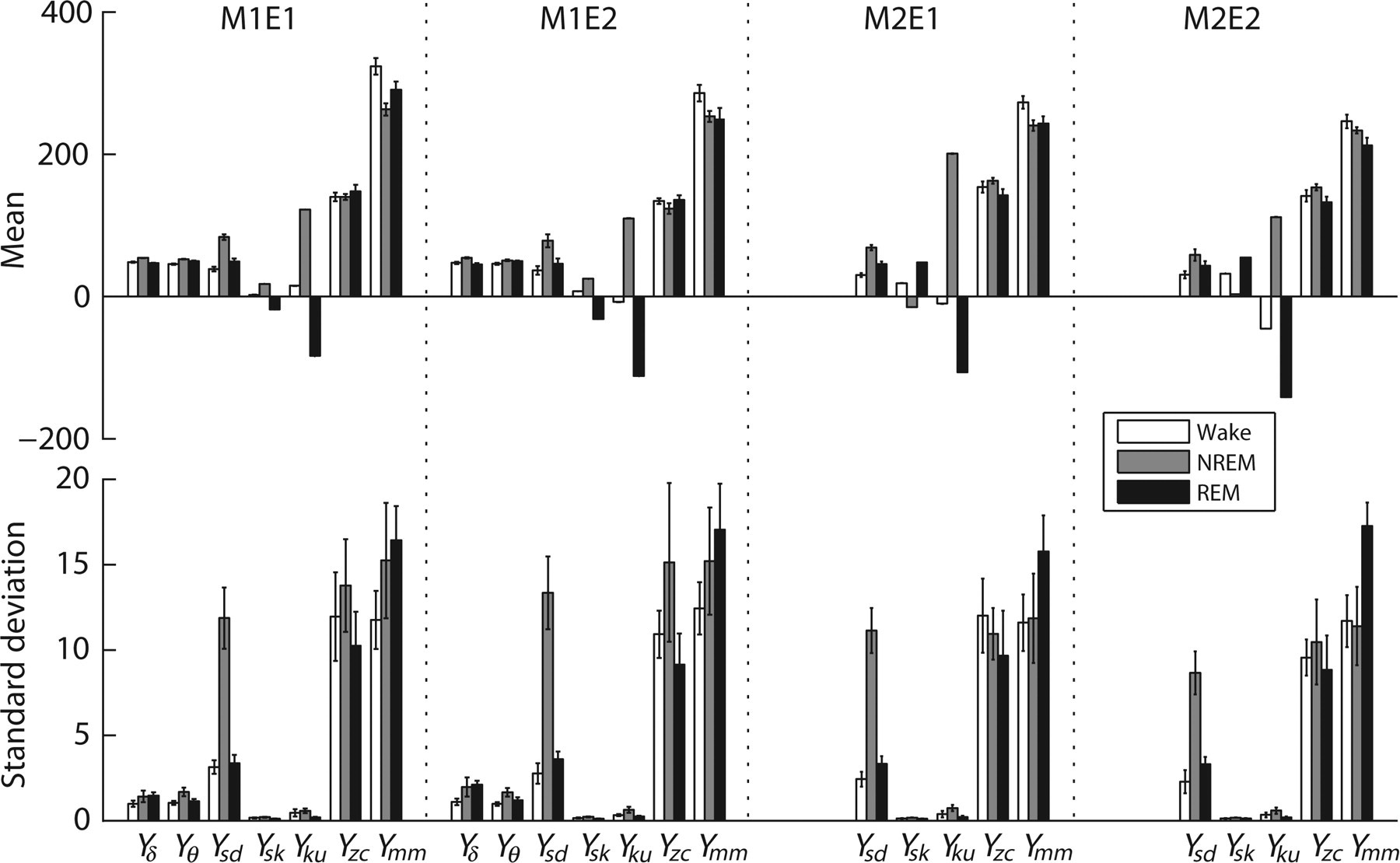
Means (ν) and standard deviations (τ) of seven and five parameters of sleep EEG for the three different vigilance states and for the four combinations. These parameters for each combination of a rat in each vigilance state were obtained from its 400 s representative waves. The means (ν) and standard deviations (τ) of each parameter for the five rats were calculated and plotted. The means of Y _sk and Y _ku were quite low; so they were multiplied by 200 for a better demonstration. The top row denotes the means (ν) of the seven and the five parameters in each vigilance state for M1E1, M1E2, M2E1 and M2E2. The bottom row denotes the standard deviations (τ) of the seven and the five parameters in each vigilance state for M1E1, M1E2, M2E1 and M2E2. Y _δ = power spectral density of the δ band; Y _θ = power spectral density of the θ band; Y _sd = standard deviation; Y _sk = skewness; Y _ku = kurtosis; Y _zc = number of zeros crossing; Y _mm = number of relative maxima and minima; EEG = electroencephalogram; REM = rapid eye movement; NREM = non-rapid eye movement

For each vigilance state and each parameter, different combinations gave significantly different results, with the exception of Y _δ in NREM (P > 0.05), Y _θ in each vigilance state (P > 0.05) and Y _sd in REM (F(3,12) = 4.866, Greenhouse–Geisser ϵ = 0.336; P > 0.05) (Table 6). Each case with significant difference had a large effect size, except Y _ku in NREM, which had medium effect size.

Discussion

This work aims at improving a sleep staging strategy using a single EEG channel and a non-threshold-based algorithm for the long-term study of sleep in rats. We test two different bipolar electrodes (E1, E2) and two different algorithms (M1, M2), with one combination (M2E2) being the same as that in the study by Karasinski et al. The results illustrate that although the overestimations of REM epochs exist more or less in the four combinations, M1E1 is the best solution when applied to all the three vigilance stages. However, it should be noted that Robert et al. have developed an algorithm based on artificial neural networks and thresholds to the same data of the study⁷ by Karasinski et al., and the results are 95.31 ± 1.06% for Wake, 97.43 ± 1.66% for NREM and 92.33 ± 2.27% for REM.⁸ This result indicates that the accuracy for REM sleep of the study by Karasinski et al. can be improved admirably by developing sleep-staging algorithm. In our study, the agreements between the computer and two independent raters for M1E1 were 96.9 ± 1.1% for Wake, 97.1 ± 1.4% for NREM and 91.4 ± 2.5% for REM (Table 5). Both the accuracies for NREM and REM of our study were a little lower than those of the study by Robert et al. ⁸ These works confirm that, on the one hand, even with a single EEG channel, the sleep staging of the rat could be realized at an accuracy comparable to that with both EEG and EMG^1,5 and on the other, the improvement of accuracy could be realized through various strategies. Because the present study focused on sleep staging strategy using a single EEG channel and a non-threshold-based algorithm, the comparisons reported below were mainly restricted to the differences between the scheme by Karasinski et al. and ours because both of them were non-threshold-based methods.

Most agreements, especially those of REM, between rater 1 and rater 2 from E2 were slightly lower than those from E1 (Table 1), and this fact showed that the raw signals from E2 were a little more difficult for visual scoring than those from E1. The discrepancies between the two raters were seen mainly in the classification on transitions, probably due to different individual experiences and the understandings of the criteria for classification. Anyway, the transitions were indeed difficult for the raters to classify, so the minor discrepancies were quite understandable.

In this study, we compared a fronto-parietal location (E1) with the parieto-cerebellar location (E2), which Karasinski et al. ⁷ selected in EEG acquisition. Our idea was based on the following fact: sleep spindles and slow-wave activity (SWA; EEG power between 0.5 and 4.0 Hz, mainly reflecting the δ waves) are the typical waves during NREM sleep, and the optimized electrode placements for these waves are over the frontal and parietal cortex.^16,17 Furthermore, although interhemispheric sleep EEG asymmetry had not been found in the frontal cortex,¹² the waking EEG in complex behavioural tasks and the NREM sleep EEG after complex behavioural tasks showed significant, substantial power increase in the frontal hemisphere contralateral to the dominant paw.¹⁸ As rats may have different handedness, an electrode on the midline could generally balance the interhemispheric EEG asymmetry caused by handedness and reduce its effect on sleep staging. So a frontal midline point was selected as one site of our electrode pair. To choose the best frontal electrode, our previous study was made with four different frontal sites in 10 rats by using M1, and the results illustrate that the frontal midline point (+4, 0L) is the best.¹⁹ During REM sleep, the EEG is comprised of very regular waves with a dominant frequency of the θ band.^2,6,11 Since θ oscillations originate in the hippocampus and several extrahippocampal regions,²⁰ and power in the θ band exhibits a right-hemispheric predominance,¹² we selected the other site of our electrode pair above the right hippocampus (−3.8P, −2L).

The original method (M2) set the band-pass filter from 3.18 to 25 Hz; however, such a choice ignores the contribution of the low frequencies (0–3.18 Hz); in other words, it omits about half of the δ band (0.5–6 Hz).⁶ As the δ band is one of the typical waveforms during NREM sleep,^2,6,11 the new algorithm (M1) with band-pass filter from 0.5 to 30 Hz would likely improve the accuracies of sleep staging by covering wider EEG frequencies. M2 introduces only five parameters; in M1, however, two more parameters (the power spectral densities of the δ band and the θ band) are considered. In fact, either the δ band or the θ band, its amplitude in one of the vigilance states is significantly different from the amplitude in the other two states, respectively.² Therefore, these two parameters may help to discriminate different states of the brain. In fact, it is M1E1 with seven parameters that gives the best result.

Matrices among the computer and the raters in different conditions, and the difference in the EEG features over the four combinations illustrated that the accuracies of sleep staging were improved by the optimizations of the algorithm and the coordinates of the electrode pair (Tables 2 –6 and Figure 2). The most distinct improvement was in the accuracy of REM sleep staging. The agreement between raters and the computer (M2E2) on consensus epochs was 96.0% for Wake, 97.1% for NREM and 83% for REM in the study by Karasinski et al., but the agreement was 97.9% for Wake, 98.8% for NREM, 95.1% for REM and 98.1% for the Overall agreement in our study (Table 4, M1E1). In fact, if we adopted the same electrode and algorithm (M2E2) as Karasinski et al., the agreement between raters and the computer on consensus epochs would be 94.4% for Wake, 98.6% for NREM and 76.9% for REM (Table 4, M2E2), which would be closed to the result reported by Karasinski et al. Such a fact indicates that the comparative studies are objective and creditable.

The results suggest that (1) different algorithms would result in different accuracies of sleep staging; (2) different electrode placement would induce differences in raw data and hence affect the accuracy of sleep staging, with a milder effect than that caused by different algorithms though. So if good accuracy of sleep staging were to be achieved, a suitable algorithm with corresponding optimum electrode locations would be necessary.

EEG has been found to be different at various regions and sleep stages in rats, and the changes of low-frequency EEG differ along the anteroposterior and left–right axes.¹² For example, the δ power spectral densities in both Wake and REM were significantly different between E1 and E2 (Figure 2 and Table 6). In fact, it is now widely accepted that sleep is not only a global process but also has a local use-dependent component that is manifested as regional differences in SWA.^21,22 Oscillations about 3 Hz (SWA) were prominent in the most rostral regions of the anterior midline cortex including the medial prefrontal region (mPFC, under the frontal electrode of E1), and the δ band power was significantly different between the anterior and posterior halves of the cortex (including the hippocampus).²³ Furthermore, the absolute mean power of cerebellar activity is several folds lower than that at the cerebral level;²⁴ cerebellum (under the cerebellar electrode of E2) as referenced was more like a rest reference at infinity than other cortexes. As EEG data acquired from a bipolar electrode is the difference between two electrodes, and the two parietal electrodes in our study were very close to each other, E1 may have collected more δ information than E2 (Table 6).

As shown in Figure 2, the changes of EEG parameters were quite similar between data acquired from the two bipolar electrodes, and this phenomenon illustrates that EEGs highly correlate with each other between channels. But many significant differences could be found among the four combinations by statistical tests (Table 6), and such differences resulted from different bipolar electrodes (e.g. Y _δ in Wake and REM), different algorithms (e.g. Y _sd in Wake) and different combinations of bipolar electrodes and algorithms (e.g. Y _mm in Wake, NREM and REM). It is these differences that resulted in the different accuracies of sleep staging among the four combinations. In summary, E1 produced more EEG information than E2, and M1 made the most of the data; so M1E1 was the optimized combination for sleep scoring.

Although θ activities have been recorded locally from several extrahippocampal regions,²⁰ they are generally believed to originate mainly from the hippocampus in rodents.²⁵ On the one hand, the hippocampal θ rhythm in rats appears with striking regularity when the animals engage in exploratory behaviour, which includes movement, sniffing and orienting, and in REM sleep.²⁵ Hippocampal θ activities fall into two different categories: movement-related (Type I, with a frequency range of 7–12 Hz), which is observed with walking and rearing; and immobility-related (Type II, with a frequency range of 4–9 Hz), which is associated with grooming, alert immobility and REM sleep.^23,25–27 Cortical θ oscillations in rats are observed during wakefulness and REM,^23,28,29 and these oscillations are also behaviour-dependent during the awake state as the hippocampal θ rhythm (Type I and Type II).²³ So it can be deduced that the hippocampal θ rhythm and the cortical θ rhythm are similar during wakefulness or REM. On the other hand, simultaneous cellular recording in the hippocampus and recordings of cortical and hippocampal field potentials have elucidated the cellular mechanisms of the θ rhythm and proved the relationship between frequency of θ oscillations and firing frequency of the θ cells.^25,30 Furthermore, it has been demonstrated that the cortical θ is closely coupled with the hippocampal θ rhythm.^23,31 In other words, even though there may be some other θ origins besides the hippocampus, the cortical θ and the hippocampal θ are tightly correlative, thus the hippocampal θ rhythm can be represented by the cortical θ rhythm. In the present study, the hippocampal θ rhythm itself could not be recorded directly using the electrodes employed by us, but the cortical θ activity, which was highly relevant to the hippocampal θ rhythm,^23,31 could be recorded by our fronto-parietal electrode.

Because there are similar cortical and hippocampal Type II θ activities in both Wake and REM sleep,^23,25–27 the representative waves of REM sleep are similar to the θ signals in Wake with grooming and alert immobility. Consequently, the epochs in Wake with grooming and alert immobility could be easily mistaken as REM. This is the reason for the overestimation of REM sleep. But because the amplitude of the θ band in REM sleep is significantly different from those in the other two states² and because significantly different electrophysiological features of EEG in other frequency bands during different vigilance states exist, the disadvantage about overestimation of REM sleep may be reduced by more accurate selection of the representative wave. In fact, overestimation of REM sleep did not exist in the study by Karasinski et al. ⁷ We speculate it may be that they used a different method to select the representative wave. They selected the most typical representative waves from the results calculated by the five parameters while we selected them from raw EEG and EMG recordings. Although these overestimations exist in the four combinations, the overestimation in M1E1 is very low (Table 4). So M1E1 is suitable for the long-term study of sleep because of its non-threshold-based method and single use of EEG recording.⁷

On the one hand, however, it should be noted that the present study was based only on healthy normal animals under baseline conditions without any manipulations or pharmacological treatments. As pharmacological treatments may induce dissociation between the EEG and the behaviour of the animal,⁶ and the properties of an unhealthy rat EEG may be different from a healthy rat; so the classification accuracies of sleep staging will decline when the method M1E1 is used under the conditions different from those in this study, such as unhealthy rats, manipulations and pharmacological treatments. In general, the current clustering method with data from E1 (M1E1) is suitable for the long-term study of sleep, especially in studies on circadian rhythmic mechanisms of the sleep–wake cycle under baseline conditions without manipulations or pharmacological treatments. On the other hand, the results reported above were only from 22 h recordings instead of the whole 24 h recordings, i.e. the 2 h data from the light–dark change was omitted in this study. Since there are many transitions during the light–dark change, and the epochs of transitions are difficult to classify correctly, exclusion of the 2 h data would also affect the evaluation of various methods (M1E1 and M2E2), and the classification accuracies of sleep staging for M1E1 would decline when this method is used for 24 h recordings, especially under drug or behavioural manipulations in which the number of transitions increases dramatically.

In summary, comparative studies were carried out across two different non-threshold-based algorithms using EEG only and two different sets of coordinates of electrodes. Our results indicate that the accuracies of sleep staging, especially for REM sleep, could be improved by increasing classification parameters, optimizing the band-pass filters and the coordinates of an electrode pair for a single EEG channel. These results also show that different algorithms and different electrode placements will lead to significantly different accuracies of sleep scoring. To obtain good accuracy of sleep staging, we need not only a robust algorithm on typical features, but also an optimum electrode placement to get crucial physiological information related to sleep. Our results show that the new method (M1E1) can be realized easily and is suitable for the long-term study of sleep.

Rater 1	Rater 2	Rater 2
	E1 (κ = 0.949)	E2 (κ = 0.932)
Wake	23,909	600	80	24,589	97.2	22,158	411	215	22,784	97.3
NREM	391	19,667	120	20,178	97.5	777	20,437	127	21,341	95.8
REM	27	138	2821	2986	94.5	99	155	2641	2895	91.2
Total	24,327	20,405	3021	47,753		23,034	21,003	2983	47,020
%Agree	98.3	96.4	93.4		97.2	96.2	97.3	88.5		96.2

Rater 1	Computer	Computer
	M1E1 (κ = 0.945)	M1E2 (κ = 0.875)
Wake	23,800	467	322	24,589	96.8	21,371	644	769	22,784	93.8
NREM	330	19,709	139	20,178	97.7	1122	19,802	417	21,341	92.8
REM	92	118	2776	2986	93.0	160	196	2539	2895	87.7
Total	24,222	20,294	3237	47,753		22,653	20,642	3725	47,020
%Agree	98.3	97.1	85.8		96.9	94.3	95.9	68.2		93.0
	M2E1 (κ = 0.888)	M2E2 (κ = 0.892)
Wake	22,627	1542	420	24,589	92.0	21,399	974	411	22,784	93.9
NREM	167	19,865	146	20,178	98.4	564	20,695	82	21,341	97.0
REM	256	437	2293	2986	76.8	350	417	2128	2895	73.5
Total	23,050	21,844	2859	47,753		22,313	22,086	2621	47,020
%Agree	98.2	90.9	80.2		93.8	95.9	93.7	81.2		94.0

Rater 2	Computer	Computer
	M1E1 (κ = 0.935)	M1E2 (κ = 0.873)
Wake	23,602	461	264	24,327	97.0	21,504	823	707	23,034	93.4
NREM	463	19,699	243	20,405	96.5	927	19,604	472	21,003	93.3
REM	157	134	2730	3021	90.4	222	215	2546	2983	85.4
Total	24,222	20,294	3237	47,753		22,653	20,642	3725	47,020
%Agree	97.4	97.1	84.3		96.4	94.9	95.0	68.3		92.8
	M2E1(κ = 0.886)	M2E2 (κ = 0.873)
Wake	22,489	1477	361	24,327	92.4	21,273	1313	448	23,034	92.4
NREM	258	19,943	204	20,405	97.7	550	20,354	99	21,003	96.9
REM	303	424	2294	3021	75.9	490	419	2074	2983	69.5
Total	23,050	21,844	2859	47,753		22,313	22,086	2621	47,020
%Agree	97.6	91.3	80.2		93.7	95.3	92.2	79.1		92.9

Raters	Computer	Computer
	M1E1 (κ = 0.966)	M1E2 (κ = 0.905)
Wake	23,413	257	239	23,909	97.9	21,026	500	632	22,158	94.9
NREM	143	19,435	89	19,667	98.8	675	19,434	328	20,437	95.1
REM	76	62	2683	2821	95.1	109	148	2384	2641	90.3
Total	23,632	19,754	3011	46,397		21,810	20,082	3344	45,236
%Agree	99.1	98.4	89.1		98.1	96.4	96.8	71.3		94.7
	M2E1 (κ = 0.911)	M2E2 (κ = 0.915)
Wake	22,376	1187	346	23,909	93.6	20,927	839	392	22,158	94.4
NREM	66	19496	105	19667	99.1	245	20155	37	20,437	98.6
REM	234	336	2251	2821	79.8	297	314	2030	2641	76.9
Total	22676	21019	2702	46397		21469	21308	2459	45236
%Agree	98.7	92.8	83.3		95.1	97.5	94.6	82.6		95.3

Computer	Rater	Rater
	M1E1	M1E2
Wake (%)	96.8 ± 1.1	96.9 ± 1.1	96.9 ± 1.1	93.9 ± 1.6	93.3 ± 1.5	93.6 ± 1.6
NREM (%)	97.6 ± 1.2	96.5 ± 1.5	97.1 ± 1.4	93.0 ± 3.3	93.3 ± 3.1	93.2 ± 3.2
REM (%)	92.7 ± 2.2	90.1 ± 2.7	91.4 ± 2.5	87.7 ± 4.8	85.2 ± 3.6	86.5 ± 4.2
Overall (%)	96.9 ± 0.4	96.4 ± 0.9	96.7 ± 0.7	93.0 ± 1.7	92.9 ± 1.7	93.0 ± 1.7
	M2E1	M2E2
Wake (%)	92.0 ± 2.9	92.3 ± 2.5	92.2 ± 2.7	93.5 ± 3.8	91.9 ± 4.7	92.7 ± 4.3
NREM (%)	98.4 ± 1.0	97.7 ± 0.9	98.1 ± 1.0	96.8 ± 2.5	96.6 ± 3.7	96.7 ± 3.1
REM (%)	76.7 ± 5.7	75.9 ± 5.4	76.3 ± 5.6	73.5 ± 1.7	69.3 ± 5.8	71.4 ± 3.8
Overall (%)	93.8 ± 1.5	93.7 ± 1.4	93.8 ± 1.5	94.0 ± 1.2	93.3 ± 1.6	93.7 ± 1.4

		Wake	NREM	REM
Y _δ	P	0.043*	0.688	0.024*
	Cohen's d	0.87^†	0.26^‡	1.45^†
		M1E1 > M1E2		M1E1 > M1E2
Y _θ	P	0.550	0.062	0.386
	Cohen's d	0.33^‡	1.79^†	0.46^‡
	F(3,12)	20.447 (ϵ = 0.341)	30.655 (ϵ = 0.415)	4.866 (ϵ = 0.336)
Y _sd	P	0.010*	0.002*	0.092
	Partial η ²	0.836^†	0.885^†	0.549^¶
	Tukey's test	M1E1,M1E2 > M2E1,M2E2	M1E1,M1E2,M2E1 > M2E2
			M1E1,M1E2 > M2E1
	F(3,12)	26.410	22.091	119.261
Y _sk	P	0.000**	0.000**	0.000**
	Partial η ²	0.868^†	0.847^†	0.968^†
	Tukey's test	M2E2 > M1E1,M1E2,M2E1	M1E1,M1E2,M2E2 > M2E1	M2E1,M2E2 > M1E1,M1E2
		M2E1 > M1E1,M1E2	M1E2 > M2E2
	F(3,12)	20.676	14.366	48.305 (ϵ = 0.536)
Y _ku	P	0.000**	0.000**	0.000**
	Partial η ²	0.838^†	0.782^¶	0.924^†
	Tukey's test	M1E1,M1E2,M2E1 > M2E2	M2E1 > M1E1,M1E2,M2E2	M1E1 > M1E2,M2E1,M2E2
		M1E1 > M2E1		M1E2,M2E1 > M2E2
	F(3,12)	41.093	273.067	49.135
Y _zc	P	0.000**	0.000**	0.000**
	Partial η ²	0.911^†	0.986^†	0.925^†
	Tukey's test	M2E1 > M1E1,M1E2,M2E2	M2E1 > M1E1,M1E2,M2E2	M1E1 > M1E2,M2E1,M2E2
		M1E1,M2E2 > M1E2	M2E2 > M1E1,M1E2	M2E1 > M1E2,M2E2
			M1E1 > M1E2
	F(3,12)	527.254	151.836	303.261
Y _mm	P	0.000**	0.000**	0.000**
	Partial η ²	0.992^†	0.974^†	0.987^†
	Tukey's test	M1E1 > M1E2,M2E1,M2E2	M1E1 > M1E2,M2E1,M2E2	M1E1 > M1E2,M2E1,M2E2
		M1E2 > M2E1,M2E2	M1E2 > M2E1,M2E2	M1E2,M2E1 > M2E2
		M2E1 > M2E2	M2E1 > M2E2

Footnotes

Acknowledgements

This research was supported by the National Natural Science Foundation of China (Nos. 60736029, 30870655, 30525030) and the 863 project 2009AA02Z301.

References

Hamrahi

, Chan

, Horner

. On-line detection of sleep-wake states and application to produce intermittent hypoxia only in sleep in rats. J Appl Physiol 2001;90:2130–40

Louis

, Lee

, Stephenson

. Design and validation of a computer-based sleep-scoring algorithm. J Neurosci Methods 2004;133:71–80

Mileva-Seitz

, Louis

, Stephenson

. A visual aid for computer-based analysis of sleep–wake state in rats. J Neurosci Methods 2005;148:43–8

Witting

, van der Werf

, Mirmiran

. An on-line automated sleep–wake classification system for laboratory animals. J Neurosci Methods 1996;2:109–12

Costa-Miserachs

, Portell-Cortés

, Torras-Garcia

, Morgado-Bernal

. Automated sleep staging in rat with a standard spreadsheet. J Neurosci Methods 2003;130:93–101

Robert

, Guilpin

, Limoge

. Automated sleep staging systems in rats. J Neurosci Methods 1999;88:111–22

Karasinski

, Stinus

, Robert

, Limoge

. Real-time sleep–wake scoring in the rat using a single EEG channel. Sleep 1994;17:113–19

Robert

, Karasinski

, Natowicz

, Limoge

. Adult rat vigilance states discrimination by artificial neural networks using a single EEG channel. Physiol Behav 1996;59:1051–60

Van Gelder

, Edgar

, Dement

. Real-time automated sleep scoring: validation of a microcomputer-based system for mice. Sleep 1991;14:48–55

10.

Tang

, Orchard

, Liu

, Sanford

. Effect of varying recording cable weight and flexibility on activity and sleep in mice. Sleep 2004;27:803–10

11.

Bjorvatn

, Fagerland

, Ursin

. EEG power densities (0.5–20 Hz) in different sleep–wake stages in rats. Physiol Behav 1998;63:413–17

12.

Vyazovskiy

, Borbély

, Tobler

. Interhemispheric sleep EEG asymmetry in the rat is enhanced by sleep deprivation. J Neurophysiol 2002;5:2280–6

13.

Abou-Ismail

, Burman

OHP

, Nicol

, Mendl

. Let sleeping rats lie: does the timing of husbandry procedures affect laboratory rat behaviour, physiology and welfare? Appl Anim Behav Sci 2008;111:329–41

14.

Corsi-Cabrera

, Pérez-Garci

, Río-Portilla

, Ugalde

, Guevara

. EEG bands during wakefulness, slow-wave, and paradoxical sleep as a result of principal component analysis in the rat. Sleep 2001;24:374–80

15.

Cohen

. A power primer. Psychol Bull 1992;112:155–9

16.

Calvet

, Fourment

, Thiefry

. Electrical activity in neocortical projection and association areas during slow wave sleep. Brain Res 1973;52:173–87

17.

Terrier

, Gottesmann

. Study of cortical spindles during sleep in the rat. Brain Res Bull 1978;3:701–6

18.

Vyazovskiy

, Tobler

. Handedness leads to interhemispheric EEG asymmetry during sleep in the rat. J Neurophysiol 2008;99:969–75

19.

Fang

, Zhang

, Xia

, The effect of different EEG derivations on sleep staging in rats: the frontal midline-parietal bipolar electrode for sleep scoring. Physiol Meas 2009;30:589–601

20.

Kahana

, Seelig

, Madsen

. Theta returns. Curr Opin Neurobiol 2001;11:739–44

21.

Krueger

, Obál

. A neuronal group theory of sleep function. J Sleep Res 1993;2:63–9

22.

Krueger

, Obál

, Fang

Jr . Why we sleep, a theoretical view of sleep function. Sleep 1999;3:119–29

23.

Young

, Mcnaughton

. Coupling of theta oscillations between anterior and posterior midline cortex and with the hippocampus in freely behaving rats. Cereb Cortex 2009;19:24–40

24.

Culic

, Grbic

, Martac Blanusa

, Spasic

, Jankovic

, Rankovic

. Slow and fast oscillations in the activity of parietal cortex after brain injury. In: Gantchev

, ed. From Basic Motor Control to Functional Recovery III. Sofia: St Kliment Ohridski University Press, 2003

25.

Bland

. The physiology and pharmacology of hippocampal formation theta rhythms. Progr Neurobiol 1986;26:1–54

26.

Vanderwolf

. Hippocampal electrical activity and voluntary movement in the rat. Electroencephalogr Clin Neurophysiol 1969;26:407–18

27.

Vanderwolf

. Neocortical and hippocampal activation in relation to behavior: effects of atropine, eserine, phenotiazines and amphetamine. J Comp Physiol Psychol 1975;88:300–23

28.

Young

, Steinfels

, Khazan

. Cortical EEG power spectra associated with sleep-awake behavior in the rat. Pharmacol Biochem Behav 1978;8:89–91

29.

Marini

, Ceccarelli

, Mancia

. Characterization of the 7–12 Hz EEG oscillations during immobile waking and REM sleep in behaving rats. Clin Neurophysiol 2008;119:315–20

30.

Bland

, Seto

, Rowntree

. The relation of multiple hippocampal theta cell discharge rates to slow wave theta frequency. Physiol Behav 1983;31:111–17

31.

Siapas

, Lubenov

, Wilson

. Prefrontal phase locking to hippocampal theta oscillations. Neuron 2005;46:141–51

Optimized single electroencephalogram channel sleep staging in rats

Abstract

Keywords

Materials and methods

Animals

Surgery

Data acquisition

Data processing

Visual scoring by raters (EEG and EMG)

Computer method 1 (M1, EEG only)

Computer method 2 (M2, EEG only)

Difference in the EEG features between E1 and E2

Statistical analyses

Results

Agreement between rater 1 and rater 2

Agreement between rater 1 and the computer

Agreement between rater 2 and the computer

Performance of different combinations

Statistical results of agreements between raters and the computer for the four combinations

Difference in the EEG features among the four combinations

Discussion

Footnotes

Acknowledgements

References