Sage Journals: Discover world-class research

Abstract

Background

The estimation of breast cancer screening sensitivity is a major aim in the quality assessment of screening programmes. The proportional incidence method for the estimation of the sensitivity of breast cancer screening programmes is rarely used to estimate the underlying incidence rates.

Methods

We present a method to estimate episode and programme sensitivity of screening programmes, based solely on cancers detected within screening cycles (excluding breast cancer cases at prevalent screening round) and on the number of incident cases in the total target population (steady state). The assumptions, strengths and limitations of the method are discussed. An example of calculation of episode and programme sensitivities is given, on the basis of the data from the IMPACT study, a large observational study of breast cancer screening programmes in Italy.

Results

The programme sensitivity from the fifth year of screening onwards ranged between 41% and 48% of the total number of cases in the target population. At steady state episode sensitivity was 0.70, with a trend across age groups, with lowest values in women aged 50-54 years (0.52) and highest in those 65-69 (0.77).

Conclusions

The method is a very serviceable tool for estimating sensitivity in service screening programmes, and the results are comparable with those of other methods of estimation.

Introduction

The estimate of sensitivity, i.e. the ability of a test to identify a disease, has special characteristics when applied to the evaluation of screening. Recently, Hakama et al.¹ suggested three different conceptual entities - test, episode and programme sensitivity. Episode sensitivity was defined as the sensitivity of the full diagnostic process of a screening episode (screening test and diagnostic confirmation), and the most widely accepted method of its measurement is the so-called ‘proportional incidence’ method.² This method estimates the expected cases in a screened cohort population in the two (or three) years after the screening test, by applying to that cohort the underlying age-specific incidence rates in the absence of screening. Sensitivity is then calculated as the complement of the ratio between the number of observed interval cancers and those expected, i.e. 1 - that ratio. The estimate of the risk reduction of disease after screening is based on interval cancer rate and expected incidence and is usually over two years. The expected incidence should be corrected for the selection bias of women attending for screening.³ However, in service screening, episode sensitivity estimates based on proportional incidence are generally neglected, and monitoring is rarely carried out.⁴ Firstly, it is necessary to identify and follow up the cohort of screened women in order to calculate the women-years of follow-up, but follow up of the screened cohort is not always simple and possible.

Secondly, it is becoming increasingly difficult to produce reliable incidence rates ‘in the absence of screening’. The areas without a screening programme, where incidence rates could be estimated utilizing neighbouring screening programmes, are progressively reducing. Moreover, in the areas with long-lasting screening programmes the estimates of incidence rates based on trends built on the periods before the onset of screening are decreasingly reliable. Lastly, mammography is now widely used, even in the absence of organized screening programmes.

Programme sensitivity is the proportion of screen-detected cases within the total number of cases incident in the target population during a specific period of time.¹ Estimation of this sensitivity might be biased due to length and/or overdiagnosis bias and conditioned by (1) population coverage (not all the target population is invited for screening); (2) non-responders (not all invitees attend screening); and (3) performance (the screening test and/or the assessment may be poorly performed).

We here present a methodology and an example of calculation of sensitivity based solely on cancers detected within screening cycles (excluding breast cancer cases at prevalent screening round) and on the number of incident cases in the total target population, as reported by cancer registries.

Methods

In order to measure programme sensitivity we adopted the principle of the steady state behaviour of a screening programme, and related formulas, first described by Eddy⁵ in 1980.

The sensitivity estimate is based not on the screened cohort but on a ‘stable’ population, i.e. one in which the disease incidence rate and the distributions for the mammogram intervals do not change with time or with the patient's age. We consider a periodic screening programme⁶ as one in which the test is offered in a repetitive pattern, and the shortest block of time, the period, is such that the number and timing of the test delivered is the same for each block. Additionally, we consider the yield of new cases found during one screening programme period to be the proportion of people in the screened population who are first discovered, by whatever means, in the period to have the disease (where means could be by a test at the screening session or by the patient in an interval).

The principle of the steady state behaviour of a screening programme is that, in a stable population, the expected yield of new cases discovered by whatever means in each period of a periodic screening programme is constant after the initial period (i.e. the first screening round). Furthermore, that yield is approximately equal to the incidence rate multiplied by the length of the period.⁵ This can be proved mathematically,⁵ but here we give a simplified graphical demonstration of the proof in the Appendix.

In general terms the consequence is that the expected number of cases in the absence of screening is equivalent to the sum of screen-detected in steady state, Interval cancer and Others modalities of detection. The equivalence is satisfied only in steady state, i.e. about 3-4 years since the start of the screening programme.

The estimate of programme sensitivity in this steady state population, i.e. excluding the first screening, is given by

Programme sensitivity = {SD}_{-} L_{ty} / ({SD}_{-} L_{ty} + {IC}_{ty} + O)

where SD_L are screen-detected at later screening test, IC interval cancers, O are other modalities of detection in the total population and ty is a given period of time after the threshold year.

The episode sensitivity estimate in steady state is

episode sensitivity = {SD_L}_{cy} / (SD_L_{cy} + {IC}_{cy})

where SD_L are screen-detected cases at a later screening cycle and cy is the cumulative number of years included after the initial screening period.

Comparing episode and programme sensitivity formulas, it appears that the episode sensitivity is primarily the estimated measure of the average sensitivity for the individual woman, whereas the programme sensitivity is a characteristic of the studied dynamic population that indicates the proportion of breast cancer cases which were detected at screening.

The estimate of sensitivity is then possible in areas where a cancer registry collects all incident breast cancer cases in the whole population. All breast cancer cases should be classified by method of diagnosis, i.e. as screen-detected at first or repeated screening test and at least as non-screen-detected. Moreover, if SD and IC cases are classified by screening round, episode sensitivity can be estimated by screening cycle allowing monitoring of changes in sensitivity with time.

Application to the IMPACT Study data

The IMPACT Study includes breast cancers diagnosed between 1988 and 2006 in women aged 40-79 years who were resident in 21 Italian areas. The characteristics of both the breast cancer screening programmes and main performance indicators have been described in detail.⁷

Breast cancers were included in accordance with the International Agency for Research on Cancer rules for cancer registration.⁸ In situ carcinomas were included, but death certificate only cases and multiple primaries were excluded.

All registry-based breast cancer cases were linked to the screening file and divided up by detection method. We classified cases as either screen-detected at the first screening test, at a later screening test or not screen-detected, defined as Others. The latter included cases diagnosed among the never responders, not-yet-invited, as well as the cases diagnosed clinically outside the screening process following a negative screening test (i.e. interval cancer cases diagnosed within the 2-year interval and irregular attendees).

We estimated expected cases in the absence of screening by modelling a pooled annual trend of incidence in the prescreening period to predict rates for each area using a multistep process described in detail elsewhere.⁹ Statistical significance of the observed to expected ratio (O/E) was assessed through 95% confidence intervals (CIs) calculated using Byar's approximation.¹⁰

Programme and episode sensitivity were calculated for invasive only and invasive + in situ cases by age class (50-54, 55-59, 60-64 and 65-69 years).

Results

Areas with at least seven-year-old screening programmes were included in this analysis (n = 9) with a total of 12,935 cases, of which 10.5% were in situ (n = 1354) (Table 1). Of these, 29.4% were screen-detected at repeated test (SD_L) and 17.4% were diagnosed outside the screening programme after a negative screening test (n = 2251). In total, 71.7% of the latter had been detected up to 730 days after the last negative mammography (IC), and 28.3% after a longer interval.

Table 1

IMPACT study

				Cases
				Screening cycle
Area	Start year of screening	Study period	Study years (n)	Screen-detected at repeated test	Interval cancer	Irregular attendee	Never respondent	Not yet invited
Bologna	1997	1997-2004	8	551	355	139	987	686
Ferrara	1997	1997-2004	8	437	175	36	194	230
Firenze	1991	1991-1998	8	460	241	84	391	310
Modena	1995	1995-2002	8	608	221	91	446	498
Parma	1997	1997-2004	8	475	79	78	252	364
Reggio Emilia	1994	1997-2004	8	189	73	15	116	189
Romagna	1996	1996-2003	8	831	345	175	517	551
Sondrio	2000	2000-2006	7	98	41	7	79	80
Torino	1992	1992-1999	8	158	83	13	179	808
Totals				3807	1613	638	3161	3716

Study periods and number of cases by detection method, by area

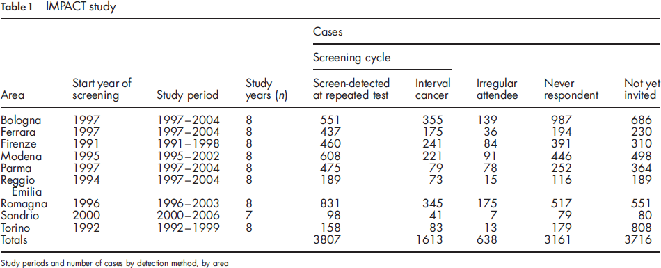
Figure 1 shows the O/E ratio (with 95% CIs) of invasive and in situ cases in the first eight years after screening start, which is near 1 in steady state.

Figure 1

IMPACT study. Observed/expected invasive and in situ cases by years of screening, with 95% CI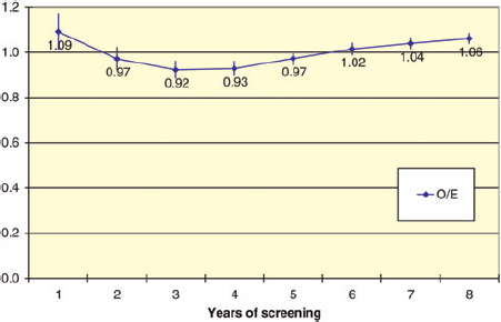

Table 2 shows the trend in cumulative episode sensitivity and annual programme sensitivity estimates from year 3 to year 8 of screening activity.

Table 2

IMPACT study

Years of screening	Episode cumulative sensitivity (95% CI)	Programme annual sensitivity (95% CI)
3	0.48 (0.43-0.53)	0.20 (0.18-0.23)
4	0.58 (0.54-0.62)	0.31 (0.28-0.34)
5	0.65 (0.62-0.68)	0.41 (0.38-0.44)
6	0.68 (0.66-0.71)	0.45 (0.42-0.48)
7	0.69(0.67-0.71)	0.42 (0.39-0.45)
8	0.70 (0.68-0.72)	0.48 (0.44-0.52)

Comparison of episode and programme sensitivity (with 95% CI), by years of screening

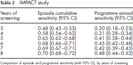
The programme sensitivity at steady state (from the fifth year of screening onward) ranged between 41% and 48% of the total number of cases in the target population.

Episode sensitivity progressively increased with time and reached a plateau of 0.70 at eight years after screening start. Sensitivity for invasive cases alone was slightly lower (0.68 - data not shown).

Episode sensitivity showed a clear trend across age groups, with lowest values in women aged 50-54 years (0.52 at year 8) and highest in those 65-69 (0.77) (Figure 2).

Figure 2

IMPACT study. Trends in episode cumulative sensitivity estimates from year 3 to year 8 of screening activity, by age class (invasive and in situ cases)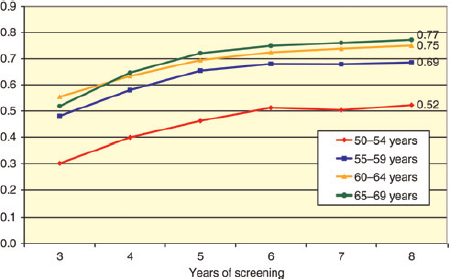

Discussion

We here present a method to estimate the sensitivity of screening programmes applied to a target screening population in steady state. This method represents a very serviceable tool to estimate the sensitivity of service screening programmes, because it does not depend on cohorts of screened women and hard-to-estimate data such as the underlying incidence trends (in the absence of screening).

The use of the steady state ratio screen-detected/(screen-detected + interval cases)¹¹ also largely overcomes the biases that affect the traditional method to calculate sensitivity. Slow-growing cancers (length bias), which would surface as symptomatic beyond the planned rescreening interval, or which would never become symptomatic during a lifetime (overdiagnosis), are likely to be included among cases screen-detected at prevalence screening, and so are excluded from this estimate. The results from the randomized clinical trials, reviewed by Sue Moss¹² in 2005, showed that in screening trials where the control group was screened at the end of the study period, the excess of incidence - and possible overdiagnosis - was practically absent.

Some of the assumptions of the model have been partially violated. Firstly, the model assumes a stable population in which the disease incidence rate and the screening intervals do not change with time or with the patient's age. However, in practice, incidence rates are increasing independently of the effect of service screening programmes. The yield of cases detected at a new screening round exceeds the expected number of cases, since the number of cases whose diagnosis is anticipated is greater than those stolen by the previous test. However, it is plausible that this only marginally affects the estimates. We carried out a sensitivity analysis including the 1.7% annual increase of breast cancer incidence in Italy⁸ and obtained a 0.5% decrease of the sensitivity estimate.

Additionally, because breast cancer incidence increases with age and SD_L cases are diagnosed at the end of the screening cycle, the sensitivity estimate will be artificially increased. It is plausible, though, that this effect is limited.

Secondly, the model assumes a fixed period of the screening cycle. However, there is a caveat, for if the period is much longer than two years, later screening will tend to resemble a prevalence screen and there will be an increase of the numerator in the sensitivity formula. The variation in screening interval within the IMPACT study data resulted in small effect in sensitivity. To estimate the episode sensitivity of a programme given the length of its period, we carried out a sensitivity analysis utilizing the IMPACT study database. We compared the observed sensitivity with that estimated by adding to the ICs the cases emerging at different intervals from the previous negative mammogram. When cases diagnosed up to 27 months were considered, sensitivity at year 8 after screening start was reduced by 2.4-0.68%. The sensitivity dropped by 3.7-0.67% when including cases diagnosed up to 30 months since negative screening. Of course this small effect is related to episodic variations in the interscreening interval, while systematic differences of the interval are expected to be adequately evidenced by the method.

Thirdly, the model assumes 100% compliance to later screening tests. If compliance is suboptimal, the number of detected SD_L cases will be lower than expected and, as a consequence, sensitivities will be underestimated. Under the assumption that the detection rates in women attending later screening tests and in non-attenders would be similar, we estimated the effect of non-attendance and reduction in sensitivity. A direct method to overcome this problem is to divide the SD by the estimate of attendance rate to second screen.

It should be pointed out that ICs diagnosed in women aged 70+ years must be excluded from the estimate, because they belong to an open-ended set, which is not closed with a subsequent screening test. Since sensitivity is greatest in the elderly, this leads to an underestimate of the overall sensitivity.

A proportion of ICs for some reason is not detected during the interval but is diagnosed at the subsequent screening episode. Our method does consider these cases as ‘successes’ and thus sensitivity is overestimated. To quantify this effect we reclassified the screen-detected cases that were pT3+ at diagnosis as interval cancers and observed a 4% reduction in sensitivity to 0.67 after eight years of screening.

It should also be recognized that the opposite may take place: some asymptomatic cancers are detected in women who spontaneously undergo a mammography during the interval. These cancers are labelled as failures (interval) instead of successes (detection at screening). The size of this effect is directly associated with the spread of interscreening examinations, that can be highly variable from place to place. In the IMPACT Study areas, we recoded the interval cases pTlb or less as screen-detected and obtained an 8.6% increase of sensitivity up to 0.76 at the eighth year of screening. This distortion clearly affects all methods to estimate sensitivity.

According to our estimates, the screening programmes included in the IMPACT study reported an overall sensitivity of 0.70 after eight years from screening start. This result is in accordance with the standard given in European Guidelines for interval cancer rate as a proportion of the background incidence rate (30% in the first 11 months of interval and 50% in months 12-23; onaverage,40%),¹³ and it is in agreement with many estimates in Italian programmes produced using the proportional incidence method,^{14

18} although not with all.¹⁹

Several papers have been published on sensitivity of breast cancer screening programmes in other countries, using both the proportional incidence method^{20

31} and other models.^{32

34} As shown in a recent paper by Törnberg et al.³⁵ who reported the results of programmes from six European countries, the comparison is very difficult because programmes have different characteristics (age group targeted, number of views, participation rates, etc.) that may deeply affect their sensitivity.

We observed a reduction in sensitivity with decreasing age as reported in many different studies.^17,36–42 This trend has been attributed mostly to the higher proportion of dense breasts in younger women.^43,44

In conclusion, the method produced reliable estimates of programme and episode sensitivity in steady state populations, i.e. when a service screening programme is mature after the first enrolment and prevalence screening period. The estimate is possible using cancer registry data and knowledge of diagnostic modality. Better knowledge of the contribution of the diagnostic true false-negative interval cancer cases in the estimate of sensitivity is possible if all breast cancer cases in the target population are classified by diagnostic modality in relation to screening.

IMPACT working group

E Paci, P Falini, D Puliti, I Esposito, M Zappa, E Crocetti (Clinical and Descriptive Epidemiology Unit - ISPO - Cancer Prevention and Research Institute, Firenze); S Ciatto (Department of Diagnostic Imaging - ISPO - Cancer Prevention and Research Institute, Firenze); C Naldoni, AC Finarelli, P Sassoli de Bianchi (Screening Programme, Department of Health, Regione Emilia-Romagna, Bologna); S Ferretti (Ferrara Cancer Registry, Dipartimento di Medicina Sperimentale e Diagnostica, Sezione di Anatomia, Istologia e Citologia Patologica, Università di Ferrara, Ferrara); GP Baraldi (Breast Cancer Screening Programme, Ferrara); M Federico, C Cirilli (Modena Cancer Registry, Modena); R Negri (AUSL, Modena); V De Lisi, P Sgargi (Parma Cancer Registry, Parma); A Traina, M Zarcone (Department of Oncology, ARNAS Ascoli, Palermo); A Cattani, N Borciani (AUSL, Reggio Emilia); L Mangone (Registro Tumori di Reggio Emilia, Dipartimento di Sanità Pubblica, AUSL, Reggio Emilia); F Falcini, A Ravaioli, R Vattiato, A Colamartini (Romagna Cancer Registry, IRST, Forli); M Serafini, B Vitali, P Bravetti (AUSL, Ravenna); F Desiderio, D Canuti, C Fabbri (AUSL, Rimini); A Bondi, C Imolesi (AUSL, Cesena); N Collina, P Baldazzi, M Manfredi, V Perlangeli, C Petrucci, G Saguatti (AUSL, Bologna); N Segnan, A Ponti, G Del Mastro, C Senore, A Frigerio, S Pitarella (CPO Piemonte, AO San Giovanni Battista, Torino); S Patriarca, R Zanetti (Registro Tumori Piemonte, CPO Piemonte, AO San Giovanni Battista, Torino); M Vettorazzi, M Zorzi (Venetian Tumour Registry, Istituto Oncologico Veneto - IOV IRCCS, Padova); A Molino, A Mercanti (Università di Verona, Verona); F Caumo (Azienda ULSS, Verona); R Tumino, A Sigona (Registro Tumori, UO Anatomia Patologica, Azienda Ospedaliera Civile MP Arezzo, Ragusa); G La Perna, C Iacono, ONCOIBLA e UO di Oncologia, AO Ragusa, Ragusa); F Stracci, F La Rosa (Registro Tumori Umbro, Perugia); M Petrella, I FuscoMoffa (Epidemiology Unit, ASL2, Perugia).

Contributors: MZ and EP designed the study and drafted the manuscript. SG did the statistical analyses. MZ and SG prepared the figures and tables. DP collected the data. All authors critically reviewed the manuscript and approved the final version. EP is the guarantor.

Footnotes

None declared. This study was supported in part by research grants from the Italian Ministry of Health, Regione Abruzzo, and the Italian League against Cancer, Rome. The sponsors had no role in the collection, analysis and interpretation of data, in the writing of this report, and in the decision to submit the manuscript for publication.

Acknowledgment

Thanks to Nigel Barton for the English revision of the draft.

Graphical Demonstration of the Principle of the Steady-State Behaviour of a Screening Programme

Consider a population of n women at a single moment of time. Breast cancers in a preclinical phase will be present and unknown (shaded area in Figure A1). These cancers are at different states of development or growth - some being very immature, and others very mature. We can imagine the cancers arrayed as in Figure A1 according to their states. If the subgroup of women affected by a cancer simultaneously undergoes a diagnostic test (e.g. a mammogram), the probability that the test will be positive depends on the state of development of that cancer.

Figure A1-A8

Principle of the steady-state behaviour. Graphical demonstration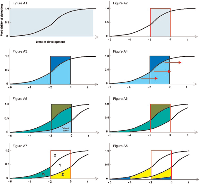

It is reasonable to assume that the more mature the cancer, the higher the probability. In other words, this probability is a function of the state of development of the cancer and is represented in Figure A1 by the black curve (the ‘detection probability curve’). Now let us put the state of development on a timescale and pick an arbitrary reference point in the life of the lesion (t = 0) corresponding to the moment of incidence, defined as the moment the patient would seek care on her own, and draw the timescale before that point (Figure A2).

Let the annual incidence rate of cancers be R per n women years: in our population there are R whose cancers are in a development state between -1 and 0, and R more with cancers in states between -2 and -1, and so forth. In the absence of screening, the cancers that will be diagnosed in the following two years are those whose state is between -2 and 0 (shaded area in Figure A2).

Suppose that we screen these women with a mammogram and let the screening interval be two years. The light blue area under the detection probability curve in Figure A3 represents the number of cases we expect to detect. Screening is imperfect, so there are a number of cancers that are not picked up by mammography, but that will come to clinical attention in the following two years (the dark blue area in Figure A3). They are the interval cancers of the first screening round.

At the time of the first re-examination two years have passed and all of the women in Figure A3 have moved along the horizontal axis two units to the right (Figure A4). The results of the second mammogram are different, because some of the cancers in this population have already been diagnosed by the previous screening episode (labelled as ‘stolen’ in Figure A5). The light green area in Figure A5 represents the cases screen-detected at the second episode. The dark green area represents the interval cases of the second screening round.

We want now to show that the periodic yield of cancers detected by all methods after the initial examination is approximately equal to the biennial incidence rate. We can achieve this by showing that the sum of the areas in Figure A6 shaded light and dark green (respectively, cancers detected in the first re-examination and in the interval) equals the area inside the red rectangle based on the interval - 2 to 0, which is the biennial incidence rate. As the two areas labelled as X and Y are common (Figure A7), and the equivalence of those labelled Z and W is shown in Figure A8 (where the two yellow areas are equal, and, so too, are the violet areas) the demonstration is complete.

References

Hakama

, Auvinen

, Day

, Miller

. Sensitivity in cancer screening. J Med Screen 2007; 14: 174–7

Day

, Williams

, Khaw

. Breast cancer screening programmes: the development of a monitoring and evaluation system. Br J Cancer 1989; 59: 954–8

Cuzick

, Edwards

, Segnan

. Adjusting for non-compliance and contamination in randomized clinical trials. Stat Med 1997; 16: 1017–29

Ciatto

, Naldoni

, Ponti

. Interval cancers as indicators of performance in screening programmes. Epidemiol Prev 2008; 32: 93–8

Eddy

. Screening for Cancer. Theory, Analysis and Design. Englewood Cliffs, NJ: Prentice-Hall, 1980

Baker

, Kramer

, Prorok

. Comparing breast cancer mortality rates before-and-after a change in availability of screening in different regions: extension of the paired availability design. BMC Med Res Methodol 2004; 18: 12

Giordano

, Giorgi

, Fasolo

, Segnan

, Del Turco

. Breast cancer screening: characteristics and results of the Italian programmes in the Italian group for planning and evaluating breast cancer screening programmes (GISMa). Tumori 1996; 82: 31–7

AIRTum Working Group.

I tumori in Italia - Rapporto 2006. Incidenza, mortalità e stime.

Epidemiol Prev 2006: 30(Suppl. 2):36–41

Paci

, Miccinesi

, Puliti

. Estimate of overdiagnosis of breast cancer due to mammography after adjustment for lead time. A service screening study in Italy. Breast Cancer Res 2006; 8: pR68

10.

Breslow

, Day

. Statistical Methods in Cancer Research, Vol. 2 - The Design and Analysis of Cohort Studies. New York: Oxford University Press, International Agency for Research on Cancer, 1989

11.

Shapiro

. Evidence on screening for breast cancer from a randomized trial. In: Strax

, ed. Control of Breast Cancer through Mass Screening. Littleton, MA: PSG Publishing, 1979: 19–36

12.

Moss

. Overdiagnosis and overtreatment of breast cancer: overdiagnosis in randomised controlled trials of breast cancer screening. Breast Cancer Res 2005; 7: 230–4

13.

Perry

, Broeders

, de Wolf

. European Guidelines for Quality Assurance in Breast Cancer Screening and Diagnosis. 4th edn. Luxembourg: European Commission, 2006

14.

Burani

, Caimi

, Maggioni

. Quality assessment of the mammographic screening programme in the Azienda Sanitaria locale Provincia Milano 1 - analysis of interval cancers and discussion of possible causes of diagnostic error. Radiol Med 2005; 109: 260–7

15.

Giorgi Rossi

, Federici

, Farchi

. The effect of screening programmes on the treatment of benign breast neoplasms: observations from current practice in Italy. J Med Screen 2006; 13: 123–8

16.

Vettorazzi

, Stocco

, Chirico

. Quality control of mammography screening in the Veneto Region. Evaluation of four programmes at a Local Health Unit level - analysis of the frequency and diagnostic pattern of interval cancers. Tumori 2006; 92: 1–5

17.

Paci

, Ciatto

, Buiatti

, Cecchini

. Early indicators of efficacy of breast screening programmes. Results of the Florence District Programme. Int J Cancer 1990; 46: 198–202

18.

Törnberg

, Codd

, Rodrigues

, Segnan

, Ponti

. Ascertainment and evaluation of interval cancers in population-based mammography screening programmes: a collaborative study in four European centres. J Med Screen 2005; 12: 43–9

19.

Zappa

, Falini

, Bonardi

. Monitoring interval cancers in mammographic screening: the Florence District Programme experience. Breast 2002; 11: 301–5

20.

Asbury

, Boggis

, Sheals

, Threlfall

, Woodman

. NHS breast screening programme: is the high incidence of interval cancers inevitable? BMJ 1996; 313: 1369–70

21.

Blanks

, Moss

. Monitoring the performance of breast screening programmes: allowing for geographical variation in breast cancer incidence. J Med Screen 1996; 3: 82–4

22.

Faux

, Richardson

, Lawrence

, Wheaton

, Wallis

. Interval breast cancers in the NHS breast screening programme: does the current definition exclude too many? J Med Screen 1997; 4: 169–73

23.

Fracheboud

, de Koning

, Beemsterboer

. Interval cancers in the Dutch breast cancer screening programme. Br J Cancer 1999; 81: 912–17

24.

Everington

, Gilbert

, Tyack

, Warner

. The Scottish breast screening programme's experience of monitoring interval cancers. J Med Screen 1999; 6: 21–7

25.

Exbrayat

, Garnier

, Colonna

. Analysis and classification of interval cancers in a French breast cancer screening programme (department of Isere). Eur J Cancer Prev 1999; 8: 255–60

26.

Kavanagh

, Mitchell

, Farrugia

, Giles

GG.

Monitoring interval cancers in an Australian mammographic screening programme.

J Med Screen 1999; 6: 139–43

27.

Hofvind

, Bjurstam

, Sorum

, Bjorndal

, Thoresen

, Skaane

. Number and characteristics of breast cancer cases diagnosed in four periods in the screening interval of a biennial population-based screening programme. J Med Screen 2006; 13: 192–6

28.

Lynge

. Mammography screening for breast cancer in Copenhagen April 1991-March 1997. Mammography Screening Evaluation Group. APMIS Suppl 1998; 83: 1–44W

29.

Johnson

, Shekhdar

. Interval cancers in the National Health Service Breast Screening Programme. Br J Radiol 1995; 68: 862–9

30.

Day

, McCann

, Camilleri-Ferrante

. Monitoring interval cancers in breast screening programmes: the East Anglian experience. Quality Assurance Management Group of the East Anglian Breast Screening Programme. J Med Screen 1995; 2: 180–5

31.

Sylvester

, Vipond

, Kutt

, Davies

, Webb

, Farndon

. A comparative audit of prevalent, incident and interval cancers in the Avon breast screening programme. Ann R Coll Surg Engl 1997; 79: 272–5

32.

Shen

, Zelen

. Parametric estimation procedures for screening programmes: stable and nonstable disease models for multimodality case finding. Biometrika 1999; 86: 503–15

33.

Shen

, Zelen

. Screening sensitivity and sojourn time from breast cancer early detection clinical trials: mammograms and physical examinations. J Clin Oncol 2001; 19: 3490–9

34.

Straatman

, Peer

, Verbeek

. Estimating lead time and sensitivity in a screening program without estimating the incidence in the screened group. Biometrics 1997; 53: 217–29

35.

Törnberg

, Kemetli

, Ascunce

. A pooled analysis of interval cancer rates in six European countries. Eur J Cancer Prev 2010; 19: 87–93

36.

Sarkeala

, Hakama

, Saarenmaa

, Hakulinen

, Forsman

, Anttila

. Episode sensitivity in association with process indicators in the Finnish breast cancer screening program. Int J Cancer 2006; 118: 174–9

37.

Tabar

, Faberberg

, Day

, Holmberg

. What is the optimum interval between mammographic screening examinations? An analysis based on the latest results of the Swedish two-county breast cancer screening trial. Br J Cancer 1987; 55: 547–51

38.

Taylor

, Supramaniam

, Rickard

, Estoesta

, Moreira

. Interval breast cancers in New South Wales, Australia, and comparisons with trials and other mammographic screening programmes. J Med Screen 2002; 9: 20–5

39.

Ciatto

, Visioli

, Paci

, Zappa

. Breast density as a determinant of interval cancer at mammographic screening. Br J Cancer 2004; 90: 393–6

40.

Hofvind

, Wang

, Thoresen

. Do the results of the process indicators in the Norwegian breast cancer screening program predict future mortality reduction from breast cancer? Acta Oncol 2004; 5: 467–73

41.

Kavanagh

, Mitchell

, Farrugia

, Giles

. Monitoring interval cancers in an Australian mammographic screening programme. J Med Screen 1999; 6: 139–43

42.

Rickard

, Taylor

, Fazli

, El Hassan

. Interval breast cancers in an Australian mammographic screening program. Med J Aust 1998; 169: 184–7

43.

Buist

, Porter

, Lehman

, Taplin

, White

. Factors contributing to mammography failure in women aged 40-49 years. J Natl Cancer Inst 2004; 96: 1432–40

44.

Carney

, Miglioretti

, Yankaskas

. Individual and combined effects of age, breast density, and hormone replacement therapy use on the accuracy of screening mammography. Ann Intern Med 2003; 138: 168–75

A simple method to estimate the episode and programme sensitivity of breast cancer screening programmes

Abstract

Background

Methods

Results

Conclusions

Introduction

Methods

Application to the IMPACT Study data

Results

Discussion

IMPACT working group

Footnotes

Acknowledgment

Graphical Demonstration of the Principle of the Steady-State Behaviour of a Screening Programme

References