
Abstract
Objectives
Data on the performance of health boards, hospitals and medical specialists, etc., are being collected at various levels in the health-care system and are often presented as league tables. These tables ignore natural variation and/or confounders, and this introduces uncertainty about their interpretation. The purpose of this study was to devise and illustrate a method to expose the real difference between the ratings in league tables.
Methods
Two values per rating were added to the league tables: the best-case scenario and the worst-case scenario. True performance will lie somewhere between these two values. The method is illustrated using data from the Dutch breast cancer screening programme.
Results
By focusing on one performance indicator and one confounder, it was possible to show shifts in the rating order of breast cancer screening units and thus expose the uncertainty about the true performance of each screening unit.
Conclusions
The worst-case and best-case scenario ratings demonstrated the uncertainty within the ratings of a league table. League tables should therefore only be used with great caution and after providing the public with sufficient information.
Introduction
There is great concern about the manner in which the data are being presented and interpreted. In particular, a large difference in rank may reflect only trivial (i.e. not clinically meaningful) differences in actual outcome. 3
A major disadvantage of presenting ratings alone is that valuable information is lost. It is impossible to see whether the difference in performance between two institutions with similar ratings is large or meaningless. When data are presented in the form of means, rates, odds ratios, etc., it is common to see a confidence interval, which is rarely the case with league tables. Therefore, league tables should be accompanied by an indication of their precision if they are to be of any help to patients, care providers, purchasers of care, or the government.
League tables are often used when an outcome measure is expressed as a total score. For example, the magazine U.S. News used a total score to compile a league table of American cancer hospitals. 4 Their total score was calculated from nine subscores that varied from reputation (in %), number of discharges and being an NCI cancer centre (yes/no). A difference of, for example, five points on this scale is impossible to interpret, so the scores were put into league tables. Confounding variables were ignored. A method is needed to expose the uncertainty within the rating of each individual institution.
In essence, differences in performance are caused by three factors:
Quality, i.e. technical expertise and equipment, organizational aspects, quality indicators for the care or service delivered;
Confounders, such as patient case mix;
Natural variation.
If natural variation and confounders are filtered out, the real differences in performance will become apparent, instead of the observed differences. It is necessary to adjust for the confounders and such an adjustment can have a heavy impact on the league table. Natural variation is present in all data. These fluctuations in results are caused by chance variability and they increase as the number of observations decreases. Therefore, smaller institutions are more likely to show over-performance or under-performance than larger ones, even if this is not true.
This article explains how to expose the magnitude of the influence of natural variation on the league table, after adjustment for confounding variables. The method introduces the best-case scenario and the worst-case scenario into the rating, and is illustrated using data from 18 central screening units in the Dutch breast cancer screening programme. First, the best-case scenario and the worst-case scenario ratings at each central screening unit were calculated, then the calculation was repeated while adjusting for the age of the women.
Marshall and Spiegelhalter 5 used another method to show the variability of the rankings, based on constructing credible intervals for the rankings. The results of the two methods are compared.
Presentation of the best-case scenario, the worst-case scenario and the adjusted rating will illustrate clearly the magnitude of the influence of natural variation on the league table. Patients and insurance companies can understand that the true rating may be as good as the best-case scenario, while the central screening unit can view the worst-case scenario as a warning: if no action is taken, next years’ rating may drop to this level.
Patients and Methods
Patients
The Dutch screening programme for breast cancer was gradually implemented over the period 1988–1997. Its main characteristics are the centralized organization (including centralized technical and medical quality control and audit), the two-year interval between screening examinations and the eligible age of 50–74 years. Technical and medical quality control are the responsibility of the National Expert and Training Centre. Data collection, evaluation and annual reporting of the results are performed by the National Evaluation Team. 6 In 2004 and in 2005, annually almost 1.1 million women aged 50–74 years were invited for a screening examination. Participation was 81% and breast cancer was detected in approximately 5%o of the invited women. 7 It has been estimated that the national breast cancer screening programme reduces the number of women who die from breast cancer by 700 per year. 8 In 2005, breast cancer mortality in women aged 55–74 years was 26% lower than in 1986–1988, i.e. before the start of the programme. 7
The Dutch screening programme has a central organization that oversees nine screening regions. Each region has 1–5 central screening units. Radiologists evaluate the screening radiographs. Site visits to the central screening units are performed once every three years by the National Reference Centre. They monitor the performance of the radiologists and radiographers and check the technical and positioning quality of the mammograms. In addition, they review data from two screening rounds and a selection of cancer cases. 6 The site visit report contains data on performance indicators, such as number of women screened, age, referral rate, detection rate and tumour stage distributions. Some of these data were used as a model in the present study.
In our analysis, we drew data on detection rates and age from the 18 central screening units that were visited in the period 2003–2005. We selected only women who had been screened at least once before. The women were divided into two age groups: 49–69 years and 70–74 years.
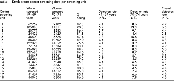
The raw data from each central screening unit are presented in Table 1: the number of women screened in the two age groups, the percentage of women in the younger age group, the detection rates in the two age groups and the overall detection rates.
Dutch breast cancer screening data per screening unit
Methods
The first part of this section explains the general method when the outcome variable has not been adjusted for confounding variables. This method has been previously explained in Lemmers et al., 9 but has nevertheless been repeated for the convenience of the reader. Furthermore, it makes the new part, how to adjust the outcome variable for confounding variables, easier to comprehend. Calculations are shown for the rating, the best-case scenario and the worst-case scenario for the rating. The second part illustrates how these values can be calculated after the outcome variable has been adjusted for confounders.
(A) When the outcome variable has not been adjusted
To calculate the rating, the best-case scenario and the worst-case scenario for the rating of a screening unit (a clinic or a medical specialist), the following is needed:
Estimates of the performance of the screening unit compared with each of the other screening units (e.g. an odds ratio, or a difference between means);
Reasonable estimates of the lower bound of the performance (e.g. the lower bound of a 95% confidence interval in the case of an odds ratio, or the lower bound of a 95% confidence interval in the case of a difference between means);
Reasonable estimates of the upper bound of the performance (e.g. the upper bound of a 95% confidence interval in the case of an odds ratio, or the upper bound of a 95% confidence interval in the case of a difference between means).
If, for example, the upper bound of the 95% confidence interval of the odds ratio for detection at a particular screening unit versus another screening unit is larger than one, we interpret this as ‘When the first screening unit has the benefit of the doubt compared with the second screening unit, it is more likely that breast cancer will be detected in the first screening unit than in the second screening unit’. We then say that in the best-case scenario the performance of the first screening unit is better than that of the second screening unit.
Similarly, if the lower bound of the 95% confidence interval of the odds ratio for detection at a particular screening unit versus another screening unit is larger than one, we interpret this as ‘When the first screening unit has everything going against it compared with the second screening unit, it is still more likely that breast cancer will be detected at the first screening unit than at the second screening unit’. We then say that in the worst-case scenario the performance of the first screening unit is better than that of the second screening unit.
We performed a logistic regression analysis on the detection rate as outcome variable with one covariate, namely screening unit (as a class variable). We obtained from each screening unit the odds ratios for detection of cancer at this unit versus detection at each of the other screening units, with corresponding 95% confidence intervals. As relatively few of the women received a screen-positive result (around 5%o), these odds ratios can be interpreted as relative risks.
Next, we calculated the unadjusted rating, the best-case scenario and the worst-case scenario for the rating of each screening unit. The unadjusted rating of the first screening unit was 1+ the number of screening units whose performance was better than that at screening unit 1. The best-case scenario for the rating of the first screening unit was 1+ the number of screening units whose performance was better than that at screening unit 1, even when screening unit 1 was given the benefit of the doubt. This was 1+ the number of screening units for which the 95% upper bound of the odds ratio for detection at screening unit 1 versus detection at this particular screening unit was smaller than 1. Similarly, the worst-case scenario for the rating of the first screening unit was 1+ the number of screening units whose performance was better than that at screening unit 1 when everything was going against screening unit 1. This was 1+ the number of screening units for which the 95% lower bound of the odds ratio for detection at screening unit 1 versus detection at this particular screening unit was smaller than 1.
(B) When the outcome variable has been adjusted
When the outcome variable has been adjusted for one or more confounders, estimates of the differences in performance are used after adjustment for confounding covariates. A continuous outcome variable, such as length of hospitalization, can be adjusted using linear regression. A dichotomous outcome variable can be adjusted using logistic regression, as we show below using the same breast cancer screening data as before.
We performed a logistic regression analysis on the outcome variable breast cancer detection rate, with two covariates, namely age group and screening unit (as class variables). We obtained from every screening unit the odds ratio for detection of cancer at this unit versus detection at each other screening unit, adjusted for age, with corresponding 95% confidence intervals. Then, using the same method as in the previous section, we calculated the rating, the best-case scenario and the worst-case scenario of each screening unit, based on the odds ratios for breast cancer detection adjusted for age.
Results
Table 2 summarizes the results at each screening unit. Except for screening units 4, 7 and 12, all the screening units had a best-case scenario of 1, 2 or 3 before adjustment for age. After adjustment, the ratings of 10 out of the 18 central screening units deviated by a maximum of two positions. The screening units with different ratings after adjustment are shown in bold-type. Even after adjustment, except for screening units 4, 7 and 12, all the screening units had a best-case scenario rating of 1, 2 or 3.
Dutch breast cancer screening unit league table, with rating, best-case scenario and worst-case scenario ratings, before and after adjustment for age
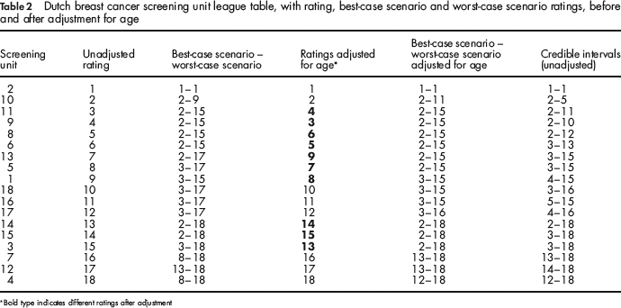
Bold type indicates different ratings after adjustment
Figure 1 shows the adjusted rating and the range from the best-case scenario to the worst-case scenario of each screening unit. The lower endpoint of a vertical line represents the best-case scenario, while the upper endpoint indicates the worst-case scenario of the unadjusted rating. The adjusted rating is indicated with a horizontal line.
Graphic representation of the performance of 18 Dutch breast cancer screening units according to their detection rate adjusted for age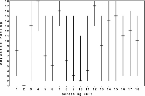
Comparison with the credible interval method
In this section, we compare the results of our method with the credible interval method. This method was used by Marshall and Spiegelhalter, 5 who studied the reliability of league tables of IVF clinics. When the credible interval method is used, bootstrap samples are drawn and the resulting replications are analysed. The results of the comparison are shown in the sixth column of Table 2.
The credible intervals are in general somewhat narrower than the best-case worst-case intervals. To understand why this is the case, we consider an example in which all units have the same size. Suppose that the lower limit of the 95% confidence interval of the difference between the best scoring unit B and another unit U is just below zero. Then the best-case scenario of unit U is 1. If there are only two units, unit U is then expected to have ranking 1 in just over 2.5% of the replicates, so the upper limit of the credibility interval for U is 1. However, when there are more units, this may reduce the number of times that U has score 1 to less than 2.5%. As a consequence, the upper limit of the credibility interval for the ranking of unit U will not be 1, but the upper limit of the best-case worst-case interval will be.
Discussion
In a league table, it is impossible to perceive whether there is any real difference between the ratings. Differences in rating between e.g. two institutions, centres or units, might be caused by confounding variables and/or by natural variation. Adding the best-case and worst-case scenarios to the adjusted rating will show the magnitude of the influence of natural variation on the league table, while adjusting for confounders. This puts the values and positions in better perspective, because we can see whether there is any real difference. We saw that there were sometimes large differences in best-case scenarios and worst-case scenarios between the screening units in the league table, which meant that there was great uncertainty about the true position of each particular screening unit.
The best-case scenario rating of a screening unit indicates the position that a screening unit would take in the league table if it had everything going for it. The worst-case scenario rating indicates the position that a screening unit would take if it had everything going against it. Thus, the true rating of a screening unit can be expected to lie somewhere between the best-case scenario and the worst-case scenario.
Besides natural variation, another well-known cause of the differences in performance is confounding. In the example, adjustment was made for age, but several other factors can influence the results and differ between screening units. We only adjusted for age and not for other factors, because we wanted to give a clear illustration of our method. Extra adjustments would probably influence the ratings. Table 2 shows for example that there were differences between the league tables before and after adjustment: screening unit 3 climbed 2 places after adjustment.
The selection of data from the breast cancer screening programme over-simplified the comparison between screening units. Performance is not only determined by detection rates, but also by indicators, such as:
the percentage of women in the screening population who are screened at the unit;
the percentage of women who are referred for further tests and are diagnosed with breast cancer;
the size and stage of the cancers of the screen-detected breast malignancies: e.g. the performance of a screening unit that detects mostly small malignancies is better than that of a screening unit that detects mostly large malignancies when they have the same detection rate;
the number of women diagnosed with interval cancer;
and several other factors.
These performance indicators are known to vary between screening units. Typically, however, there is no consistent pattern in which one unit outperforms the others on all the indicators. In addition, the number of screen-positive women should be weighed against the number of women who are referred for further tests but do not have breast cancer (false-positive) and the number of women diagnosed with interval breast cancer (false-negative). A review study by Otten et al. on interval and screen-detected breast malignancies showed a delicate balance between recall, detection and false-positive rates. 10
A reliable total score that gives a good reflection of the performance of a screening unit consists of a combination of several scores on each part of the chain of care, e.g. scores on the radiologist, the technical quality of the mammograms and the level of compliance with guidelines. This total score should be adjusted for some factors, such as the time period reporting took place. Interpretation of total scores (and their confidence intervals) is notoriously difficult, because what does a difference of 5 points mean in practice? Thus, the only option is to resort to a league table anyway. If the best-case scenario and worst-case scenario are also presented, then the range of statistical dispersion will be easier to interpret.
There are several alternatives to our method. A more conservative or less conservative method can be chosen depending on the situation. If the goal is to expose even relatively small differences in the league, even at the cost of some additional false alarms, the credible interval method 5 should be used, or our method with, e.g., 90% confidence intervals. If the goal is to prevent premature action, our method could be used with Bonferroni correction to correct for the multiple comparisons that are being made, or with wide confidence intervals (e.g. 99%).
Confidence intervals can also be presented with the (adjusted) detection rate at each screening unit. This has the advantage that the differences in performance become visible, which provides more scope than ratings alone. However, there is sometimes more interest in the league table than in any differences. Therefore, it is necessary to develop methods that give an accurate portrayal of the spread and spacing of ratings. The results of these methods should be easy to interpret, so that non-statisticians also have access to adequate information.
Conclusions
The method illustrated here is easy to implement and the results are easy to interpret. By adding a best-case scenario and a worst-case scenario, the screening units were rated according to their performance, without doing them any injustice, because natural variation and confounders were incorporated into these additional ratings. If the differences are real, even after adjustment, our method distinguishes between screening units whose performance is significantly poorer (or better). If natural variation is the only cause of the observed differences, our method prevents any premature judgement and thus avoids unnecessary anxiety, stigma and guilt. These are important improvements, for patients, care providers and purchasers of health care.