
Abstract
Transformations from austenite to martensite or bainite in ferrous alloys have great technological importance, but some aspects remain elusive. The orientation relationship (OR), morphology and habit plane can vary considerably from one system to another. Much published work considers these OR in terms of their variation from named relationships such as Kurdjumov–Sachs and Nishiyama–Wassermann. We discuss here, instead, the use of a set of angular parameters based on the classic work of Kurdjumov and Sachs in the 1930s, that provide a unified and elegant description facilitating extraction and detailed statistical treatment of OR from large electron backscatter diffraction datasets, as well as straightforward comparison with named OR and with the predictions from the phenomenological theory. Spatially correlated mappings of OR parameters obtained using this approach suggest that the observed variations in OR are related to the martensitic morphology rather than being an experimental artefact.
Keywords
Introduction
The diffusionless transformation from austenite (γ) to martensite (α′) occurs according to a fixed crystallographic orientation relationship (OR). As a result of crystal symmetry, up to 24 orientational variants may satisfy the OR, and a single austenite grain generally subdivides into numerous crystallites, each exhibiting one of the variants. Orientation relationships of this type are also observed in bainitic and Widmannstätten ferrite. Two famous orientation relationships, determined using X-ray diffraction in the 1930s, are the Kurdjumov–Sachs (KS) OR identified in a mild steel
1


As the use of electron backscatter diffraction (EBSD) has become more widespread, it has also become apparent that there is considerable variation in the orientation relationships observed from a single sample.10–12 It is as yet unclear whether this variation is an artefact of the small sizes of the crystallites involved, as suggested by Bhadeshia, 20 or whether it has some relationship to the transformation mechanism, arising, for example, from the high dislocation density induced during the transformation or from local modifications in the orientation of the parent austenite as a result of transformation strain. Statistical distributions and spatially correlated plots of parameters characterising the OR could help to elucidate this.
Possible parametric representations of orientation relationships include orientation matrices or Euler angles. However, the former contain redundant information, and both representations suffer from the need to select both a representative variant from a possible 24, and a representative choice from the set of symmetrically equivalent ways to express this orientation, in order to reduce the dataset such that it can be analysed statistically. The present paper discusses an approach based on a section in the classic work by Kurdjumov and Sachs that has thus far received comparatively little attention.
Methods
Definition of parameters
In their paper of 1930, Kurdjumov and Sachs describe the orientation relationship between austenite and martensite not only in terms of the well-known parallelism reproduced above, but also in terms of small angular deviations between planes in the martensitic unit cell and nearby planes in the austenite (Ref. 1, Table 1). The planes listed for the martensite represent the faces of the body-centred tetragonal (bct) or cubic (bcc) unit cell, while the planes listed for the austenite correspond to the faces of one of the alternative bct ‘Bain’ unit cells that can be drawn in the face-centred cubic (fcc) austenite. 21 Although Kurdjumov and Sachs did not discuss them in great detail, these three angles, called ξ1, ξ2 and ξ3 in the present work, together characterise the rigid-body rotation (RBR) needed to bring the Bain cell into coincidence with the martensite unit cell. (More precisely, the cosines of these three angles are the diagonal elements of the RBR matrix, and the other elements can be determined from these.) Advantages of this notation are:
Definitions of Kurdjumov–Sachs angles ξ1, ξ2 and ξ3 with values measured by Kurdjumov and Sachs 1 and values for ideal KS and NW relationships assuming cubic product phase α
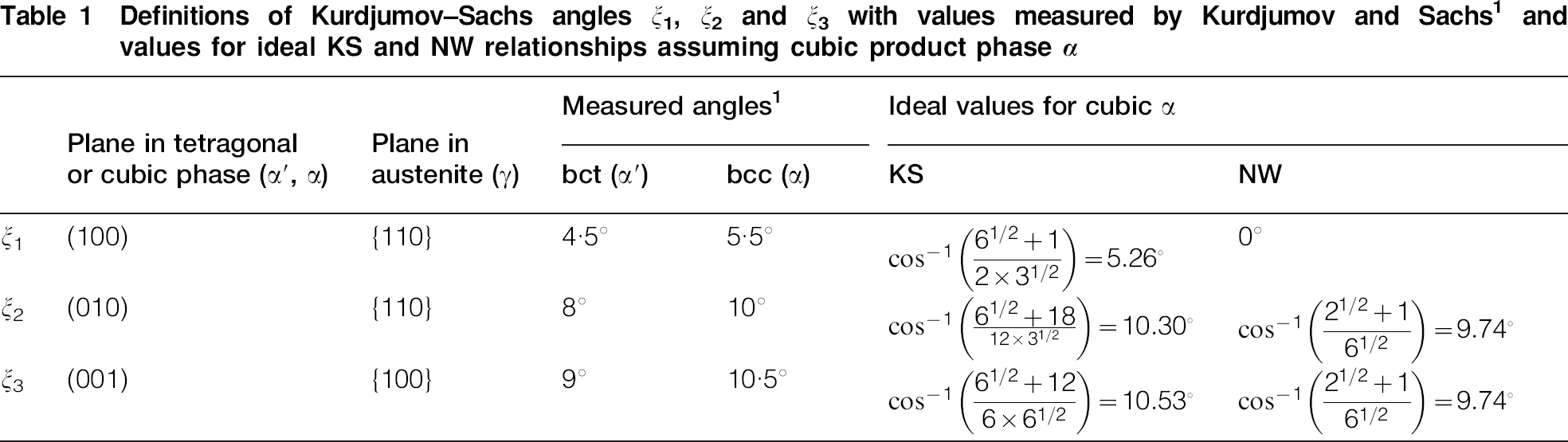
it separates out the symmetry-related part of the transformation (the symmetrically related Bain unit cells) from the material-specific part (the three angles, which relate each variant to its nearest Bain cell), avoiding complications involving the choice of a single ‘representative variant’
it allows ready comparison between ideal plane-parallel OR (see the exact and approximate values for KS and NW given in Table 1), predicted OR from the phenomenological theory and experimentally determined OR
the parameters can be extracted rapidly from experimental EBSD datasets. Their statistical distributions, or distributions of parameters derived from them (for example the Euler angles corresponding to the RBR) can then be analysed.
Extraction of parameters from EBSD datasets
Electron backscatter diffraction orientation data from commercial software are typically in the form of a set of Euler angles for each (x, y) position on the sample surface. In general, the dataset will consist of information from a number of different prior austenite grains, each of which may be oriented arbitrarily with respect to the polished surface. A single orientation may be represented by one of a number of symmetrically equivalent sets of Euler angles. A number of processing steps are therefore required in order to extract orientation relationship parameters from EBSD data. The procedure may in principle be employed to analyse orientation relationship data obtained with any set of microscope and/or EBSD collection parameters reasonable for microstructural mapping, although for statistical analysis, larger datasets are clearly preferable:
selection of a prior austenite grain: this can be done using the ‘highlighting’ functionality of commercial EBSD analysis software or by selection of a region of the image. The pole figure from the selected data should be checked to ensure that the data come from a single prior austenite grain with no twins. (If the data come from a single prior austenite grain, it should be possible to rotate the dataset such that the appearance of the {001} pole figure is similar to those shown in Fig. 1.) Points of low orientation confidence should be excluded from the dataset in this step
determination of the parent austenite orientation and rotation of the martensite dataset such that the parent austenite orientation comes into coincidence with the sample coordinate system. When no retained austenite is present, this rotation can be performed either by eye, which is generally sufficient, or using an automated procedure in which an initial guess of the orientation relationship between the parent and product phases (such as KS, GT, or NW) is taken, the estimated set of possible prior austenite orientations is calculated based on this guess, the modal value of these possible orientations is found, and then the reverse of the estimated probable prior austenite orientation is applied to the martensite dataset. If retained austenite is present, this can be used to perform the rotation, although it must be borne in mind that the martensitic transformation can induce strains in the parent austenite such that the measured orientation of small amounts of retained austenite may not be exactly equal to that of the original parent
transformation to matrix notation
determination of nearest Bain unit cell orientation and rotation by its inverse to obtain the RBR matrix16–18
determination of the diagonal elements of this and their inverse cosines; identification of ξ1, ξ2 and ξ3 based on the fact that ξ3 is the angle between (001)α’ and {100}γ, and ξ1<ξ2.
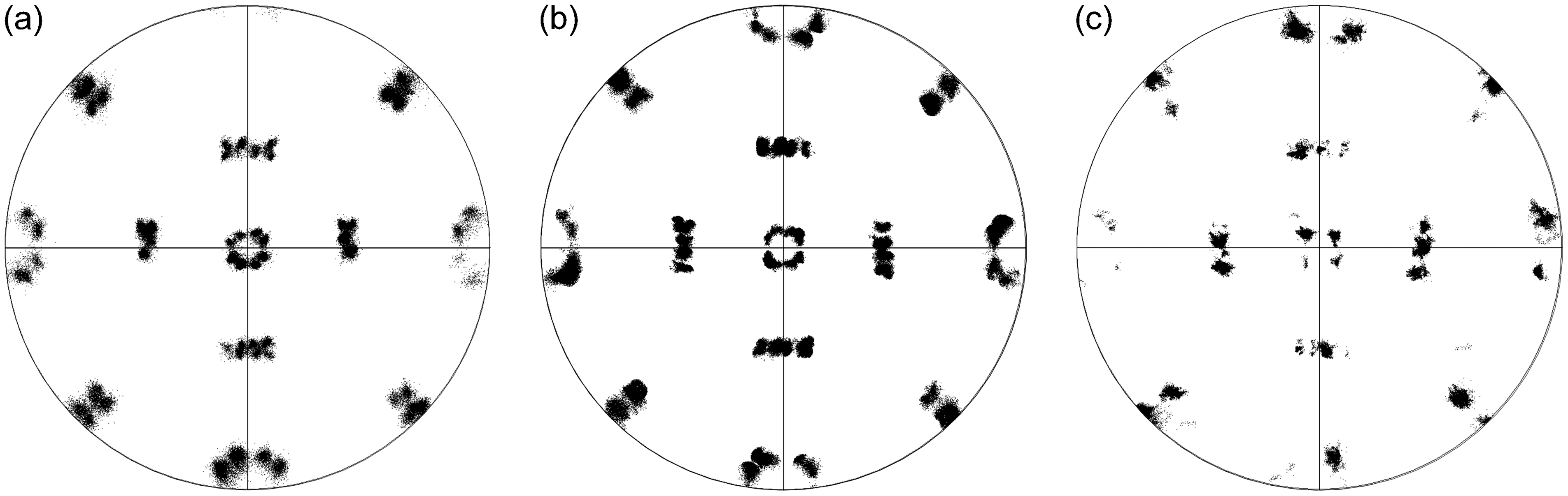
{001}α’ pole figures from single prior austenite grains of a low-carbon steel, b FV535 tempered martensitic steel and c Fe–30 at-Ni alloy
A program to automate the above procedure and to analyse the output has been written using the Matlab orientation and texture analysis toolbox MTEX. 22
Acquisition and processing of example datasets
Three example datasets have been chosen for analysis, based on the differences in their {001} pole figures, as discussed in the section on ‘OR differences between different materials’ below. The first of these comes from a low-carbon steel; the composition, thermal history and data acquisition parameters for this sample are reported in Ref. 23. The second and third datasets, from the tempered martensitic heat-resistant steel FV535 (German grade X8CrCoNiMo11) and an Fe–30 at-Ni binary alloy respectively, were acquired using standard metallographic preparation followed by surface treatment with colloidal silica suspension in a Vibromet automatic polisher (Struers GmbH, Willich, Germany). Data were acquired using a LEO1530VP field emission scanning electron microscope (Carl Zeiss NTS GmbH, Oberkochen, Germany) equipped with a Digiview camera and TSL software (EDAX, Mahwah, NJ, USA). The accelerating voltage was set to 25 kV and the phases allowed were α-iron (bcc, lattice parameter 2·87 Å) and γ-iron (fcc, lattice parameter 3·65 Å). The FV535 dataset, which consisted of a region taken from a single prior austenite grain, was acquired using a step size of 0·15 μm and consisted of over 5×10⁵ individual analysis points, 99 of which were indexed as α-iron. For the Fe–30 at-Ni alloy, a step size of 0·34 μm was used. Of 4·5×105 analysis points in this dataset, just over a third were indexed as α-iron. A region of martensite arising from a single prior austenite grain was selected for statistical analysis; the number of points indexed as α-iron in this dataset was 9·3×104. No clean-up or equivalent postprocessing procedure was carried out on these two datasets.
Results and discussion
OR differences between different materials
As noted by Kitahara et al., low-carbon steels exhibit ‘KS-like’ pole figures with 24 discernible variants, whereas Fe–28Ni alloys exhibit an ‘NW-type’ pole figure with only 12 distinct variants.11,12 {001} pole figures for the low-carbon steel, FV535 and Fe–30 at-Ni alloy are shown in Fig. 1a, b and c respectively. A transition between paired but distinct variants in a through dumbbell-shaped regions in b to single, distinct variants in c can be observed. Inverse pole figure EBSD maps for FV535 and Fe–30 at-Ni, plotted for the sample transverse direction, are shown in Fig. 2a and b respectively. The colour key, which is applicable for both bcc and fcc phases, is superposed onto Fig. 2b. The large orange region in Fig. 2b represents the selected fcc parent grain and the multi-coloured, lens- or plate-shaped regions within it are martensite, here indexed as bcc.
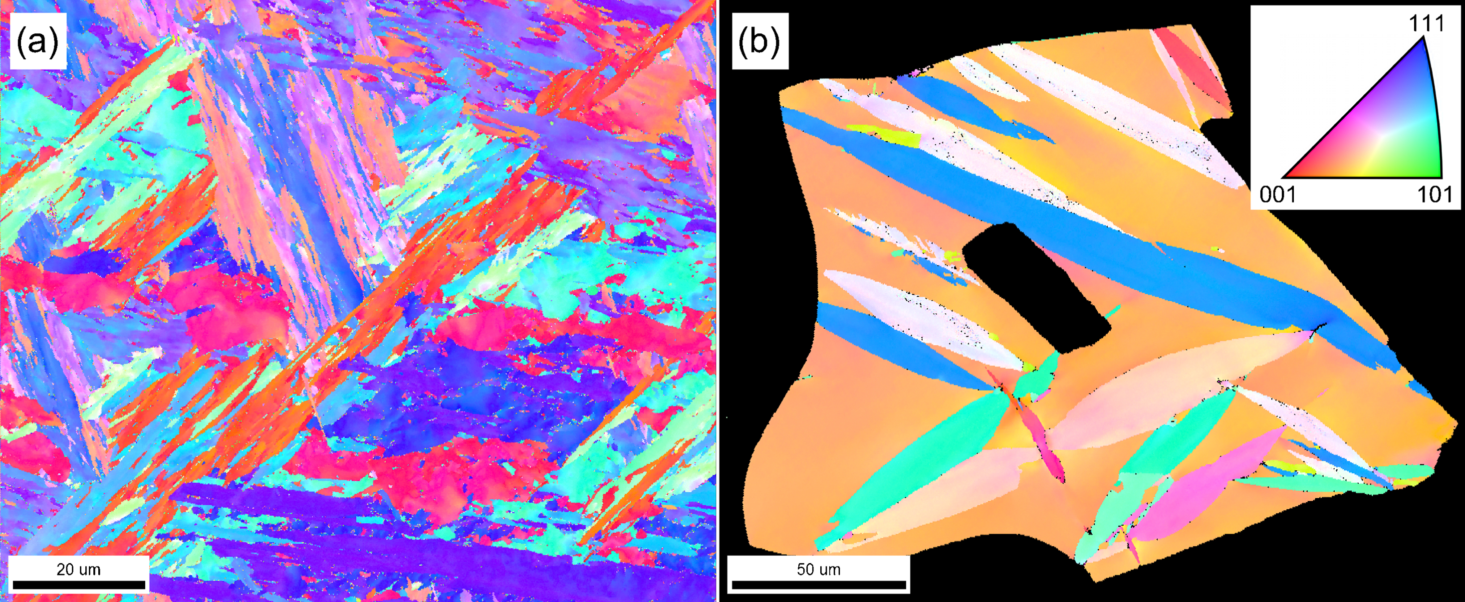
a FV535 tempered martensitic steel (99 martensite); b Fe–30 at-Ni alloy. In b, large orange area is fcc parent phase and lenticular features are martensite
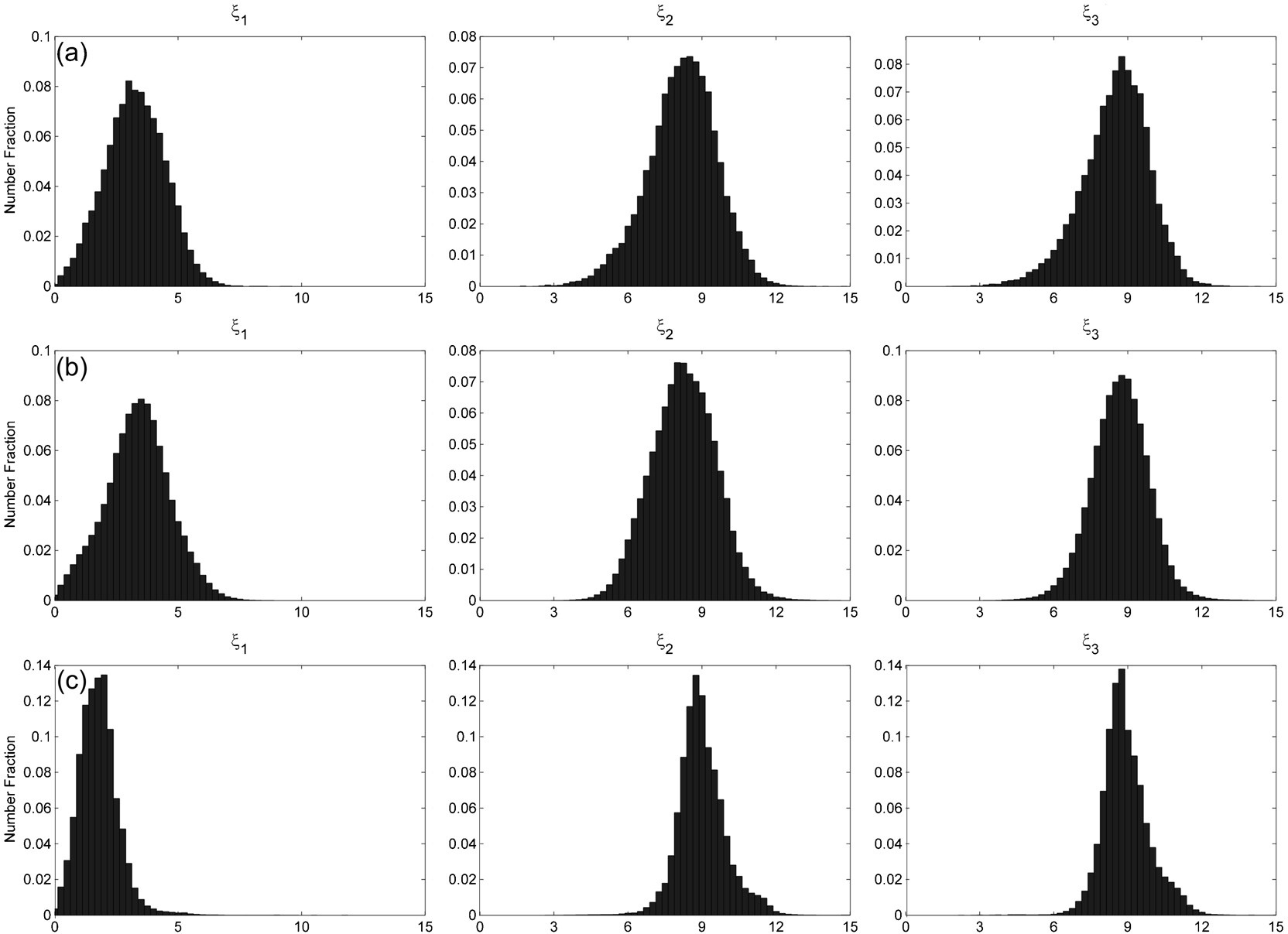
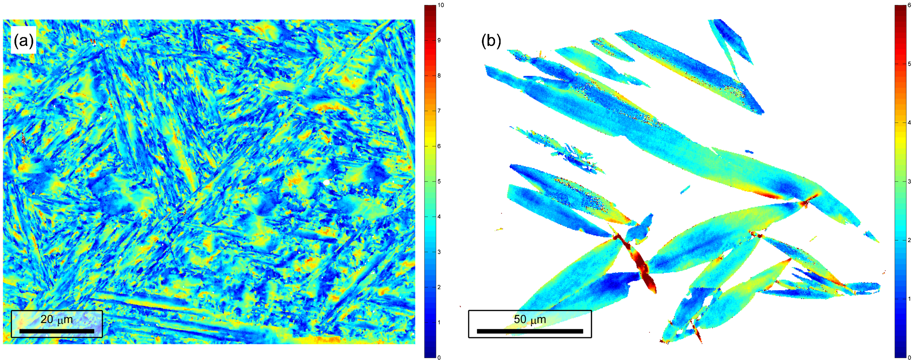
Figure 3a, b and c shows the distribution of the three angular parameters ξ1, ξ2 and ξ3 for the low-carbon steel, FV535 steel and Fe–30Ni alloy respectively. One of the most striking features of these histograms is the smoothness and near-Gaussian appearance of the distributions. The clearest difference to be observed between the three datasets is in ξ1; in the in the Fe–30Ni alloy, the peak is much closer to ξ1 = 0 than for the two steels. As can be seen from Table 1, in the NW relationship ξ1 = 0 and ξ2 = ξ3; this corresponds to the collapse of two distinct variants to a single one as observed in Fig. 1c. It should be noted, in consideration of these histograms, that for a random distribution of orientations, the distribution of misorientation angles is not in fact uniform, as is shown by the well-known work of Mackenzie and Thomson.24,25 In particular, for small misorientation angles, the frequency of occurrence of the angle increases monotonically with the angle itself. This property of the distribution must be taken into account when attempting to obtain characteristic values of the ξ1, ξ2 and ξ3 angles for a material. The simple approach used in the present work was to fit an orientation distribution function (ODF) to the set of RBRs obtained as described in the item (iv) in the section on ‘Extraction of parameters from EBSD datasets’, and to obtain the modal value of this ODF, using MTEX. 22 The modal orientation was then converted back to a rotation matrix and the arccosines of its diagonal elements taken as the characteristic values of ξ1, ξ2 and ξ3. Illustrative results obtained using a de la Vallee Poussin kernel with a half-width of 0·5° are shown in Table 2. It can be seen that the modal values are somewhat smaller than the peaks observed in Fig. 3, as would be expected if the distribution of interest is superposed on a Mackenzie-type distribution. The ξ1 values suggest that the OR in Fe–30Ni alloy is somewhat closer to NW and those in the steels a little closer to KS, but none of the sets of values in Table 2 appears to be in particularly close agreement with the values obtained from either of the two ideal OR.
Frequency distributions of angles
Values of angular parameters for three representative samples
The effects of modifying the ODF parameters, and the issue of to what extent the ξ1, ξ2 and ξ3 values obtained in this way constitute representative values for the dataset, require comprehensive investigation. A statistical treatment aimed at finding mean values directly from the misorientation angle distributions is also under development, since this may well give us more detailed information than can be obtained from fitting any type of ODF.
Spatial mapping
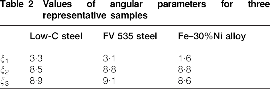
In addition to statistical treatment of aggregate data, the angular parameters can be used for mapping to investigate whether the observed variations in OR are simply random or have some correlation with position. Figure 4 is a spatial map of the values of ξ1 for the FV 535 and Fe–30 at-Ni datasets (the same as are plotted in the leftmost histograms in Fig. 3b and c. The values of this angular parameter seem to undergo spatial gradations. In Fig. 4a, contour-like gradations occur across regions that correspond to the individual martensitic variants in the substructure (which can be recognised by their different colours in Fig. 2a); typically, values of ξ1 tend to be smaller in the centre of a variant and larger towards the edges. The martensite in Fig. 4b also exhibits variations in its ξ1 value across individual plates with particularly extreme values at points where plates impinge against one another. What, if anything, these variations may have to do with the mechanism by which the martensite was formed, the dislocation density and the reorganisation processes occurring during tempering in the case of FV535, is still unclear. However, what does seem clear is that the variations observed on the pole figure are not simply random experimental scatter, since this would result in a speckled appearance rather than the observed smooth gradations.
Spatial distribution of angle ξ1 in a FV535 steel and b Fe–30 at-Ni alloy. Legend units are degrees
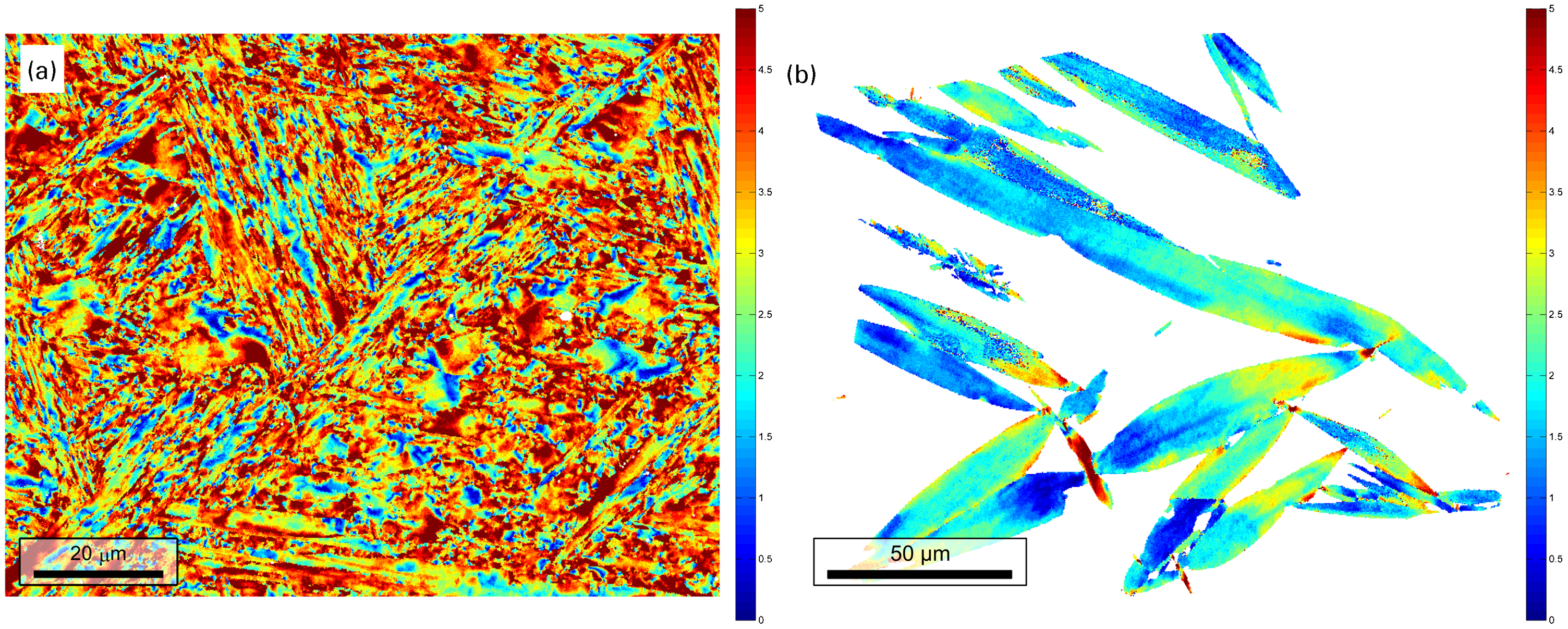
The FV 535 dataset was further processed to obtain a map showing the angular deviation from the ideal Kurdjumov–Sachs OR (Fig. 5a) and the Fe–30 at-Ni processed to show the angular deviation from the ideal Nishiyama–Wassermann OR (Fig. 5b). Smooth, spatially correlated variations are again in evidence. While there are some areas in Fig. 5a, appearing in dark blue in the image, where the OR is close to KS, the map is not composed of the discrete bright and dark areas that might be expected if a mixture of exact KS and exact NW variants were present, as had been suggested in an earlier study. 13 (A plot of the deviation of the OR from NW, not shown here, demonstrates in addition that some regions with OR far from KS are relatively close to NW, while others can be deviated by up to 5–6° from both.) Instead, it appears that at least on this length scale, a continuous range of orientation relationships exists. In a similar way, Fig. 5b demonstrates that some parts of the martensite plates have OR close to NW, but deviations from this occur in a continuous manner within plates. One possible explanation of the deviations is that the OR between the martensite and the austenite from which it forms is constant; the first martensite to nucleate forms with this OR, but the shape deformation caused by this transformation rotates the surrounding austenite, such that the next martensite to form grows from a slightly differently oriented parent. However, this explanation remains speculative until studies of the early stage of the transformation can be carried out.
Spatial distribution of angular deviation from a ideal Kurdjumov–Sachs orientation relationship for FV535 steel and b ideal Nishiyama–Wassermann orientation for Fe–30 at-Ni alloy. Legend units are degrees
Orientation relationships determined from experiment are not only of theoretical interest; they can also be applied to gain understanding of how lath martensitic microstructures, such as those in FV535 and related alloys, change during exposure to high temperatures and/or stresses. The special OR between the martensite and its parent austenite gives rise to a limited set of orientations between the different martensite variants arising from a single prior austenite parent. Based on a knowledge of lath martensite morphology and crystallography, the boundaries can be classified and the extent of coarsening in each type of substructural unit can be investigated. (For a more detailed description of this approach and some results, the reader is referred to Ref. 26.)
Conclusion
The present work discusses the use of three angular parameters, first presented by Kurdjumov and Sachs, as a way of representing orientation relationships. The main advantages of this representation are the simple separation between material-specific and symmetry-related parts of the OR, the relative ease with which OR data can be extracted even from large EBSD datasets and the way in which experimental OR can be compared with theoretical OR and spatially plotted. The variation previously observed in pole figures from ferrous martensitic materials is associated with rather smooth frequency distributions of the angular parameters and these variations do appear to be related to the martensitic morphology rather than simply being attributable to measuring errors or grain-size-related artefacts in the EBSD system. It is not yet understood how, if at all, the variations in observed OR may be related to the mechanism of martensitic transformation. Nonetheless, the OR parameters can be put into use to follow microstructural changes resulting from exposure to high temperatures and stresses.
Footnotes
Acknowledgements
E. J. Payton gratefully acknowledges support from the Adolf Martens postdoctoral fellowship program for the portion of this work which was initiated at the Bundesanstalt für Materialforschung und –prüfung, 12205 Berlin, Germany. V. A. Yardley wishes to thank the Deutsche Forschungsgemeinschaft for financial support through the grant ‘EBSD Investigations of crystallographic orientation scatter in the martensitic transformation (YA 326/2-1)’. The authors would additionally like to thank MTU Aero Engines GmbH and Professor H. K. D. H. Bhadeshia for the provision of samples and Ms S. Fahimi, Mr P. Thome and Professor T. Tsuchiyama for permitting the use of their experimental datasets in the present work.