
Abstract
In the last decade there has been a breakthrough in the construction of theories leading to models for the simulation of atomic scale processes in steel. In this paper the theory is described and developed and used to demonstrate calculations of the diffusivity and trapping of hydrogen in iron and the structures of carbon vacancy complexes in steel.
Keywords
Historical introduction
In 1947 Geoffrey Raynor wrote ‘if metallurgists of this country do not learn about the electron theories they may discover too late, that the industry in other countries has benefited from knowledge of modern theories and is developing new alloys.’ Hume-Rothery and Raynor had understood perfectly from the work of Mott and Jones before the war that to unravel the complexities of metal phase diagrams required the powerful methods of metal physics that had arisen out of the new quantum mechanics of Schrödinger and Heisenberg of the 1920's. 1 However, some 15 years later, Hume-Rothery writes ‘The work of the last ten years has emphasised the extreme difficulty of producing any really quantitative theory of the electronic structure of metals, except for those of the alkali group.’ The breakthrough came just a few years after that with the appearance of the density functional theory (DFT) of Kohn and co-workers2,3 and for which Walter Kohn shared the Nobel Prize in Chemistry (with John Pople) in 1998.
It was understood then, and is understood now, that what holds together the atoms in a metal are the valence electrons. These act as the ‘glue’ which is ultimately responsible for the properties that we exploit in metallurgy to produce alloys of prescribed hardness, ductility, fracture resistance, and so on. What Hume-Rothery meant by electronic structure is the stationary state solutions of the Schrödinger equation for the electrons in condensed matter moving in the (so called ‘external’) potential of the fixed nuclei. At issue in the 1960's was the awareness that this was fundamentally a many electron problem, requiring the knowledge of a wavefunction  which depends on the positions and spins of all the N electrons involved. On the other hand, every student learns quantum mechanics in terms of a Schrödinger equation whose solution, ψ(r,s), is the wavefunction of a single particle moving in an electrostatic potential, V(r), which at most includes the potentials of all other interacting particles in some average way. Because the electron–electron interaction is due to the long ranged Coulomb force it was thought inconceivable that a ‘one-electron’ theory would yield useful results for the electron gas in metals, and therefore it was a bold move by physicists even to attempt this approach.
Density functional theory
The principal discovery in the DFT was that the ground state energy of a many electron system is uniquely determined by the electron density alone, meaning that it is not necessary to find the complicated many electron wavefunction. 2 Moreover it was found that the many-electron Schrödinger equation could be cast exactly into one-electron form if the potential V(r) is regarded as an effective potential including a contribution called ‘exchange and correlation’ which includes all the complicated electron–electron interactions. 3 The problem is only solvable, however, if one makes an approximation to this exchange–correlation potential; this is the local density approximation (LDA) which asserts that every electron sees the potential due to other electrons as if it were living in a uniform electron gas, whose density is taken as that density which the electron momentarily encounters.
For two reasons the DFT did not make immediate impact in the world of metallurgy and solid state physics. First the LDA was received with great scepticism since it seemed to be sweeping a great deal of the essential physics under the carpet. Second the solution of the ‘self consistent problem’ requires a fast computer and complicated computer program. ** The first problems solved were to calculate the electronic structure itself, especially energy bands and Fermi surfaces; and it was not until it was possible to calculate the total energy and compare crystal structures, calculate heats of formation and elastic constants which could be compared to experiment that it was realised that the LDA was an approximation that was much better than it ought to have been. To jump some four decades ahead, it is now fully accepted that the LDA is able to predict structural properties of metals and alloys, to compute interatomic forces and to make atomistic simulations, including molecular dynamics (MD) at least for a few tens of atoms over a few picoseconds of simulation time.
Tight binding theory
The previous sentence gives the clue as to why the LDA cannot be expected to be the final word in atomistic simulations. Evidently if one wishes to make large scale MD simulations or molecular statics relaxations to study processes such as diffusion, dislocation core structures and mobilities, the current recourse is to so called classical interatomic potentials, for example the well known embedded atom method. 4 Classical potentials display a number of unrepairable difficulties. They cannot describe magnetism (essential for the study of iron and steel); they cannot account for metals with negative Cauchy pressure; and in all but a few exceptional cases they fail to reproduce properly the core structure of dislocations in α-Fe. 5
There is however a middle way, and this is the tight binding (TB) approximation. TB is a fully quantum mechanical approach to the electronic structure calculation and yields total energy and interatomic forces that can be used in MD simulations. On the other hand it is much faster computationally than the LDA because the hamiltonian is not constructed from first principles; instead a look up table of hamiltonian matrix elements is created by fitting certain fundamental parameters to experiment and to accurate density functional calculations.6,7 There is a deeper fundamental theory behind the TB approximation that goes beyond the notion of a fitted semi-empirical scheme. A number of authors have shown that the TB approximation can be derived directly from DFT using the notion of first order and second order expansions of the Hohenberg–Kohn total energy functional in the difference between some assumed input charge density and the actual self consistent density.8,9,6 TB can describe itinerant magnetism in transition metals using the self consistent Stoner-Slater theory 10 and successful models have now been constructed for α-Fe and γ-Fe, both pure, and containing interstitial impurities, hydrogen and carbon.11,12
Atomistic modelling of processes in steels
It is only in the last decade that metal physicists have come around to tackling the problem of interstitials in Fe. Only once the case of C in Fe is solved can one be said to be able to model processes in steel. There are a few classical potentials, to describe both H and C in α-Fe,13–15 but these are prone to the same difficulties as those outlined above for pure iron, in addition to which the number of fitted parameters rises dramatically so that for example the H–Fe interations require more than 40 parameters with which to be described. 13 Therefore it is very instructive to determine what can be done using the ‘middle way’ tight binding approximation. This is followed through in the examples in the next sections.
Hydrogen in α-Fe
In some sense H is the most interesting of the intersitial impurities because of its small atomic mass. This fact coupled with the geometry of the bcc lattice leading to a rather small activation energy for diffusion between tetrahedral interstices means that the hydrogen atom, or proton, cannot in general be treated as a classical particle. A hydrogen molecule is characterised by a rather strong covalent bond arising from the splitting of the atomic H-1s level into bonding and antibonding molecular orbitals; only the bonding levels are occupied (by two electrons) and antibonding orbitals are unoccupied. 16 This situation changes when the H2 molecule finds itself at the surface or within a transition metal. In that case the H-1s levels are lower in energy than the bottom of the transition metal d-bands and so both the bonding and antibonding levels become occupied: the covalent bond breaks apart and the H atom is free to move about the crystal lattice. It makes sense to think of the H-atom as a freely moving proton that has given up its electron to the energy bands of the solid. Since the H-1s orbitals are fully occupied it is tempting to think of the H-atom as negatively charged, that is H−, but this is not really helpful as any charge in a metal is very efficiently screened by the conduction electrons. The proton in solution in α-Fe occupies the tetrahedral interstices. The quantum nature of the proton is illustrated in Fig. 1. Here the TB method 11 has been used to map out the so called minimum energy path 17 for the proton to move from its tetrahedral site to a neighbouring site. In the process the proton passes through a maximum in the energy along that path; in fact this is a saddle point in the total energy landscape as understood from classical theory of diffusion. 18

Minimum energy path for proton migration in α-Fe: open circles show energy as function of proton position in Å as it moves in potential well around tetrahedral interstice; dotted line is parabola fitted to points; curve labelled
is graph of gaussian wavefuncion of proton moving the harmonic oscillator potential;
19
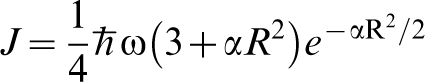
horizontal line marks zero point energy relative to bottom of well; this is energy of ground state of proton, which in periodic potential of lattice of tetrahedral sites forms band of states of width on order of hopping integral J (equation (1)) as indicated by horizontal dotted lines
The dotted line in Fig. 1 is a parabola fitted to the calculated energy showing that to a good approximation the proton is moving in a quadratic potential. This means that it possesses the wavefunction of a harmonic oscillator, namely the normalised gaussian
19
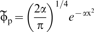
In Fig. 1 is shown the proton wavefunction  , the zero point energy
  , and the magnitude of the hopping integral J. Several points are notable. The zero point energy is large on the scale of the energy barrier so that the proton does not occupy the energy at the bottom of the potential well as would a classical particle, instead even in the ground state the proton possesses an energy nearly half way up to the saddle point. If we think of the energy curve as a portion of a periodic potential, then it is clear that at zero temperature, the proton occupies a Bloch state or energy band whose width is on the order of J. Both these facts lead to the conclusion that a classical approach to the diffusivity of H in α-Fe is likely to lead one into error.
Hydrogen diffusion in α-Fe
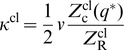
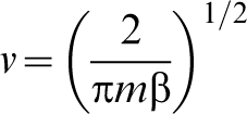
In the classical approach to diffusion, the so called transition state theory, one is interested in the classical rate constant κcl, which can be expressed in terms of a ratio of partition functions.18,22 We are interested in the ‘reactant state’ in which the diffusing atom occupies a lattice, or interstitial, site and its partition function is denoted  . The second partition function of interest concerns the particle at the saddle point. Following Vineyard
18
we construct a constrained partition function
. The second partition function of interest concerns the particle at the saddle point. Following Vineyard
18
we construct a constrained partition function  , in which the asterisk on the reaction coordinate q, conveys the fact that it is confined to the dividing surface in configuration space: this is the surface perpendicular to the minimum energy path. This reduces the dimensions of the configuration space available to the particle by one. We then have18,23
Exactly the same formula applies in the quantum transition state theory if one simply replaces the classical partition functions with their quantum mechanical counterparts.
23
The way to calculate quantum mechanical partition functions is to use Feynman's path integral formalism.
30
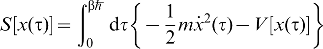
A very readable account can be found in Ref. 31. Feynman shows that the partition function at temperature T of a single particle moving in a potential V(x), in one dimension for simplicity, is
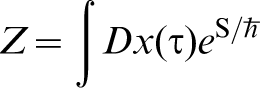
 .
30
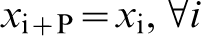
In general a path is such that the particle starts out at position x1, say, at τ = 0, that is, having infinite temperature, and travels to position x2 at the temperature T at which we require the partition function. However for the purpose of calculating Z the only paths included in the integral are those for which the position of the particle is the same at τ = 0 and
.
30
In general a path is such that the particle starts out at position x1, say, at τ = 0, that is, having infinite temperature, and travels to position x2 at the temperature T at which we require the partition function. However for the purpose of calculating Z the only paths included in the integral are those for which the position of the particle is the same at τ = 0 and  so that these are closed paths in that sense. Therefore, equation (3) is the integral of
  taken over all positions x and all paths for which the particle travels from x and back again in an ‘imaginary’ time
  which is determined by the temperature of interest. In equation (3)
 .
32
.
32
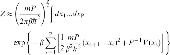
If one discretises the closed paths into P segments, then the partition function can be approximated to
31
 .
32
What is astonishing about this formula is that the partition function of a quantum mechanical particle is equivalent to the classical partition function belonging to a necklace of P beads connected by harmonic springs of stiffness
.
32
What is astonishing about this formula is that the partition function of a quantum mechanical particle is equivalent to the classical partition function belonging to a necklace of P beads connected by harmonic springs of stiffness 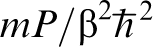 . Each bead feels a potential energy V(r)/P. The numerical estimate converges to equation (3) when the discretisation parameter P is chosen to be large enough.
Armed with the approximate partition function, these can be substituted for the classical functions in equation (2) to obtain the rate constant  in the quantum transition state theory.
23
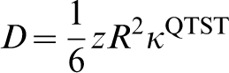
Finally the diffusivity can be obtained from the Einstein formula, assuming an uncorrelated random walk among the tetrahedral sites of the bcc lattice
22
in the quantum transition state theory.
23
Finally the diffusivity can be obtained from the Einstein formula, assuming an uncorrelated random walk among the tetrahedral sites of the bcc lattice
22
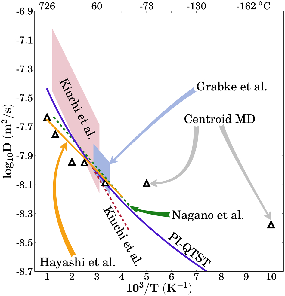
Diffusion coefficients of H in α-Fe calculated by path integral quantum transition state theory (PI QTST): 24 bands of data represent assessment by Kiuchi and McLellan 25 of hydrogen gas equilibration experiments and measurements by Grabke and Rieke, 26 vertical width of band reflecting reported error bars; remaining lines are data from electrochemical permeation experiments, assessed by Kiuchi and McLellan 25 and measured by Nagano et al.; 27 and measurements using gas and electrochemical permeation by Hayashi et al., 28 extent of each data set represents temperature range over which assessment or measurements are reported; triangles show theoretical results from centroid molecular dynamics calculations using classical interatomic potential and are taken from Ref. 29
Even though it is necessary to treat the motion of the protons in steel quantum mechanically this does not mean that the classical minimum energy path is unimportant. On the contrary, as has been indicated above, the quantum mechanical approach to tunnelling requires knowledge of the classical activation energy. Moreover it must be understood that the computation of the classical minimum energy path (that is, treating the nuclei as classical) is still a quantum mechanical calculation if tight binding or density functional theory is used to calculate the interatomic forces.
Hydrogen trapping at vacancies
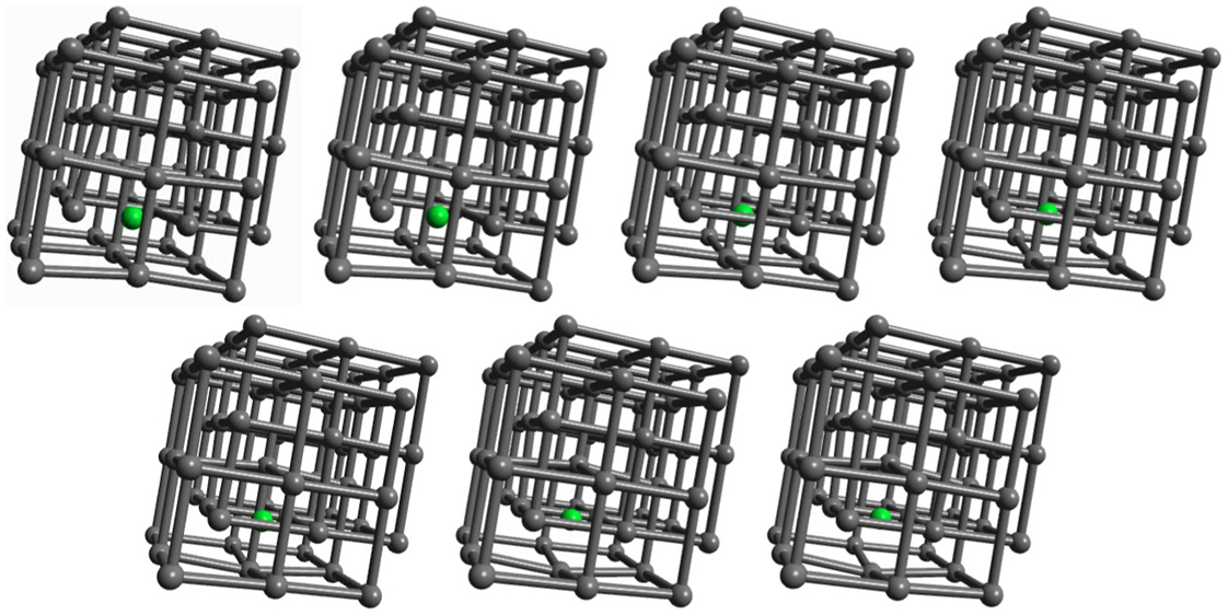
We can extend the study of hydrogen in the perfect bcc lattice to consider its interaction with vacancies. This is of great technological importance as hydrogen induced superabundance of vacancies is thought to be a mechanism of hydrogen embrittlement.33,34 Figure 3 shows minimum energy paths for H atoms migrating from a neighbouring unit cell into a unit cell containing an iron vacancy in α-Fe. We show successive paths as first one, then two, then three, up to the case where five H atoms have been absorbed by the vacancy. For illustration, the atomic structures of the initial and final state are shown for the case ‘5H’ in Fig. 4.
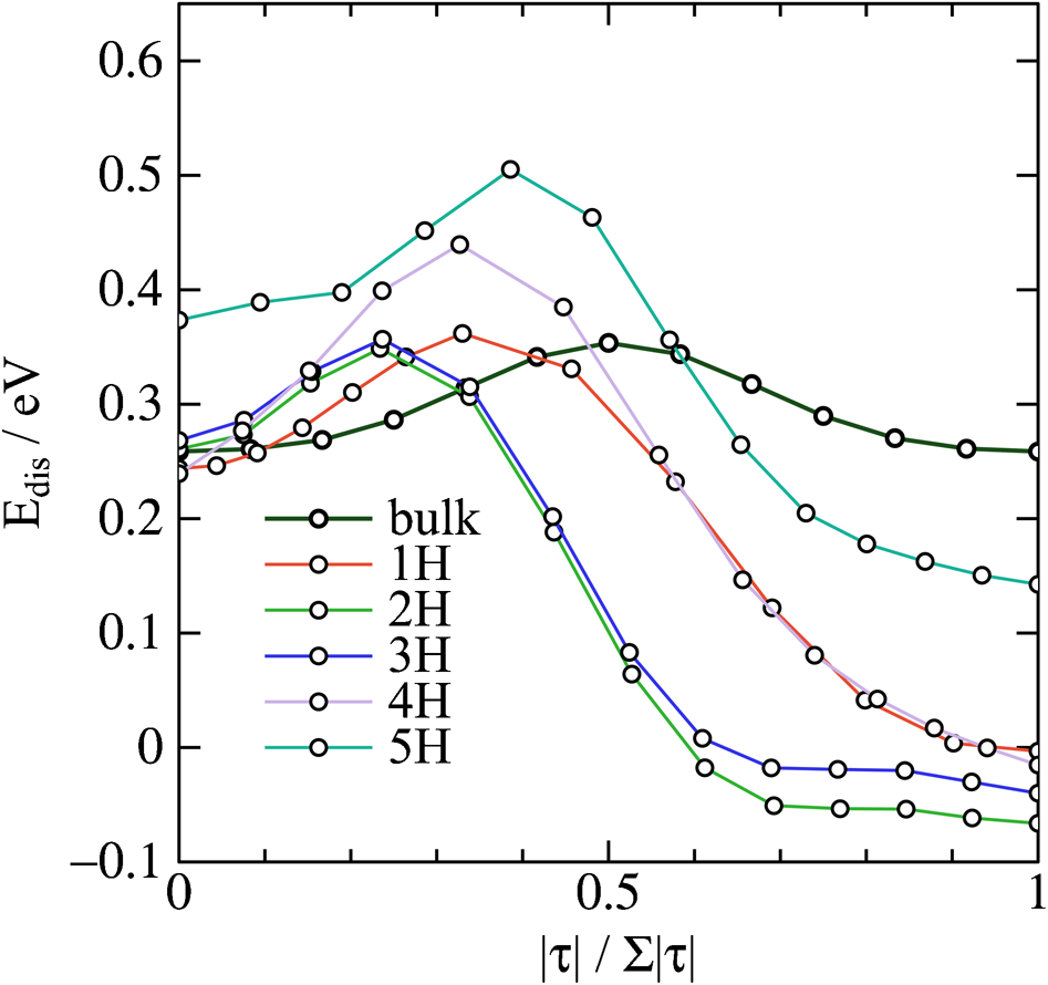
Calculated minimum energy paths for hydrogen migration to vacancy in α-Fe: each curve, labelled nH corresponds to case where already n−1 H atoms have been absorbed at vacancy; curve labelled ‘bulk’ is same minimum energy path as shown in Fig. 1; ‘reaction coordinate’ along abscissa shows fractional length of total path, or length in configuration space of ‘nudged elastic band’, 17 which is different for each case; for example two end points (zero and one on abscissa) illustrated in terms of their atomic structure for case of five H atoms are drawn in Fig. 4
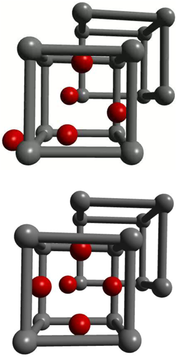
Atomic structures of two end points of minimum energy path labelled ‘5H’ in Fig. 3; at start of path, there are four H atoms already trapped by vacancy occupying near-tetrahedral sites at faces of cube, and there is one proton in near-bulk tetrahedral site in unit cell to left; at end of path (lower figure) that proton has migrated into fifth near-tetrahedral site at vacancy that has now trapped five protons
The energy plotted in the ordinate of Fig. 3 is the ‘dissolution energy’, namely the total energy of the α-Fe crystal containing hydrogen compared to an equivalent perfect crystal and the same amount of hydrogen in the H2 gaseous state.13,11 In the case of hydrogen migration in perfect bulk α-Fe, labelled ‘bulk’ in Fig. 3, this is always positive, reflecting the fact that hydrogen is very insoluble in α-Fe. Figure 3 shows that hydrogen atoms can lower their potential energy by becoming absorbed at a vacancy and in the case where two or three H atoms are trapped the dissolution energy is negative. This observation is extremely significant in supporting the notion that vacancies act as traps for H atoms. Hydrogen traps deeper than about 0·5 eV are often said to be irreversible, that is one would not expect any significant thermal desorption at temperatures up to 300°C. 35 Under this classification we see that the vacancy in ferrite acts as a reversible trap for hydrogen. Figure 3 also shows that up to five H atoms can be transferred exothermically from bulk tetrahedral sites to a single vacancy. This result is consistent with experiment 36 and with DFT calculations. 37 On the other hand a quantitative comparison is less convincing. Myers et al. 38 have assigned trap depths of 0·43 and 0·63 eV to respectively 3–6 and 1–2 deuterium atoms trapped at a vacancy in α-Fe. In that case the trend is the same as in the theory, but the magnitudes are at odds with it. In particular, we find in Fig. 3 that the trap depth is about the same, 0·25–0·3 eV, for all cases up to four H atoms. The so called superabundance of vacancies 36 is an example of what has been called the ‘defactant’ effect by Kirchheim. 39 This is in analogy with the usage surfactant to describe a chemical which acts to lower the free energy of a surface; here the hydrogen species acts to lower the free energy of formation of the vacancy defect by becoming trapped within it.
Carbon in α-Fe
One might well ask whether there is a defactant effect at work due to interactions between carbon atoms and vacancies in steels and whether this has implications for heat treatment and microstructures in martensite and bainite. As yet this question is unresolved, 40 although there have been some very interesting DFT calculations by Först et al. 41 which can answer this question. These authors showed that a number of defect complexes exist in steels comprising carbon interstitials and vacancies. According to their calculations, the two predominant point defects at 160°C, apart from alloying impurities, are the carbon interstitial in octahedral sites and a vacancy having two carbon atoms bound to it. This rather startling result plainly has huge implications for the understanding of both carbon and self diffusivity in α-Fe.
Recently a tight binding model for carbon in magnetic α-Fe has been demonstrated and this can be used to good effect to reproduce this result and to give an interpretation. 12
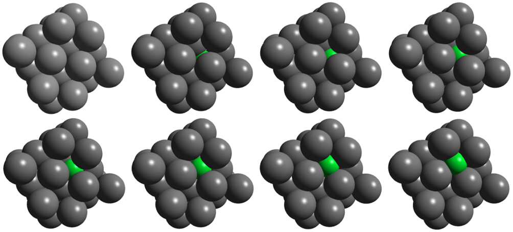
Some calculated data relevant to carbon in steel are shown in Table 1 in which tight binding results are compared to DFT and to experiment. The TB model employs the Slater–Stoner theory of collinear itinerant magnetism 10 and so non collinear effects are not captured; this may lead to small errors in the treatment of γ-Fe. 46 The experimental vacancy formation and migration energies are, surprisingly, still very controversial; here we follow the discussion by Seeger and quote his results. 45 The TB migration energies for C in ferrite and austenite are in quite good agreement with DFT results. C migration in α-Fe is illustrated in Fig. 5. This shows rather clearly the local tetragonal strain intoduced into the lattice by the C interstitial. This can be modelled as a double Boussinesq force without couples 47 and gives rise to an elastic dipole which can interact with a second rank tensor, stress field, in close analogy with a electric dipole which responds to a vector, electric field. 48 Figure 5 shows rather clearly how the elastic dipole reorients through 90° after each hop. In austentite the carbon atom has a choice of migrating between octahedral sites via an intermediate tetrahedral site or it may take the direct route by forcing its way through the centre of the nearest neighbour Fe–Fe bond. As the energies in Table 1 show the carbon, rather surprisingly, chooses the second option; the minimum energy path is illustrated in Fig. 6.
Atomic structure snapshots of calculated minimum energy path for carbon diffusion in perfect α-Fe: it can be seen that in first image elastic dipole points roughly left to right as crystal is locally tetragonally distorted by carbon atom occupying irregular octahedron of perfect bcc lattice; as point defect moves dipole rotates into up and down direction in the figure; that is, dipole originally along x-axis rotates 90° into z-axis; elastic interaction between point defects will be such as to cause these to align in analogy with alignment of spins in ferromagnetic material,49,48 it is this effect that leads to tetragonality of martensite and bainite50,51
Atomic structure snapshots of calculated minimum energy path for carbon diffusion in γ-Fe; surprisingly C atom does not take intermediate hop via neighbouring tetrahedral site for which activation energy is 2·1 eV (Table 1); instead it forces its way through nearest neighbour Fe–Fe bond at so called high energy ‘d’-saddle point 12 for which energy barrier is very much smaller: 0·63 eV
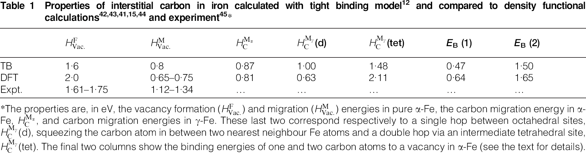


*The properties are, in eV, the vacancy formation ( ) and migration (
 ) energies in pure α-Fe, the carbon migration energy in α-Fe,
  , and carbon migration energies in γ-Fe. These last two correspond respectively to a single hop between octahedral sites,
  (d), squeezing the carbon atom in between two nearest neighbour Fe atoms and a double hop via an intermediate tetrahedral site,
  (tet). The final two columns show the binding energies of one and two carbon atoms to a vacancy in α-Fe (see the text for details).
Finally, we can turn to the question of the binding of carbon interstitials to a vacancy in α-Fe. The data in the last two columns of Table 1 show a quantity EB defined by Becquart et al. 14 This is the total energy of a defect complex compared to the energy of the constituent point defects when widely separated. Therefore, for example, EB(2) is the energy of an isolated vacancy and two carbon interstitals minus the energy of two carbon atoms bound to a vacancy. A positive value means that the complex is more stable, in this case by 1·65 eV, than its separated components. In other words the crystal gains 1·65 eV (159 kJ mol−1) when two carbon atoms become bound to a bare vacancy. We have seen in the case of hydrogen that first, the H atom does not occupy the actual vacant site that entails a large energy penalty. 37 Instead the H atoms occupy near-tetrahedral sites in the cube faces surrounding the vacancy. Second, we have seen that a vacancy in α-Fe will absorb up to five H atoms out of solution exothermically; moreover the configuration with two or three trapped H atoms actually has a negative heat of solution with respect to hydrogen gas. Carbon also does not occupy the actual vacant site, substitutional phases of carbon in Fe have very large, positive heats of formation. 12 Instead carbon atoms could occupy up to the six octahedral positions at the centres of the faces of the cube surrounding the vacant site. 41 Of the six possible Fe-vacancy–C-interstitial complexes, the cases of two and three carbon atoms have the greatest binding energy 41 as indicated in Table 2, hence the prediction that the vacancy plus two carbon atoms is the next most predominiant defect after the isolated carbon interstitital in Fe–C alloys. 41
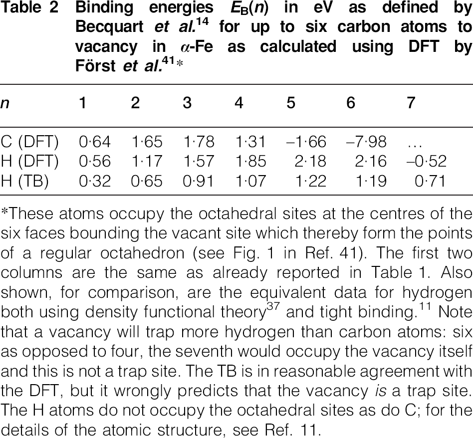
*These atoms occupy the octahedral sites at the centres of the six faces bounding the vacant site which thereby form the points of a regular octahedron (see Fig. 1 in Ref. 41). The first two columns are the same as already reported in Table 1. Also shown, for comparison, are the equivalent data for hydrogen both using density functional theory 37 and tight binding. 11 Note that a vacancy will trap more hydrogen than carbon atoms: six as opposed to four, the seventh would occupy the vacancy itself and this is not a trap site. The TB is in reasonable agreement with the DFT, but it wrongly predicts that the vacancy is a trap site. The H atoms do not occupy the octahedral sites as do C; for the details of the atomic structure, see Ref. 11.
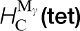
The reason for the large stability of the vacancy plus two carbon atoms can be seen in Fig. 7 which shows four possible configurations of the two carbon atoms bound to the vacancy that have been proposed.52,41 The structure labelled (a) is perhaps the most obvious, but in fact it has the highest potential energy. What is predicted to happen is the that the carbon atoms approach each other to form a covalent bond, whose bond length is 1·43 Å which is the same as the bond distance in diamond. The structure is therefore that of a C2 dimer bound to the vacancy. The structures labelled (b)–(d) in Fig. 7 correspond to possible orientations of the dimer and in fact, as predicted both in DFT and in tight binding it is the structure labelled (d) that has the lowest potential energy. 12 The reason for this can be seen in Fig. 7. In this orientation each carbon atoms makes four bonds, one to the other carbon atom to form the dimer and three further bonds of equal length, 3·65 Å, to neighbouring Fe atoms. In this way the carbon atom satisfies its requirement of four fold coordination. This is an example in which a quantum mechanical theory is expected to be essential if the phenomenon is to be correctly described, because the bonding is achieved by the well known sp-hybridisation of the carbon atomic orbitals. 16
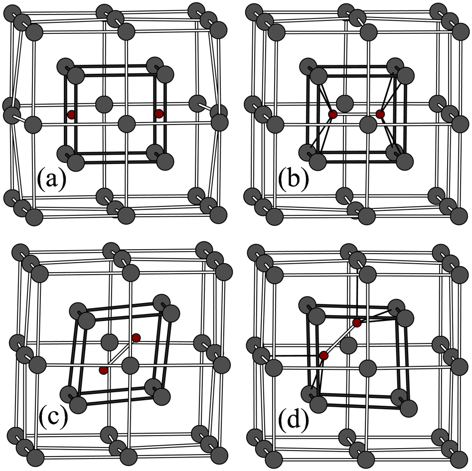
Four possible atomic structures52,41 of carbon dimer bound to vacancy in α-Fe calculated by static relaxation using tight binding interatomic forces: 12 all four are local minima in potential energy; note that in all but case a two C atoms have joined together to form C2 ‘dimer molecule’ inside vacancy; global minimum is predicted to be structure labelled d because that offers preferred four-fold coordination of carbon atom, exactly as it experiences in ethane molecule, although here of course bonds are to Fe, not H atoms; see text for discussion
Conclusions
The aim of this paper has been to show how electronic structure calculations can be made that have direct relevance to physical metallurgy. The state of the art is the density functional theory, but it has been demonstrated that an abstraction into a tight binding model can be both reliable and predictive. This means that in the future it will not always be necessary to rely on the somewhat uncontrollable approximations attendant upon simulations using classical potentials. In particular it is now possible to make atomistic models of total energy and interatomic force in magnetic iron and steel. In the present case this has been applied to the calculations of atomic and electronic structures of hydrogen and carbon interstitials in iron. This has resulted in new insights into the nature of vacancies as traps for hydrogen and carbon and it is expected that this will have future impact in the understanding of hydrogen embrittlement and processes in the heat treatment of steel, leading ultimately to the design of new materials.
Footnotes
Acknowledgements
**
In casting the many-electron problem into one-electron form it happens that the effective potential comes to depend on the electron density which is the square of the one-electron wave function. In that way the potential that enters the Schrödinger equation depends on its solution. This means that one needs to seek a self-consistent solution to the problem that can only be done with a computer.