Sage Journals: Discover world-class research

Abstract

Conventional open pit mine design methods ignore geological uncertainty in terms of metal content and material types which can impact the quantities processed in multiple process mining operations. A stochastic framework permits the use of geological simulations to quantify geological uncertainty; however, existing models have either not been extended to pushback design for mines with multiple elements, multiple materials and multiple destinations, or are limited in their ability to incorporate joint local uncertainty represented through sets of geological simulations. This work aims to integrate grade and material uncertainty in pushback design for open pit mines. Two formulations are proposed to modify existing pushback designs to reduce risk in terms of the amounts of material going to each destination, while maintaining similar pushback sizes when compared to the original design. The proposed formulations are applied at BHP Billiton's Escondida Norte mine, Chile, and show a 35–61% reduction in variability in terms of quantities of material sent to the various processes.

Keywords

Open pit mine design Simulated annealing Geological uncertainty Phase design Multiple processes Multiple materials

Introduction

The objective of pushback (or cutback or phase) design is to provide a long term guide for the sequence of extraction of material from an open pit mine over time such that the net present value (NPV) of the mine production schedule is maximised (Hustrulid and Kuchta, 2006; Dagdelen, 2007). Conventional mine design and production scheduling (Lerchs and Grossmann, 1965; Picard, 1976; Whittle, 1988; Tachefine and Soumis, 1997; Hochbaum and Chen, 2000) is a stepwise procedure that only considers a single input model consisting of the expected metal content for a block of material. In the case of complex deposits, the input models may consist of various material types, which define the set processing destinations that the rock can be sent to, along with zones that require different slope angles to ensure wall stability.

As the complexity of the deposit increases in terms of number of elements (metals, deleterious elements), materials and candidate destinations, the conventional framework for mine design fails in the sense that it only sees an expected value for each element and material type and does not consider the interactions of the uncertainties between the grades and material types and the compounded effect that it may have on the various processing paths and the final economic value of the mine design. The assumption of constant inputs for each block in the orebody model may therefore result in an unrealistic mine design in terms of practicality and ability to meet annual production targets (Dimitrakopoulos et al., 2002). Frameworks for optimisation under geological and economic uncertainty (referred herein as stochastic optimisation methods) have been developed over the past decade to address many of the shortcomings that are inherent in conventional optimisation methods.

Albor and Dimitrakopoulos (2010) integrate pushback design into the stochastic optimisation framework by considering the influence of the number of pushbacks and pushback sizes has on the risk profiles for production schedules. The authors propose grouping a series of nested pits into a specified number of pushbacks by evaluating the combinations in terms of approximated discounted economic value. The authors generate life-of-mine (LOM) production schedules for a mine design based on a varying number of pushbacks using a SIP formulation (Dimitrakopoulos and Ramazan, 2008; Ramazan and Dimitrakopoulos, 2007, 2012), and document the effects that the stepwise procedure has on the risk profiles of the production schedule. Selecting the best pushback design requires comparing the schedules for the different designs in terms of value, maximum deviations and stripping ratios over the life of the mine. By choosing an optimal pushback design, the authors are able to increase the net present value of the production schedule for a sample copper deposit by ∼30% over conventional methods; this increase is directly related to the pushback design that enables better risk management and extending the ultimate pit limits. While adding substantial value to the mine design, this framework for pushback design under uncertainty is computationally intensive, given that a SIP needs to be solved for each pushback design. The methodology is also limited by the fact that uncertainty is not directly incorporated in the pushback design but rather incorporated in the LOM production scheduling process.

Meagher et al. (2010) extend the parametric maximum flow/minimum cut approach (Picard, 1976; Hochbaum and Chen, 2000) to account for multiple orebody representations and multiple metal price simulations. The push relabel algorithm generates a minimum cut that minimises the sum of the ore left outside of the pit plus the waste mined inside. To account for multiple geological simulations, the authors introduce infinite capacity bi-directional arcs between the blocks in each of the simulations to guarantee that if a block is extracted in one simulation, it must be extracted in all simulations. By incorporating multiple simulations and applying a parameterisation, the algorithm is able to see blocks that not only have high value, but also blocks that have a high probability of being ore.

Asad and Dimitrakopoulos (2012) extend the parametric maximum flow algorithm for pushback design under uncertainty and attempt to control the relative differences in sizes between pushbacks. The authors use the subgradient method to accommodate knapsack constraints for ore quantities in the pushback (Tachefine and Soumis, 1997) and simultaneously minimise the differences in sizes between pushbacks. The authors apply the method on a copper deposit and compare the same method when solved without attempting to control the gap between pushbacks; when the gap control is used, the algorithm generates pushbacks that are much more practical (i.e. relatively equally sized pushbacks) than when the gap control is not used.

While the results thus far from the minimum cut/maximum flow framework are promising, the method is limited by its inability to simultaneously accommodate joint local uncertainty for both grades and material types that is available through the geological simulations; in the network flow framework, for any given block in a geological model, all simulations that have a positive economic value are grouped together, and all simulations with a negative economic value are grouped together, disregarding the local combinations of positive and negative blocks that any given geological simulation contains.

One alternative to using the network flow methods for pushback design is to use metaheuristics, which do not guarantee a truly optimal solution, however, can be used to find a high quality solution in a reasonable amount of time. One successful application of metaheuristics in mining is the use of the simulated annealing algorithm (Kirkpatrick et al., 1983; Geman and Geman, 1984) for LOM production scheduling under uncertainty (Godoy, 2003). Godoy proposes using an initial production schedule design and iteratively shifting blocks between production periods, with the ultimate goal of minimising deviations from ore and waste production targets. While the concept of an ore or waste production target is not directly transferable from production scheduling to pushback design (given that pushbacks can be defined over a longer and variable timescale), the methodology with simulated annealing used is general and suitable for many types of mining problems. For designing pushbacks in particular, the underlying formulation for minimising deviations and optimisation methodology using simulated annealing is directly transferrable and easily generalised for multiple processes, where the target for each destination (waste or processors) can be described by the average over all simulations.

This paper contributes a generalised stochastic pushback design algorithm that modifies an initial design to minimise the variability of the material that is sent to each destination over the geological simulations using the simulated annealing algorithm. This method is capable of optimising real world deposits, while simultaneously considering multiple (jointly simulated) elements (Boucher and Dimitrakopoulos, 2009; Rondon, 2012), simulated material types (Strebelle, 2002) that define multiple processing destinations and multiple zones with variable slope angles. The goal of the algorithm is to modify an existing pushback design to better account for the joint local uncertainty in metal grades and material types simultaneously, while remaining similar to the original design in terms of pushback tonnages and the tonnages sent to the various destinations, which indirectly leads to a reduced level of risk in the economic value of the design. The method is readily and easily incorporated into any conventional or stochastic optimisation framework, such as those previously mentioned. In the following sections, two formulations for modifying existing pushbacks that incorporate joint local grade and material type uncertainty are described, along with the implementation using the simulated annealing algorithm. The methods are then applied in a case study for BHP Billiton's Escondida Norte mine, Chile. Finally, conclusions and recommendations for future work are discussed.

Modifying pushback designs to manage geological uncertainty

The contribution of this work is a computationally efficient and general method for modifying an existing pushback design to accommodate joint local uncertainty in terms of grade and material types simultaneously for complex mineral deposits and mining chains, where the material type defines the set of destinations that the block can be sent. Two formulations are proposed to achieve this, and both are similar in nature to the formulations used for mine production scheduling using the simulated annealing algorithm (Godoy, 2003; Leite and Dimitrakopoulos, 2007; Albor and Dimitrakopoulos, 2009). Unlike the methods used for LOM production scheduling, which have specified production targets for mining equipment and destinations, pushback design is much more general and does not necessarily have consistent or constant targets for each phase. For this reason, an initial pushback design is required to specify initial targets for each phase, which can be in the form of a conventional pushback design, pit shells generated by a parametric algorithm or a randomly generated design with specified pushback size targets. The ultimate result after applying the proposed methodology is a mine design that mimics the same average tonnages in each pushback for each destination as the starting design (hence total size of pushback) and simultaneously minimises the variability of the tonnages sent to the various destinations over the set of geological simulations. Given that the variability in tonnages is strongly linked to the variability in the economic value of the material within the pushbacks, the proposed algorithm also indirectly reduces risk associated with the economic value of the design. A third formulation is proposed (see Appendix) and enables the algorithm to dynamically change the target tonnages for each destination and pushback, hence total pushback design, however, is omitted from the following discussions and is a subject of future research. The proposed methods can be easily integrated into existing frameworks for mine design and production scheduling (deterministic or stochastic), and does not drastically change the original design in terms of tonnages sent to the various destinations.

Formulations for modifying starting design

Formulation (1)

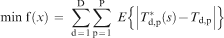
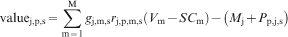
The first formulation aims to minimise the average absolute deviation (difference) from a target tonnage over all geological simulations (Strebelle, 2002; Boucher and Dimitrakopoulos, 2009), where the target for each process or destination and pushback is defined as the average tonnage over the available simulations and the starting pushback design. This formulation is similar to the objective function proposed by Godoy (2003) for production scheduling, where Godoy's ore and waste production targets are replaced by the average tonnages for each destination from the starting pushback design. The formulation for the objective function is as follows (1) where represents the indices for the destinations or processes that mined material can be sent to; represents the indices for the pushbacks; represents the indices for the input orebody simulations; represents the quantity of material (i.e. tonnes) sent to process d in pushback p in scenario s for the current (modified) pushback design; T_d,p represents the average quantity (tonnage) of material sent to process d in pushback p over all geological simulations for the initial pushback design, i.e. 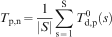and remains static throughout the optimisation process; 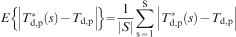represents the expected value of the deviations from the targets over all geological simulations.

Formulation (2)

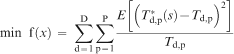
One of the potential issues that may arise with using formulation (1) is that it only evaluates changes based on a linear change in tonnage's absolute deviation. If there is a drastic difference in target quantities between the destinations, the optimiser may reduce the variability of material sent to one pushback but drastically increase the variability of material sent to another process because it is smaller in size; this is directly related to the well known volume variance subject that is studied in geostatistics (Journel and Huijbregts, 1978). Another proposed formulation is to evaluate the square deviations from the targets and standardise them by their target size. This helps to avoid the issues with large discrepancies in quantities of materials sent to the processes, and provides a better measure of the variability of material going to each process. The formulation of the objective function is as follows, and uses the same variable nomenclature as formulation (1) (2)

Implementation using simulated annealing

Given that the proposed objective functions are mathematically non-linear, metaheuristics are well suited for performing the optimisation; rather than having to define an extremely large number of precedence constraints for each block in the model that is required for traditional optimisation models, metaheuristics are able to simplify the formulation by implicitly obeying slopes and various other constraints when performing modifications to the pushback design, thus slope constraints are always respected at every iteration of the algorithm. The proposed algorithms use the simulated annealing framework to perform the optimisation based on the proposed objective functions (Kirkpatrick et al., 1983; Geman and Geman, 1984; Godoy, 2003).

Simulated annealing algorithm

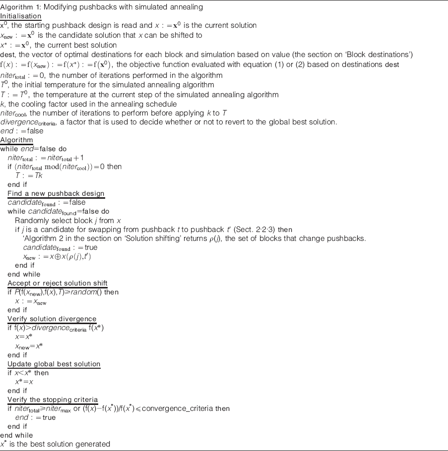
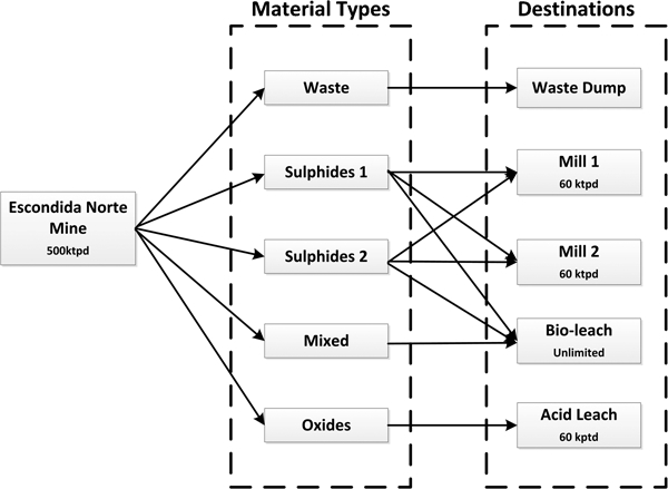
Algorithm 1 outlines the algorithm for pushback design with simulated annealing. The underlying principle of simulated annealing is to start with an initial solution, and gradually make perturbations, or shifts in the solution vector, where the probability of accepting suboptimal shifts (in terms of the variability of the design) decreases as the algorithm proceeds. Initially, the algorithm may accept suboptimal solution shifts in order to attain a better solution in a future iteration (referred to as solution space exploration). The starting pushback design is represented as an N-dimensional vector x⁰ where each component of the vector x⁰, , represents the pushback t that block j is initially assigned to. The optimal destination for each block j in each simulation is calculated by undiscounted cash value, and stored in a vector 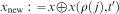dest (see the section on ‘Block destinations’). The algorithm commences with a high annealing temperature T and is gradually reduced using a cooling factor k where k<1. This temperature reduction is performed every niter_cool iterations. At each iteration of the simulated annealing algorithm, a block j is randomly selected to be shifted from pushback t to t′ (see the section on ‘Solution shifting’ for details). The updated solution vector is represented by , where x⊕x(ρ(j),t′) is the original solution with the modifications required to shift the set of blocks ρ(j) to pushback t′. 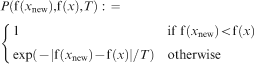The annealing algorithm then randomly accepts or rejects the shift in solution based on a probability distribution P(f(x_new),f(x),T)<rand () (3) where f(x_new) is the value of the objective function (equations (1) or (2)) for the candidate (shifted) pushback design, f(x) is the value of the objective function for the pushback design from the previous solution, and is a uniform random number. As the annealing temperature T decreases, the probability of accepting a suboptimal shift in solution, in terms of the objective function value, decreases. If the shift is accepted, the current solution x_new overwrites the previous solution x. If the current pushback design has the best objective function value discovered up to that point in the algorithm, x_new overwrites the global best solution x*. Similarly, if the optimiser is exploring a solution that is too far away from the global best solution by a factor of divergence_criteria>1, the global best solution x*, replaces the current and previous solutions x_new and x respectively.

Algorithm 1: Modifying pushbacks with simulated annealing

Initialisation

x⁰, the starting pushback design is read and is the current solution

is the candidate solution that x can be shifted to

, the current best solution

dest, the vector of optimal destinations for each block and simulation based on value (the section on ‘Block destinations’)

, the objective function evaluated with equation (1) or (2) based on destinations dest

, the number of iterations performed in the algorithm

T⁰, the initial temperature for the simulated annealing algorithm

, the temperature at the current step of the simulated annealing algorithm

k, the cooling factor used in the annealing schedule

niter_cool, the number of iterations to perform before applying k to T

divergence_criteria, a factor that is used to decide whether or not to revert to the global best solution.

false

Algorithm

while end = false do

if then

end if

Find a new pushback design

false

while candidate_found = false do

Randomly select block j from x

if j is a candidate for swapping from pushback t to pushback t′ (Sect. 2·2·3) then

‘Algorithm 2 in the section on ‘Solution shifting’ returns ρ(j), the set of blocks that change pushbacks.

true

end if

end while

Accept or reject solution shift

if P(f(x_new),f(x),T)≥random() then

end if

Verify solution divergence

if f(x)>divergence_criteria f(x*)

x = x*

x_new = x*

end if

Update global best solution

if x<x* then

x* = x

end if

Verify the stopping criteria

if niter_total≥niter_max or (f(x)−f(x*))/f(x*)≤convergence_criteria then

true

end if

end while

x* is the best solution generated

Block destinations

The proposed implementation requires assumptions based on the destinations for a given block for each geological simulation. Conventional mine design frameworks assume that the pushback design is performed before production scheduling, thus the truly optimal destination for each block and each geological simulation is not known a-priori. For this reason, a greedy approach is used based on the destination that gives the highest recovered economic value. This assumption is common in pushback design for the vast majority of the currently used mine design optimisers as a means of simplification. The algorithm accepts multiple metals or deleterious elements and performs the calculations for the undiscounted economic block values accordingly. Material codes can be used to define where given block can be sent; for a set of destinations , let denote the destinations that block j cannot be sent to in simulation s, given its material code. The value of a block value_j,p,s for block j when sent to destination on p in simulation s can be calculated as follows (4) where denotes the block index, denotes the potential destinations for block j based on its (possibly simulated) material code, denotes the index of the geological simulation, denotes the metal type (or deleterious element), g_j,m,s represents the metal content of block j for metal m in simulation s, r_j,p,m,s represents the recovery of metal m in block j when sent to process p in simulation s (note that sending a block to waste will yield a recovery of 0), SC_m denotes the selling cost for metal m, V_m denotes the value of metal m (which can take on positive or negative values, depending on whether or not it is a deleterious metal), M_j is the mining cost for block j (where a mining cost adjustment factor, MCAF, can be applied) and finally P_p,j,s is the cost to treat block j at destination p, which can be dependent on the tonnage of the block in simulation s. It is noted that in practice, equation (4) may need to be more complex for a given mine; however, if it is possible to model the value mathematically, replacing equation (4) is trivial.

The optimal destination 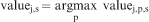dest(j,s) for block j in simulation s can then be determined as the destination that generates the maximum profit or minimum loss, i.e. While the previously outlined method for generating block values, hence destinations, is common in most mine design software for generating pushback designs, there are more advanced methods that should be considered in the future. Generally, the conventional framework for pushback design that the majority of mine planning software currently uses in the industry needs to be reversed: the pushback designs should be generated using a production schedule, given that the production schedule better represents the time dimension, which impacts the net present value of the mine design and considers the annual production capacity constraints. One example of software that operates in this manner is BHP Billiton's Blasor (Stone et al., 2007), which is not commercially available. However, in the proposed framework, this modern methodology is computationally intensive given that the pushback design and production schedule would need to be solved simultaneously. As a result, the proposed methodology is best suited for a conventional framework that generates pushbacks before production scheduling.

Solution shifting

A shift of the solution vector is a perturbation of the pushback design; a central block j is randomly selected, and if it is a candidate for shifting the block from pushback t to t′, the block is then permitted to be tested according to the accept or reject criterion of the simulated annealing algorithm (Algorithm 1).

The ability for a candidate block to be shifted to a different pushback is based on the directly adjacent blocks and the number of predecessors or successors (overlying or underlying blocks, respectively) that need to be corrected to ensure that the slope constraints are respected. Consider a randomly selected block j from Algorithm 1 that needs to be checked if it is a suitable candidate for shifting. Let (i, j, k) denote the coordinates (IJK coordinate system) of block j, and let (ρ(j) denote the list of blocks that need to be corrected to guarantee slope stability. Additionally, consider the minimal sets P(m) and S(m) of predecessors or successors respectively, for any block m and can be calculated with variable slope angles; see Khalokakaie et al. (2000) for a description of the algorithm to generate variable predecessor sets. Algorithm 2 is used to verify whether or not the block is a suitable candidate for shifting. The algorithm uses a breadth-first-search (BFS) algorithm (Cormen et al., 2009) to explore the predecessors or successors that may need fixing up; if there are too many corrections that need to be made (greater than or equal to totFixups), the algorithm stops exploring j and attempts to find another candidate block. The reason for quitting after totFixups corrections is that Algorithm 2 is the bottleneck for the simulated annealing algorithm's performance, and allowing the algorithm to continue the BFS substantially increases the algorithm's running time. It has been shown experimentally that it is sometimes useful to allow the user to set totFixups = ∞, which is referred to as an aggressive shifting strategy, as it can often help the algorithm get out of local optima faster. It is noted that the BFS algorithm uses a queue data structure, where the predecessors or successors are explored in a first-in-first-out (FIFO) manner using generic ‘Enqueue’ and ‘Dequeue’ functions (Cormen et al., 2009). The algorithm either terminates prematurely and states that the randomly selected block j is not a candidate for shifting, or approves the candidate block and returns a set of blocks that need to be shifted to pushback t′ to guarantee slope stability.

Algorithm 2: Check if block is a candidate for solution shift

Initialisation

j, the central block to be considered for shifting the current solution from pushback x_j = t to x_j = t′

, the set of blocks that need to be shifted in order to guarantee slope stability

(i, j, k), the coordinates of the central block j and x((i, j, k)) = t* is the pushback which the block with IJK coordinates (i, j, k) is mined in

true

Algorithm

if x((i, j, k−1)) = x((i, j, k+1)) then

The underlying and overlying blocks are mined in the same pushback, so the current block is not a candidate.

false

return isCandidate

end if

if x((i+1, j, k)) = x(j) and x((i−1, j, k)) = x(j) and x((i, j+1, k)) = x(j) and x((i, j−1, k)) = x(j) then

The blocks on the same plane directly adjacent to block j are all in the same pushback.

false

return isCandidate

end if

if t′>t then

The successors, or underlying blocks, of j need to be explored for correction.

false

end if

Perform Breadth-First-Search (BFS) on predecessors or successors

for each do

false

end for

Q = Ø

Enqueue (Q, j)

while Q≠Ø do

u = Dequeue (Q)

fixupCount = fixupCount+1

if fixupCount> = totFixups then

‘Too many corrections are required – exit and find a new candidate block.

isCandidate = false

return isCandidate

end if

Adj(u) = Ø

if searchUp = true then

Adj(u) = P(u)

else

Adj(u) = S(u)

end if

for each do

if v.explored = false then

v.explored = true

if searchUp = true and x_v>t′ then

Enqueue (Q,v)

else if searchUp = false and x_v<t′ then

Enqueue (Q,v)

end if

end for

end while

return isCandidate and ρ(j)

Application at Escondida Norte Mine, Chile

The two proposed formulations for modifying pushback designs to simultaneously account for grade and material type uncertainty are tested at BHP Billiton's Escondida Norte mine, Chile.

Overview of Escondida Norte Mine

The Escondida mining operation is currently the world's largest open pit copper producer, located 170 km southeast of Antofagasta in northern Chile. For this case study, only a portion of the Escondida mining complex is being considered, called Escondida Norte, which contains ∼176 000 blocks that are 25×25×15 m³ in the x-, y- and z-directions respectively. The mine has provided 50 conditional simulations that contain simulated copper grades, recoveries, tonnage and five simulated material types; the material types are classified as waste, sulphides (low or high recovery), mixed and oxides. Escondida Norte has already mined or is in the process of mining the first two pushbacks (out of a total of 10); this study tests the proposed formulations on the remaining pushbacks (nos. 3–10), and will herein refer to these pushbacks as nos. 1–8. The geological simulations, which contain simulated copper grades and material types, also specify four zones that represent areas that have separate slope angles. In particular, the slopes are set as 33, 35, 41 and 35° for the first, second, third and fourth zones respectively.

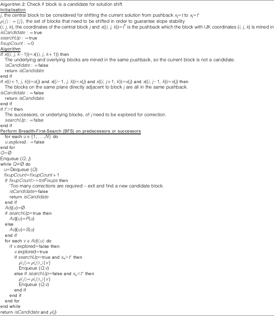
Escondida Norte is capable of extracting a total of 500 000 tonnes per day (500 ktpd); of which the waste goes directly to the waste dump (unlimited capacity), the sulphides have the option to go to one of two mills (both having a capacity of 60 ktpd) or the bioleach pad (unlimited capacity), the mixed ore can go to the bioleach pad, and finally the oxide material can go to the acid leach plant (60 ktpd). Figure 1 shows a flow chart for the potential destinations that each material can be sent to. The copper recoveries for each of the processes are specified for each block in each simulation, and were provided by the mine. The material types (which affect candidate destinations) are also simulated variables, which are specified in the geological simulations. Given that both the Escondida and Escondida Norte mines feed the two mills, the geological simulations show similar recoveries for both mills and the material codes do not distinguish between the two mills, the case study is simplified such that the Escondida Norte material only goes to one of the mills; it is not expected that this decision will have a significant impact on the case study given that the recoveries are similar, and provides a simpler analysis of the algorithm's optimisation performance.

Figure 1

Flow chart of materials to various destinations at Escondida Norte mining operation

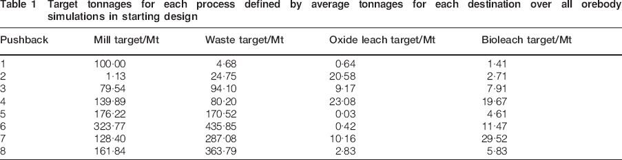
It is assumed that the copper selling price is $1·90/lb, with a selling cost of $0·2/lb. The base mining cost is $1·40/t, with a depth based mining cost adjustment factor applied and is specified in the geological models. The milling, bioleach and oxide leach costs are assumed to be $5·50/t, $1·75/t and $4·25/t respectively. Table 1 shows the target tonnages for each pushback and process from the original design that the annealing algorithm tries to maintain (while simultaneously reducing the variability). It is noted that the target tonnages have all been scaled proportionately.

Table 1

Target tonnages for each process defined by average tonnages for each destination over all orebody simulations in starting design

Pushback	Mill target/Mt	Waste target/Mt	Oxide leach target/Mt	Bioleach target/Mt
1	100·00	4·68	0·64	1·41
2	1·13	24·75	20·58	2·71
3	79·54	94·10	9·17	7·91
4	139·89	80·20	23·08	19·67
5	176·22	170·52	0·03	4·61
6	323·77	435·85	0·42	11·47
7	128·40	287·08	10·16	29·52
8	161·84	363·79	2·83	5·83

Numerical results and analysis

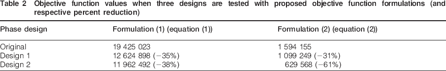
Both proposed formulations are tested on a set of 20 geological simulations. In terms of change in objective function values (evaluating the objective functions proposed in equations (1) and (2) before and after modifying the pushback designs), formulation (1) indicates a decrease of 35% and formulation (2) indicates a decrease of 61%. In both cases, it takes ∼1·5 h to obtain a solution on an Intel i7 2·66 GHz MacBook Pro with 8GB RAM; it is noted, however, that it takes <30 min to converge on a pushback design within 10% of the final solution. Table 2 shows how the three designs (original and two designs from the proposed formulations) perform when evaluating using the proposed objective functions (equations (1) and (2)). When considering formulation (1), described by equation (1), the annealed design that was optimised using formulation (1) (Design 1) reduces the original objective function value by 35%. Interestingly enough, when Design 2 (generated by annealing with formulation (2)) is tested using equation (1), the resulting decrease in objective function value is higher than Design 1, indicating that formulation (2) is outperforming formulation (1); this is likely caused by its ability to better handle variability with its square term. When the designs are evaluated using equation (2), as previously mentioned, Design 2 (generated by annealing with formulation (2)) reduces the initial objective function value by ∼61%. Design 1 does not perform nearly as well under equation (2), and only reduces the objective function value in equation (2) by 31%. This is largely caused by the fact that formulation #1 does not consider the differences in sizes between the pushbacks. This indicates that the design generated by formulation (2) outperforms formulation (1) for either objective function equation, and thus provides better designs, in terms of risk reduction.

Table 2

Objective function values when three designs are tested with proposed objective function formulations (and respective percent reduction)

Phase design	Formulation (1) (equation (1))	Formulation (2) (equation (2))
Original	19 425 023	1 594 155
Design 1	12 624 898 (−35%)	1 099 249 (−31%)
Design 2	11 962 492 (−38%)	629 568 (−61%)

Given that the tonnages going to each of the destinations can vary significantly between pushbacks (e.g. mill tonnage in pushback no. 2), the following analysis has been standardised in terms of the target quantities of materials for each destination and each pushback to provide a clear view of the changes in the risk profile, i.e. for any destination d, pushback p and simulation s, the standardised risk for simulation s is defined as (5) For this analysis, the risk profiles are defined by the minimum and maximum standardised risk (equation (5)) over the simulations for each destination and each pushback; while separating the risk profiles into three graphs for each design and showing the risk profiles for all simulations may lead to a better understanding of the differences in performance between the two algorithms, comparing the minimum and maximum standardised risk values on a single graph is much more clear. It is noted that in the standardised graph, the target value is 1·0 (on the vertical axis); a standardised risk value of 1·6, for example, indicates that one simulation has the potential to have 60% more tonnage than the target indicated in Table 1. Similarly, a value of 0·4 indicates the potential to have 40% less tonnage than the target indicated in Table 1.

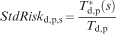
Figure 2 shows the standardised mill tonnage risk profiles for the original pushback design, and the designs after using formulations (1) and (2). Both proposed formulations are able to substantially decrease the minimum and maximum risk in the second pushback when compared to the original pushback design, however it is noted that the mill tonnage in pushback no. 2 is substantially smaller than the other pushbacks, hence would not likely have a significant impact on the mine's operations. Both proposed formulations are able to reduce the downside risk (tonnage below the target) in pushback nos. 3–7 from the original design, which all have large mill tonnages and thus the reduction in risk is likely to have operational significance. In general, both formulations perform very similar in terms of reducing the minimum and maximum risk of the pushback designs, with some improvements from formulation (2) over formulation (1) in pushback no. 2.

Figure 2

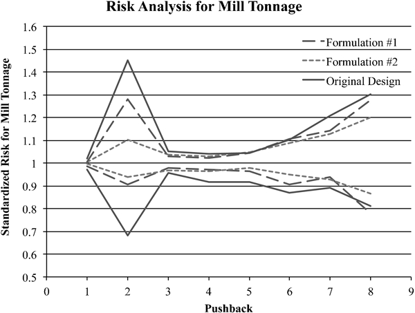
Standardised risk analysis for mill tonnage in original, formulations (1) and (2) designs

Figure 3 shows the risk profiles for the waste tonnage for each pushback. It can be seen that the original design has a substantial amount of risk in waste tonnage for the first pushback; both formulations (1) and (2) substantially reduce this standardised risk from approximately ±50% to (+29%/−15%) and ±8% respectively. This risk, however, is associated with a small target waste tonnage, hence the reduction in variability is not expected to have any operational significance. Figure 3 also indicates a reduction in the downside risk (standardised risk for waste tonnages greater than 1) from both formulations by ∼10% for pushback nos. 4–7, which confirms the result of reducing the downside risk in mill tonnage in Fig. 2. It is clear that once again, the difference in the performance between the two proposed objective function formulations is almost negligible for the minimum and maximum standardised risk values. There is a slight improvement for the minimum and maximum standardised risk profiles by formulation 2 in the final three pushbacks, however it is not significant.

Figure 3

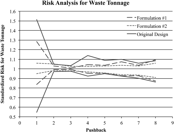
Risk analysis for waste tonnage in original, formulations (1) and (2) designs: note that waste tonnages have been standardised to original design's target size

Figure 4 shows the standardised risk profiles for the tonnage sent to the oxide (acid) leach process. All three designs show similar standardised risk profiles, with the exception of pushback no. 5, where the original design shows a drastic amount of risk in tonnage. Formulation (1)'s standardised risk profile for pushback no. 5 shows an increase in risk, whereas formulation (2) shows a drastic reduction in risk. It is noted, however, that the total tonnage sent to the acid leach process in pushback no. 5 amounts to ∼2 days of the mine's production, and this variability is therefore not expected to have a drastic effect on the mine's overall value.

Figure 4

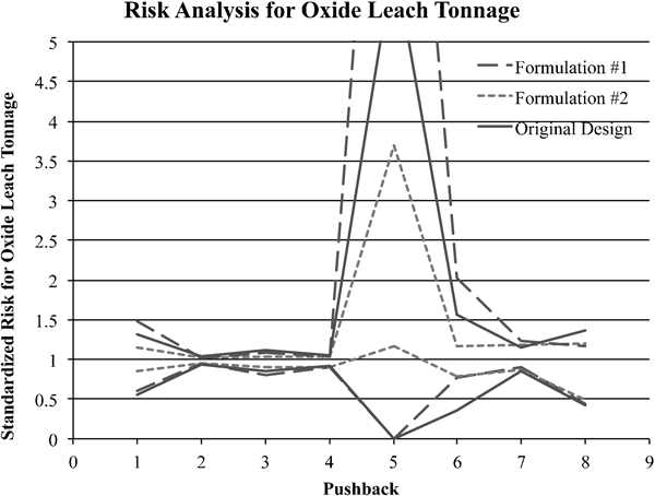
Standardised risk analysis for oxide tonnage in original, formulations (1) and (2) designs

Figure 5 shows the standardised risk profiles for bioleach tonnage. In this case, there is a clear difference between the two methods; formulation (1) does not appear to obey the target tonnages, which is likely a result of the fact that the target sizes for the bioleach process are smaller than the mill and the optimiser is reducing the overall risk of the design by shifting it to the bioleach process; this is a perfect example for why formulation (2) was proposed. Formulation (2) generates entirely different risk profiles that lead to higher quantities of mixed (bioleach) material mined in the first and third pushbacks, and reduced quantities mined in the fifth and eighth pushbacks. Overall, it appears that formulation (2) was able to reduce the risk in the bioleach tonnage over the original design; while the profiles may appear to fluctuate around different means, the difference between the minimum and maximum curves is smaller for this design. This is not a significant change given that the quantities of mixed material in these pushbacks are low compared to the other pushbacks.

Figure 5

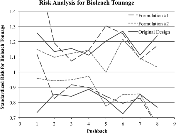
Standardised risk analysis for bioleach tonnage in original, formulations (1) and (2) designs

Table 3 shows the total undiscounted cash value for each of the pushbacks for the three designs; it is noted that the cash values have been scaled arbitrarily and do not reflect reality. Both designs that result from the two proposed formulations have 7–10% higher undiscounted value in the first pushback than the original design. This difference is recovered by the original design in pushback no. 3, however both formulations show a 10–12% increase in value for the fourth pushback over the original design. By moving the undiscounted cash values forward through the life of the mine, the designs generated by the proposed formulations may lead to an increased net present value after production scheduling is performed because discounting will favour the higher valued pushbacks mined early in the mine's life; however, these assumptions will need to be confirmed with stochastic LOM production scheduling. Given that a fair comparison between the deterministic and stochastic mine design frameworks would require a substantial amount of detail regarding long term production scheduling (e.g. Albor and Dimitrakopoulos, 2010), this comparison is will be a topic of future research.

Table 3

Average undiscounted cash values for each pushback for starting designs and designs after applying proposed formulations (values have been scaled)

Pushback	Average undiscounted value
Pushback	Starting design ($ million)	Formulation (1) design ($ million)	Formulation (2) design ($ million)
1	100	106·6	109·82
2	16·37	17·26	17·91
3	66·72	65·19	58·74
4	98·42	107·78	110·28
5	78·65	77·74	80·27
6	131·32	119·00	116·44
7	45·64	46·63	49·12
8	39·12	36·04	33·66

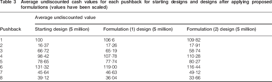
Figure 6 shows the risk analysis of undiscounted values, where the values are standardised in terms of the design's own average undiscounted value (rather than in terms of the original design used for standardised risk analysis of tonnages). For pushback nos. 1–3, the differences between risk profiles for all three designs are negligible, however the differences are more pronounced for the later pushbacks, where the proposed formulations show substantially less risk than the original design, in the order of 10–20%. This is a result of reducing the risk for the mill and waste tonnages for pushbacks nos. 4–7 discussed previously.

Figure 6

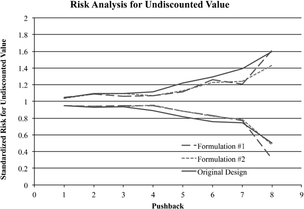
Standardised risk analysis for undiscounted cash values for original pushback design and formulations (1) and (2)

The undiscounted value risk profile for the original design performs extremely well; in specific, there is very little risk in the first pushbacks, and grows gradually for the remaining pushbacks; this result is generally not expected, given that conventional mine design frameworks do not understand uncertainty that is represented through a set of geological simulations, and thus do not understand the effects of deferring it to later pushbacks (or production periods). Using a conventional framework, it is expected that the risk profiles are substantially more erratic than what is shown in Fig. 6 because there is no control over the uncertainty. In order to incorporate this risk-deferral of undiscounted cash flows in any of the proposed formulations, one can simply add a penalty cost to the variance of undiscounted cash flows, where the penalty cost is reduced for each subsequent pushback. Similar concepts are used for production scheduling under uncertainty with stochastic integer programming (Dimitrakopoulos and Ramazan, 2008; Ramazan and Dimitrakopoulos, 2012).

Figure 7 shows a sample cross-section from the original pushback design, and the sections from the resulting pushback designs from formulations (1) and (2). While there are some consistencies in terms of the locations of the pushbacks, the algorithm seems to have chosen pushback designs that are similar to the type of pit shells commonly seen with conventional mathematical optimisation tools. It can be seen that the first four remain relatively unchanged, which is indicative of lower uncertainty near the surface. It is apparent that the algorithm is still respecting the various slope angles, and has changed the initial design considerably to be able to attain the reductions in risk that were previously discussed.

Figure 7

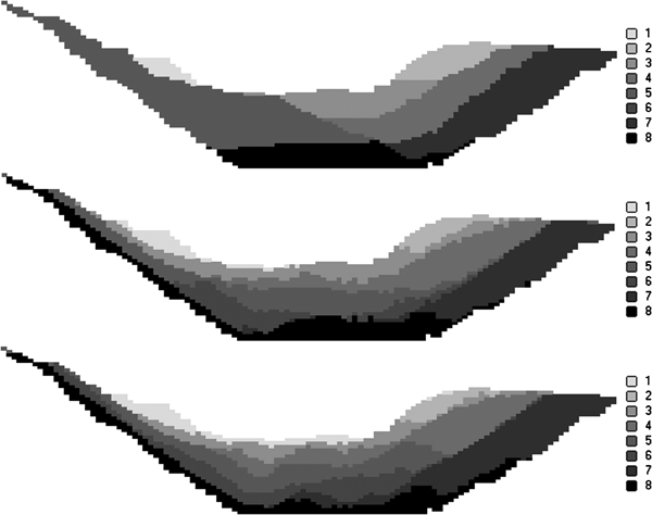
Cross-sections of pushback designs: i: original design; ii: formulation (1) design; iii: formulation (2) design

Conclusions

This paper proposes two general formulations to modify an existing pushback design to incorporate joint local geological uncertainty and is implemented using a simulated annealing algorithm. The proposed formulations and algorithm contributes and improves on existing stochastic mine design frameworks because it can accommodate joint uncertainty between multiple metals and material types and multiple material destinations; and directly reduces the geological risk associated with pushback designs for each material destination. The proposed formulations and implementation can be easily integrated into any existing framework used by a mine to aid in minimising the variability of materials, be it a deterministic or stochastic framework. The proposed algorithm using simulated annealing is computationally efficient and suitable for real world applications because it is capable of considering multiple metals, materials, destinations and slope zones.

The proposed formulations are tested on BHP Billiton's Escondida Norte mine, Chile. The two proposed formulations often show significant reduction in variability for pushbacks that are particularly problematic, without displacing the risk to other material destinations or pushbacks. The second proposed objective function formulation outperformed the first formulation in this case study, with an overall reduction in objective function by 61% over the original design; additionally, the second design also outperforms the first design when evaluated with the first objective function by an additional 3%. This is a result of its ability to better penalise variability using a squared deviation from target, along with the fact that it treats all processes equally, regardless of the tonnages going to the various processes. While the proposed designs appear to have higher values and reduced risk in the earlier pushbacks, the true effects on the net present value of the proposed pushback design methodology would need to be tested with long term production scheduling.

Future work will seek to integrate the proposed pushback design algorithms with stochastic LOM production scheduling, and quantify the impact that stochastic pushback design has on the annual production schedules. Additionally, new methods for pushback design need to be developed for industrial use. These production schedules should, unlike the conventional approaches, integrate uncertainty and consider the pushback design's direct influence on the net present value and annual capacity constraints. However, this type of a development will require substantial enhancement of computational efficiency of the related scheduling methods.

Footnotes

Acknowledgements

The work in this paper was funded from the National Science and Engineering Research Council of Canada, Collaborative R&D Grant CRDPJ 411270-10 with AngloGold Ashanti, Barrick Gold, BHP Billiton, De Beers, Newmont Mining, and Vale. Thanks are in order to Brian Baird of BHP Billiton for his support, collaboration, and technical comments.

Appendix

This paper is part of a special issue on Strategic Mine Planning

References

Albor Consuegra

, Dimitrakopoulos

2009. Stochastic mine design optimisation based on simulated annealing: pit limits, production schedules, multiple orebody scenarios and sensitivity analysis, Min. Technol. (Trans. Inst. Min. Metall. A), 118, (2), A80–A91.

Albor Consuegra

, Dimitrakopoulos

2010. Algorithmic approach to pushback design based on stochastic programming: method, application and comparisons, Min. Technol. (Trans. Inst. Min. Metall. A), 119, (2), A88–A101.

Asad

MWA

, Dimitrakopoulos

2012. Implementing a parametric maximum flow algorithm for optimal open pit mine design under uncertain supply and demand, J. Oper. Res. Soc., published online ahead of print, doi 10.1057/jors.2012.26.

Boucher

, Dimitrakopoulos

2009. Block simulation of multiple correlated variables, Math. Geosci., 41, (2), 215–237.

Cormen

, Leiserson

, Rivest

. 2009. ‘Introduction to algorithms’, 594–601; Cambridge, MIT Press.

Dagdelen

2007. Open pit optimization – strategies for improving economics of mining projects through mine planning. Orebody Modelling and Strategic Mine Planning Spectrum Series, 14, (, Dimitrakopoulos

), 145–148; Victoria, The Australasian Institute of Mining and Metallurgy.

Dimitrakopoulos

, Farrelly

, Godoy

2002. Moving forward from traditional optimization: grade uncertainty and risk effects in open pit design, Min. Technol. (Trans. Inst. Min. Metall. A), 111, (1), A82–A88.

Dimitrakopoulos

, Ramazan

2008. Stochastic integer programming for optimizing long-term production schedules of open pit mines: methods, application and value of stochastic solutions, Min. Technol. (Trans. Inst. Min. Metall. A), 117, (4), A155–A160.

Geman

, Geman

1984. Stochastic relaxation, Gibbs distribution, and the Bayesian restoration of images, IEEE Trans. Patt. Anal. Mach. Intell., (6), 721–741.

10.

Godoy

2003. The effective management of geological risk in long-term production scheduling of open pit mines, PhD thesis (unpublished), University of Queensland, Brisbane, Qld, Australia.

11.

Hochbaum

, Chen

2000. Performance analysis and best implementations of old and new algorithms for the open-pit mining problem, Oper. Res., 48, (6), 894–914.

12.

Hustrulid

, Kuchta

2006. Open pit mine planning and design, 482–640; Rotterdam, A.A. Balkema.

13.

Journel

, Huijbregts

. 1978. Mining geostatistics, 53–74; London, Academic Press.

14.

Khalokakaie

, Dowd

, Fowell

. 2000. Lerchs-Grossmann algorithm with variable slope angles, Min. Technol. (Trans. Inst. Min. Metall. A), 109, (2), A77–A85.

15.

Kirkpatrick

, Gelatt

, Vecchi

1983. Optimization by stimulated annealing, Science, 220, (4598), 671–680.

16.

Leite

, Dimitrakopoulos

2007. Stochastic optimization model for open pit mine planning: application and risk analysis at a copper deposit, Min. Technol. (Trans. Inst. Min. Metall. A), 116, (3), A109–A118.

17.

Lerchs

, Grossmann

. 1965. Optimum design of open pit mines, Trans. CIM, 67, 17–24.

18.

Meagher

, Abdel Sabour

, Dimitrakopoulos

2010. Pushback design of open pit mines under geological and market uncertainty, Proc. Orebody Modelling and Strategic Mine Planning Spectrum Series, 17 (, Dimitrakopoulos

), 291–298; Burwood, The Australasian Institute of Mining and Metallurgy.

19.

Picard

. 1976. Maximal closure of a graph and applications to combinatorial problems, Manag. Sci., 22, (11), 1268–1272.

20.

Ramazan

, Dimitrakopoulos

2012. Production scheduling with uncertain supply: a new solution to the open pit mining problem, Optim. Eng., published online ahead of print, doi 10.1007/s11081-012-9186-2.

21.

Rondon

2012. Teaching aid: minimum/maximum autocorrelation factors for joint simulation of attributes, Mathe. Geosci., 44, (4), 469–504.

22.

Stone

, Froyland

, Menabde

, Law

, Pasyar

, Monkhouse

PHL

. 2007. Blasor – blended iron ore mine planning optimisation at Yandi, Western Australia, Proc. Orebody Modelling and Strategic Mine Planning Spectrum Series, 14, (, Dimitrakopoulos

), 133–136; Burwood, The Australasian Institute of Mining and Metallurgy.

23.

Strebelle

2002. Conditional simulation of complex geological structures using multiple-point statistics, Math. Geol., 34, (1), 1–21.

24.

Tachefine

, Soumis

1997. Maximal closure on a graph with resource constraints, Comput. Oper. Res., 24, (10), 981–990.

25.

Whittle

1988. Beyond optimisation in open pit design, Proc. Computer Applications in the Mineral Industries, (, Fytas

), 331–337; Rotterdam, A.A. Balkema.

Algorithmic integration of geological uncertainty in pushback designs for complex multiprocess open pit mines

Abstract

Keywords

Introduction

Modifying pushback designs to manage geological uncertainty

Formulations for modifying starting design

Formulation (1)

Formulation (2)

Implementation using simulated annealing

Simulated annealing algorithm

Block destinations

Solution shifting

Application at Escondida Norte Mine, Chile

Overview of Escondida Norte Mine

Numerical results and analysis

Conclusions

Footnotes

Acknowledgements

Appendix

References