
Abstract
This paper investigates the financial and environmental consequences stemming from the introduction of a carbon levy applied to mining and processing activities. The novelty is twofold: (1) the effect of a carbon tax, proportional to the emissions produced by all relevant mining activities, is accounted for in the determination of the Ultimate Pit Limit (UPL), i.e. the environmental costs are not applied a posteriori to pit optimization but included concurrently to Net Present Value (NPV) maximization, allowing to investigate the relationship between carbon tax value versus NPV, amount of ore extracted and carbon emissions; (2) we use a new software, OptimalSlope, to automatically determine geotechnically optimal profiles for the mine pitwalls. The Marvin copper deposit (block model data publicly available from MineLib repository) was adopted as a case study. Several pit optimizations were performed based on four different values of carbon tax and adopting either traditional planar or non-linear optimal pitwalls. It emerges that the relationships between carbon tax value versus NPV, amount of ore extracted, and carbon emissions exhibited linearity in both cases of planar and optimal pitwall profiles. Moreover, the adoption of optimal profiles realizes gains up to 215 million AUD, without compromising the safety of the UPL.
Keywords
Introduction
Among human industries and activities, mining is possibly one of the most energy and carbon-intensive (Igogo et al. 2021). At the 26th United Nations Climate Change Conference (COP26), miners were challenged to make commitments to align with the target of achieving net-zero carbon dioxide emissions by 2050. Between the several important issues, investing in greener operation methods and emission reduction technologies was identified as increasingly important across the entire sector.
It is recognized by most that mining of metals is necessary for the transition towards renewables and more sustainable transportation systems (e.g. electric vehicles) with the demand for many metals forecast to grow in the decade as a result of the transition to renewables (Månberger and Stenqvist 2018). For instance, according to the World Energy Outlook Sustainable Development Scenario, clean energy technologies will need over 40% more copper and rare earth elements, 60-70% more nickel and cobalt, and almost 90% more lithium by 2040 (IEA 2021). Potential substitutes for metal use are often inadequate or simply do not to exist at present (Graedel et al. 2015). Hence, in the face of increasing demand and decreasing mineral ore grade (Norgate and Haque 2010; Lezak et al. 2019), prices for rare earth minerals are predicted to increase with a growth of energy demand as much as 36% by 2035 (Maennling and Toledano 2018). Consequently, innovative solutions are urgently required to reduce mining environmental impacts while at the same time preserving profitability of projects to ensure mining remains a viable business providing the minerals needed to make it possible to achieve the net zero targets of many governments.
Carbon pricing or carbon levy is an instrument increasingly considered by governments to incentivise decarbonization of industrial activities and to capture the cost of environmental degradation due to greenhouse gas emissions (GHG). It is also considered a tool to make polluters pay. The advantage of this tool over more blunt instruments like mandating carbon caps is that no hard limits on emissions are prescribed, but instead a carbon levy is set to incentive emitters to reduce emissions progressively over time allowing themselves to plan the extent to which they can afford to adjust their activities and the pace of the adjustments in the face of the price to be paid. Moreover, the money raised by the levy can be used by governments to subsidise green technologies and policies, setting up a virtuous circle of change. Carbon pricing mechanisms (The World Bank 2021) are subdivided into explicit, implicit, and internal carbon pricing. The first includes policies introduced by governments imposing a price based on carbon content, such as carbon taxes or Emission Trading Systems (ETS). The second involves policies that theoretically derive an implicit carbon price by calculating the equivalent monetary value per tonne of carbon associated with a specific policy instrument. However, estimating implicit carbon costs of policy instruments necessitates a quantitative method, which can be difficult in many circumstances.
Muñoz et al. (2014) presented a methodology to calculate equivalent carbon emissions and energy use due to the main mining activities at the Block Model (BM) level. In this paper, a novel methodology will be introduced to include the carbon tax which is proportional to the amount of emission produced as additional costs for each block of the mine BM with the cost accounting for the emissions produced by all the emitting mining activities. This enables accounting for the economic effect of the carbon tax on mine profitability in the determination of the UPL and pushbacks which are then determined in the usual way via a single objective function based on NPV maximization. Therefore, a key advantage over previous attempts to include environmental aspects in pit mine design, e.g. Pell et al. (2019), is the fact that environmental costs are not applied a posteriori to pit optimization but included concurrently so that the sequence of pushbacks produced as a result of the mine design is financially optimal for the specified carbon tax prescribed. Additionally, to quantify the benefits of this approach, we compare the NPVs resulting from this approach to the ones obtained applying the carbon tax after the end of the pit optimization phase.
Pitwall inclination has a massive effect on mine environmental impact and profitability since it controls to a large extent the amount of rockwaste to be excavated (Hustrulid et al. 2013). Moreover, between 1930 and 2000, the depth of the average discovery in Australia, Canada, and the United States increased from surface outcropping to 295 m (Randolph 2011). Consequently, ensuring pitwalls are as steep as possible has grown in importance. Evidence that slope profiles non-linear in cross-section, i.e. a profile whose inclination varies with depth, are better than linear ones was first reported as far back as 1890 (Newman 1890). The author observed that cuttings of concave shape excavated in homogeneous clay layers tended to be more stable than planar ones with the same Overall Slope Angle (OSA), which are more stable than cuttings of convex shape. Almost a century later, Hoek & Bray, in chapter 12 of the second edition of Rock slope engineering (Hoek and Bray 1977), analysed the stability of some concave circular slopes in cross-section. They found the stability number, a dimensionless index capturing the mechanical stability of a slope introduced by Taylor (1937), for circular profiles to be higher than their planar counterparts, i.e. the planar slopes with the same OSA, which share the same toe and crest points. After that, the first systematic theoretical study on the mechanical properties of concave slope profiles for geomaterials exhibiting some cohesion, so applicable to all rocks and clayey soils, appeared in Utili and Nova (2007). By employing the upper bound theorem of limit analysis, Utili & Nova proved that logspiral profiles exhibit higher Factor of Safety (FoS) than their planar counterparts for any value of c and φ considered with the highest gain for inclinations midway  and the vertical line, i.e. for
  . Later, other researchers (Jeldes et al. 2015; Vahedifard et al. 2016; Vo and Russell 2017) have independently investigated the stability of concave profiles excavated in uniform slopes. They all employed different methods for assessing slope stability: the slip line method, limit equilibrium methods, and the finite element method. However, they all reached the same conclusion concerning the superior stability of non-linear (concave) profiles. Nevertheless, a fundamental limitation of the studies listed above is the assumption that the shape claimed to be optimal is found as the shape associated with the highest stability number among curves belonging to a very restricted family and the assumption of uniform slope. More recently, Agosti et al. (2021a, 2021b) and Utili et al. (2022) employed a novel geotechnical software, OptimalSlope (Utili 2016), that computes the slope optimal profile for any specified lithological sequence without unduly restricting the search to any predefined family of shapes to design the pitwalls of three open pit mines achieving important increases of NPV and carbon footprint reductions in comparison with the traditional design based on planar pitwalls. To be able to quantify the gains of NPV and carbon footprint reduction in a consistent way in Agosti et al. (2021b, 2021a) and Utili et al. (2022) the open pit mines considered were designed twice employing the same pit optimizer software, economic parameters and optimization strategy, with the only difference between the two designs being the pitwall profiles adopted. Financial and environmental gains were calculated as the difference between the NPV, carbon footprint and energy consumptions resulting from the two designs. Also in this paper, the same pit design methodology is used and both traditional and optimal pitwall profiles are considered.
In the following, first the Marvin case study is presented (Section 2); second the open pit mine design methodology is illustrated including the implementation of the carbon levy into pit optimization (with carbon levy considered at the BM level and concurrently to pit optimization); third the results of various designs for different levels of carbon tax with either traditional or optimal pitwall profiles are presented including the relationships illustrating the effect of carbon tax levy on NPV, amount of ore extracted and carbon emissions; fourth conclusions from the emerging trends are presented.
Case study: the Marvin copper deposit
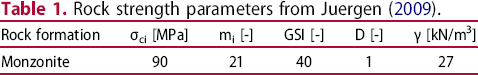
Rock strength parameters from Juergen (2009).
Rock strength parameters from Juergen (2009).
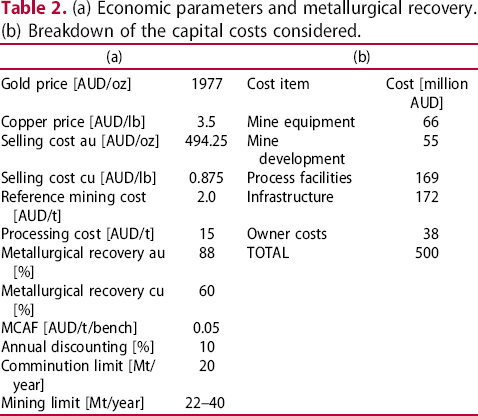
(a) Economic parameters and metallurgical recovery. (b) Breakdown of the capital costs considered.
The iterative procedure employed to calculate the UPL is explained in detail in Utili et al. (2022) and was also employed for the strategic design of other two mines (Agosti et al. 2021b, 2021a). The procedure, which is recalled in Figure 1, is the same irrespective of the shape of the pitwall profile adopted, i.e. planar or optimal profile. At the beginning, an initial pit depth (HUPL,0) was assumed as the depth of the orebody from the topographic surface. Then, we calculated the pitwall profile: in the case of planar pit walls we find, by trial and error, the maximum OSA compatible with the target FoS (with the FoS of each trial profile calculated by Limit Equilibrium using Rocscience Slide2), whereas for optimal pit walls employing OptimalSlope (see Section 3.1). Then, we assigned the calculated pitwall profiles and the relevant economic and metallurgical parameters as an input into the pit optimizer (GEOVIA Whittle) together with the carbon tax by adding block by block the carbon tax as costs which are calculated on the basis of the amount of CO2,eq emitted for all the relevant mining activities (see Section 3.2). Finally, we ran the pit optimizer to produce the UPL and pushbacks (the steps entailed are described in Section 3.2). The UPL depth obtained as an output of the strategic pit optimization, HUPL,1, was then compared to the one prescribed as input in the slope design process, HUPL,0. If it turns out to be different (planar case), a second iteration would be performed with the height HUPL,1 to be used as input for a second slope design process followed by a second run of the pit optimizer. However, only one iteration was necessary in this case study, both for the case of planar and optimal pitwalls. The values of the pit wall height and OSA for each value of carbon tax employed are reported in Section 4.
Flow chart illustrating the iterative process used to determine the ultimate pit limit and pushbacks (modified after Utili et al. (2022)) Note that the process is the same irrespective of the shape of the adopted pitwall profiles. Images are available in colour online.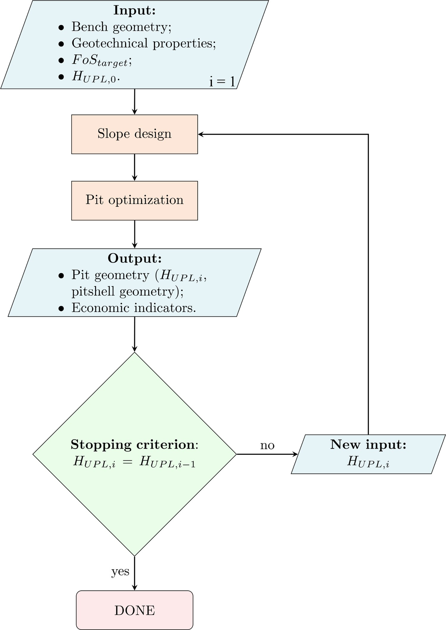
Acceptability criteria.
Acceptability criteria.

Next, we computed the minimum berm width, using the equation proposed by Call (1992) published in the SME Mine Engineering Handbook (Hartman et al. 1992) known as modified Ritchie's criteria, which has been demonstrated to be effective in field tests in several benched mine slopes (Ryan and Pryor 2001) and it is largely used by practitioners as reported in Read and Stacey (2009). The adequacy of the chosen berm widths can be verified via either computer modelling, e.g. Frac_Rock: programme for the analysis of discontinuous rock masses (2016) or analytical equations (Gibson et al. 2006). In Coetsee (2020), a recent extensive review of the bench design methodologies currently employed by the open pit mine industry is provided. Note that the containment of fragments generated by bench excavation and local wedge failures are not necessarily captured by the modified Ritchie formula and may dictate larger bench width values.
Then, we computed the geotechnically optimal slope profiles for the representative cross-section of the mine using the slope optimizer OptimalSlope. The input data required by OptimalSlope are standard geotechnical parameters (rock mass strength and unit weight) together with the geometries of benches (bench height and face inclination) and ramps (see Figure 2) and any overburden or surcharge if present. A detailed explanation of how OptimalSlope works can be found in Utili et al. (2022), therefore it will not be repeated here. In Figure 2 the input and output data are reported.
OptimalSlope Graphical User Interface with data input (screens a; b; c; d; e; f; g; h; i; l; m) and output (screen n). Bench and ramp geometries are requested so that the optimal profile complies with all the geometric constraints stemming from bench design and presence of any ramps. Images are available in colour online.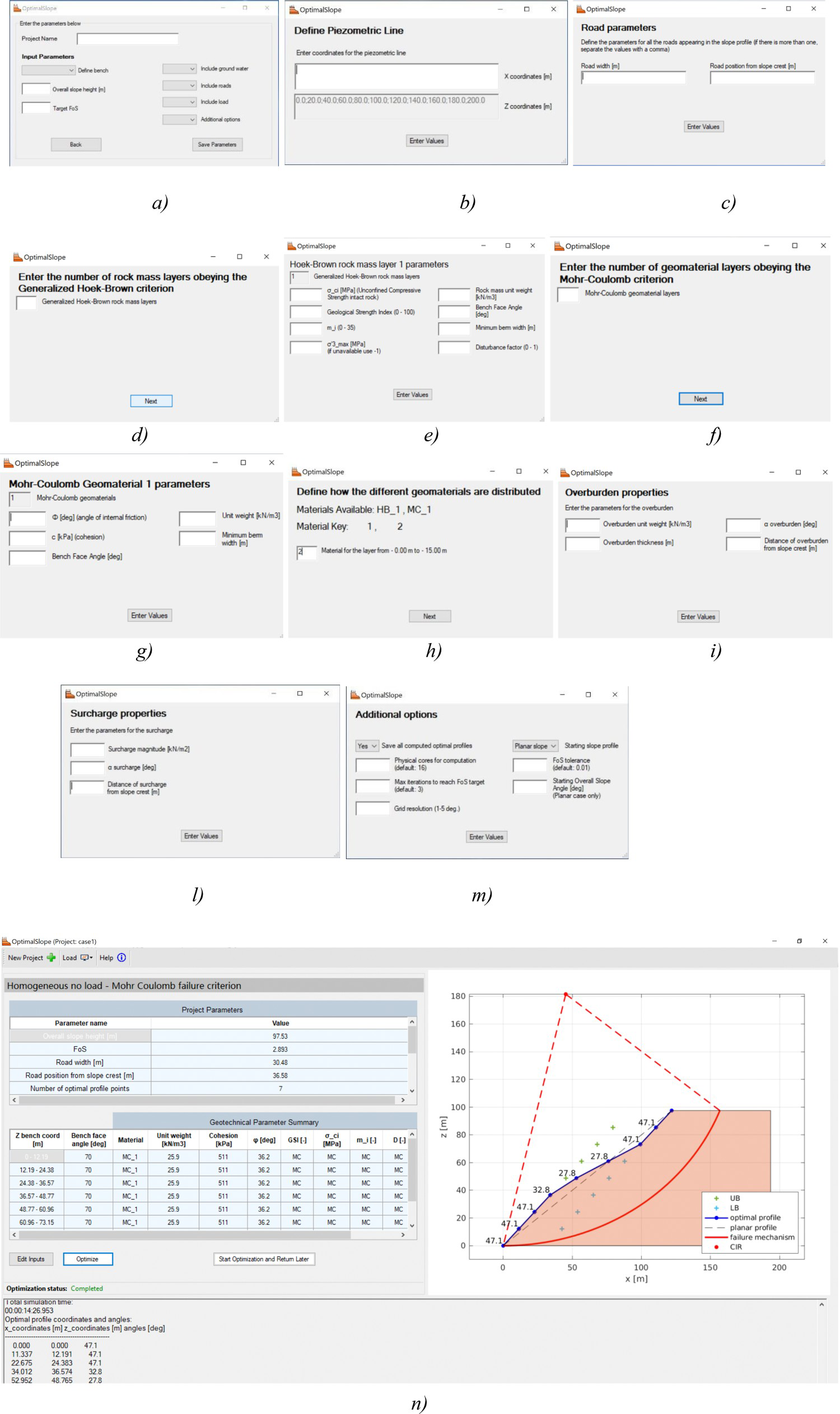
Recently, a few works have appeared in the literature to perform the life cycle assessment of open-pit mines (Ekman Nilsson et al. 2017; Chen et al. 2018; Gan and Griffin 2018).
Muñoz et al. (2014) were the first to conceptualize a methodology to calculate energy consumption and carbon emissions directly into the BM. However, they did not apply their approach on any actual mine, used a bespoke non-commercial pit optimizer without considering the effect of time in their computations (did not calculated NPV but only undiscounted profit) and, very importantly, did not investigate the sensitivity of the costs associated to carbon emissions in their pit optimization. These are all aspects introduced in this paper. Muñoz et al. (2014) identify three main energy consumption stages: mining, concentrating (which in the paper is the combination of crushing and grinding, commonly defined as comminution), and hydrometallurgical. However, the hydrometallurgical stage has not been considered here since Ballantyne et al. (2012) showed this stage to have a negligible effect on energy consumption and emissions in comparison with hauling and comminution.
Recently, Pell et al. (2019) presented an approach where NPV maximization and Global Warming Potential (GWP) minimization are both pursued in strategic mine planning based on a multi-objective function with a weighting factor attributed to NPV maximization and another one to carbon footprint (or energy consumption) minimization. Although certainly a first important step in the direction of including environmental damage minimization in mine strategic planning, this approach suffers from the subjective judgement that mining companies need to make to determine the weighting factors and cannot be used by policymakers since mandating a weighting factor for environmental importance and one for NPV maximization is too ambiguous and prone to manipulation to be legally enforced. Moreover, in Pell et al. (2019), the pit optimization process, i.e. the determination of pushbacks or phases of mine development, is still entirely based on NPV maximization alone without including emission minimization.
Following Muñoz et al. (2014), first we evaluated the energy consumption of each block based on the physical processes taking place, then calculated the GWP from the estimated energy consumption. Our procedure to implement the CO2 tax into the pit optimizer (Geovia Whittle or Datamine Studio NPVS) is illustrated in Figure 3. Note the procedure is the same irrespective of the shape of the pitwall profile adopted, i.e. planar or optimal profile. In the case of Geovia Whittle (2021) (see Figure 3(a)), as a first step, the principal mining operations are subdivided between activities applied to all blocks regardless of their destination and executed only to blocks directed to the waste dump and comminution plant. This subdivision is necessary to correctly implement carbon prices inside the pit optimization process without approximating the carbon emissions and associated costs. In determining the most economic UPL, prices, costs and geotechnical constraints (i.e. the inclination of the pitwalls) entirely dictate the shape of the UPL. Therefore, prior to pit optimization the destination of any block is still undetermined, i.e. a block containing ore may be sent either to the comminution plant, or the waste dump or left in place depending on what turns out to be more profitable. Hence, the amount of carbon emissions due to mining is also unknown.
Flow chart illustrating the methodology employed to implement the CO2 cost into the pit optimiser: (a) for Geovia Whittle; (b) for Datamine Studio NPVS. Images are available in colour online.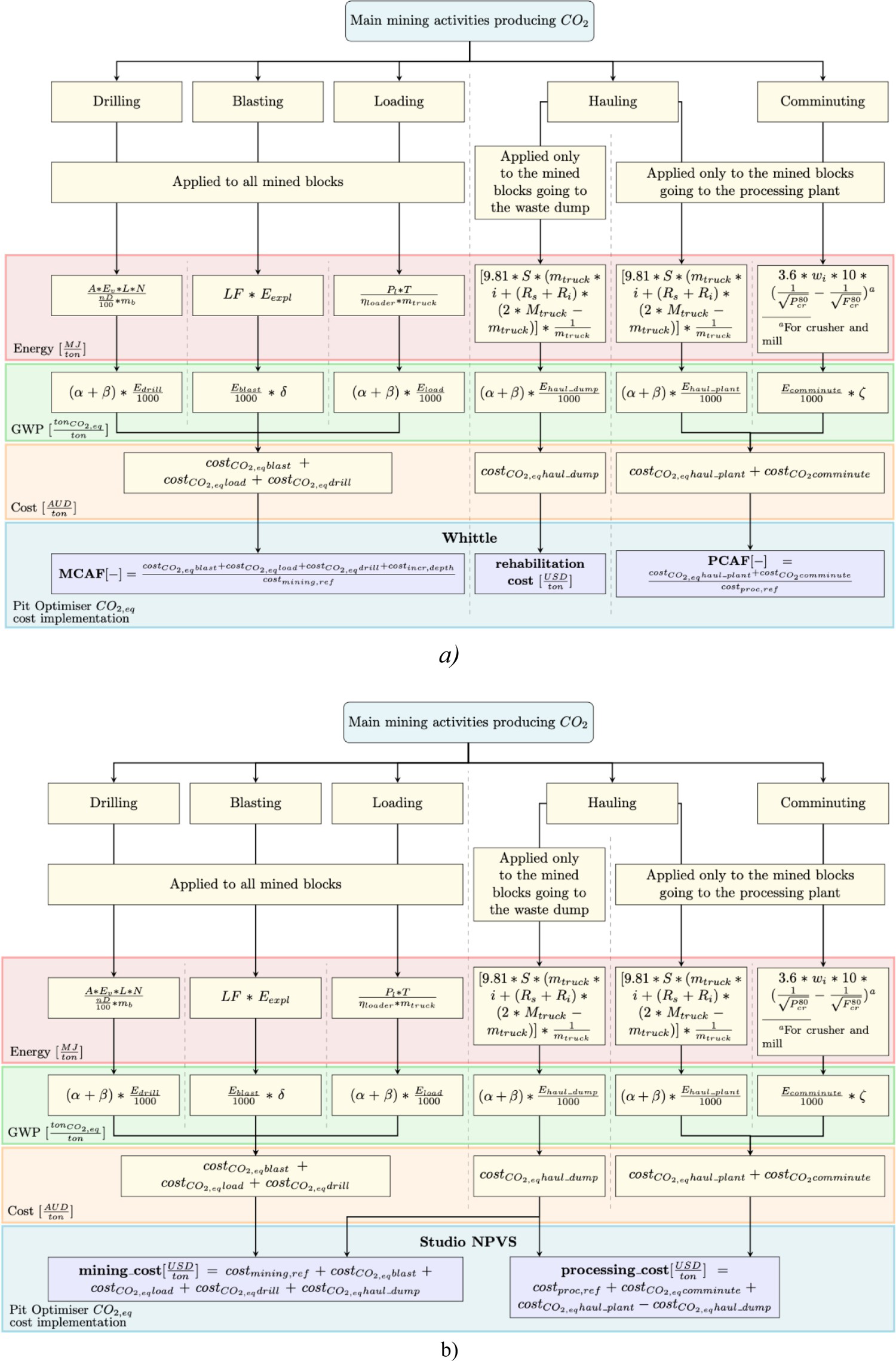
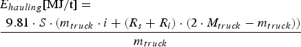
For this reason, we decided to group drilling, blasting, and loading. These three mining activities are performed on every block selected to be extracted by the Lerchs-Grossmann (or Pseudoflow) algorithm. Hauling the mined material out of the pit is undoubtedly a necessary operation producing a large part of the total emission (Ballantyne et al. 2012) which are directly proportional to the distance covered by the dumpers to transport the material to destination (i.e. comminution plant or waste dump). Therefore, we differentiated between emissions related to block transportation to the comminution plant and transportation to the waste dump. Lastly, the comminution stage, which is the process of reducing solid materials from one average particle size to smaller average particle size through the use of crushing, grinding, cutting, vibrating, or other methods (Bond 1952) is performed only on mined material, classified as ore. Therefore, this was applied only to a subset of mined blocks. Then, we calculated the energy required to produce one tonne of mined ore and associated GWP from block properties such as grade, mass, load factor, and block distance to a reference point on the surface using the equations introduced by Muñoz et al. (2014).
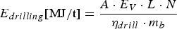
For drilling, the energy consumption is calculated as Muñoz et al. (2014):
 is the number of drill holes for each block; E v
  is the drilling specific energy that depends on rock type and was estimated based on a unified classification system of rocks according to their drillability (Isheyskiy and Sanchidrián 2020);
  is the assumed driller efficiency;
  is the mass of the block in tonnes.
The specific energy that an explosive can deliver when detonated is computed with the formula (Muñoz et al. 2014) :

 is the load factor, defined as the amount of explosive per tonne of detonated rock;
  is the specific explosive energy (Muñoz et al. 2014) for ANFO, the type of explosive here employed.
The specific energy that a front loader consumes to load up the fractured material on the dumper can be computed with the expression (Muñoz et al. 2014):
 is the front loader power (having assumed a CAT 950 GC); T = 45 s is the assumed average time to meet the loading capacity of the dumper using the front loader;
  is the assumed front loader efficiency;
  is the loading capacity of the dumper (having assumed a Komatsu HD 785-8), considering the dumper fully loading at every trip.
 is the inclination of the ramp;
  is the rolling resistance of the surface taken from Soofastaei et al. (2016);
  is the assumed internal resistance of the dumper;
  is the total mass of the loaded dumper (Komatsu HD 785-8).
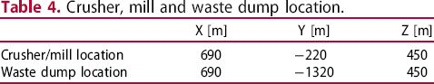
Crusher, mill and waste dump location.
The specific energy to comminute a tonne of ore can be computed with Bond's law (Bond 1952; Muñoz et al. 2014):
 (Bond 1952);
 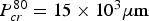 and
and  are the 80% passing sizes of the product for the crusher and the mill;
  and
and  are the 80% passing sizes of the feed for the crusher and the mill.
To calculate the mine carbon footprint, the specific energy consumptions per tonne were translated into specific carbon footprints using characterization factors to include scope 1, 2 and 3 emissions associated with the mining activities by using the following equation (Muñoz et al. 2014):
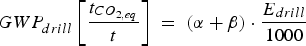
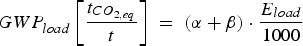

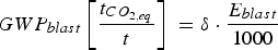
α = 0.09159 β = 0.5200 δ = 2.270 ζ = 0.5646 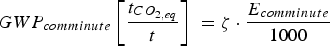
 /MJ;
/MJ; /MJ;
/MJ; /MJ.
/MJ. /kWh.
/kWh.
Then, the specific carbon emissions for each principal mining activity were multiplied by the tonnages of the ith block and the carbon tax value to determine the CO2 cost related to the drilling, blasting, loading, hauling and comminuting.
Finally, the resulting carbon costs were implemented into the pit optimizer following the subdivision introduced above. We implemented the carbon costs into the mining activities for every block selected to be extracted into the block Mining Cost Adjustment Factor (MCAF). While for the mining activities applied only to the blocks selected to be extracted and destined to the comminution plant, we used the block Processing Cost Adjustment Factor (PCAF). MCAF and PCAF are two dimensionless scalars defined on a block-by-block basis with the following expressions:
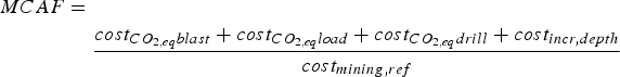
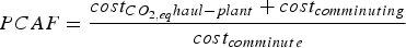
 is the mining reference cost increased by 0.05 AUD/t/bench (see Table 2 a);
  is the reference mining cost (see Table 2 a);
  is the cost related to the carbon emissions for hauling the ore from the pit to the comminution plant;
  is the reference processing cost (see Table 2 a).
Lastly, to account for the carbon cost related to hauling between pit and the waste dump, we employed the so-called ‘rehabilitation cost’ since it is only applied to blocks that are directed to the waste dump.
The methodology was also tested with Datamine Studio NPVS (2021). To do so some modifications had to be introduced in how the pit optimizer categorizes costs: the costs related to the mining activities executed on all blocks irrespective of their destination (i.e. drilling, blasting and loading) were included in the mining cost, while the costs associated to the blocks hauled from the open pit to the comminution plant were incorporated into the processing costs. Moreover, since Studio NPVS does not have the option of a cost specific for the blocks hauled from the pit to the waste dump (i.e. the rehabilitation cost in Whittle), the cost related to the emissions related to the transportation from the pit to the waste dump was first included in the mining costs, and then, only for the blocks directed to the comminution plant, subtracted from the processing costs (see Figure 3(b)).
To assign the pitwall profiles into the pit optimizer (Geovia Whittle), we split the BM into ‘zones’ (according to the Whittle terminology) using Geovia Surpac and assigned a slope inclination to each ‘zone’. To compute the long-term schedule, firstly, we ran Whittle to produce the discounted best case scenario curve. Secondly, we employed the so-called ‘Milawa NPV’ algorithm, with a substantial mine movement (60 Mt/year), to generate a specified case scenario curve for an initial set of pushbacks, chosen in correspondence of sharp increases exhibited by the best case scenario curve. Then, we recomputed the specified case scenario curve a few times, exploring the choice of different pit-shells as pushbacks near the ones initially selected to make the specified case curve as close to the best-case scenario as possible. Finally, we chose the UPL in correspondence of the peak of the specified case curve. We are aware that practitioners may make slightly different choices. For instance, they may decide to pick a pitshell different from the one associated with the peak of the specified case scenario as UPL for various considerations (to maximize the amount of ore extracted or reserve amount or due to operational reasons). Nevertheless, the key objective of this pit optimization exercise is to run consistent and meaningful comparisons between mine designs for different carbon tax prices and between a design based on planar pitwalls and one based on geotechnically optimal pitwalls. To this end, it is logical to adopt the same procedure for the selection of UPL and pushbacks irrespective of the pitwall profile shapes.
Successively, having found the combination of pushbacks that maximizes the NPV of the UPL, we computed the schedule graph using ‘fixed lead’ (with a lead of 4) to identify practical mining limits that resulted in a consistent production schedule. Lastly, we obtained the final production schedules using ‘Milawa balanced’ and a mining limit of 22 Mt for the first six years and 40 Mt until the end of the mine life.
Results and discussion
Results of the pit design process for planar and optimal pitwall profiles.
Results of the pit design process for planar and optimal pitwall profiles.
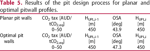
The planar and optimal pitwall profiles obtained from OptimalSlope that were employed in the pit optimization process are plotted in Figure 4. Note the profile computed by OptimalSlope exhibits a 3.4 degrees increment in OSA over the traditional one. The FoSs of all the pitwall profiles were verified by performing a LEM analysis with the rigorous Morgenstern–Price method using Rocscience Slide2 (2021). Additional stability analyses on the optimal slope profiles were also run by the finite difference method with shear strength reduction technique employing FLAC/Slope 8.1 (FLAC/Slope 2021). The critical failure mechanisms identified by Slide2 and FLAC/Slope and the associated FoS for each are reported in Figure 4(a and b). In both cases, the FoSs found are less than 1.5% from the target value of 1.30. This is a crucial verification by two independent geotechnical software that confirms the pitwall profiles found by OptimalSlope are as safe as the planar ones.
UPL pitwalls: (a) planar profile with failure mechanism (black line) and Factor of Safety determined by 2D Limit Equilibrium Method (Slide2); (b) optimal profile with failure mechanism (black line), Factor of Safety determined by 2D Limit Equilibrium Method (Slide2) and shear strain magnitude determined by Finite Difference Method with Shear Strength Reduction (FLAC/Slope); (c) Ultimate Pit Limits for different values of carbon tax for planar and optimal pitwall profiles. Images are available in colour online.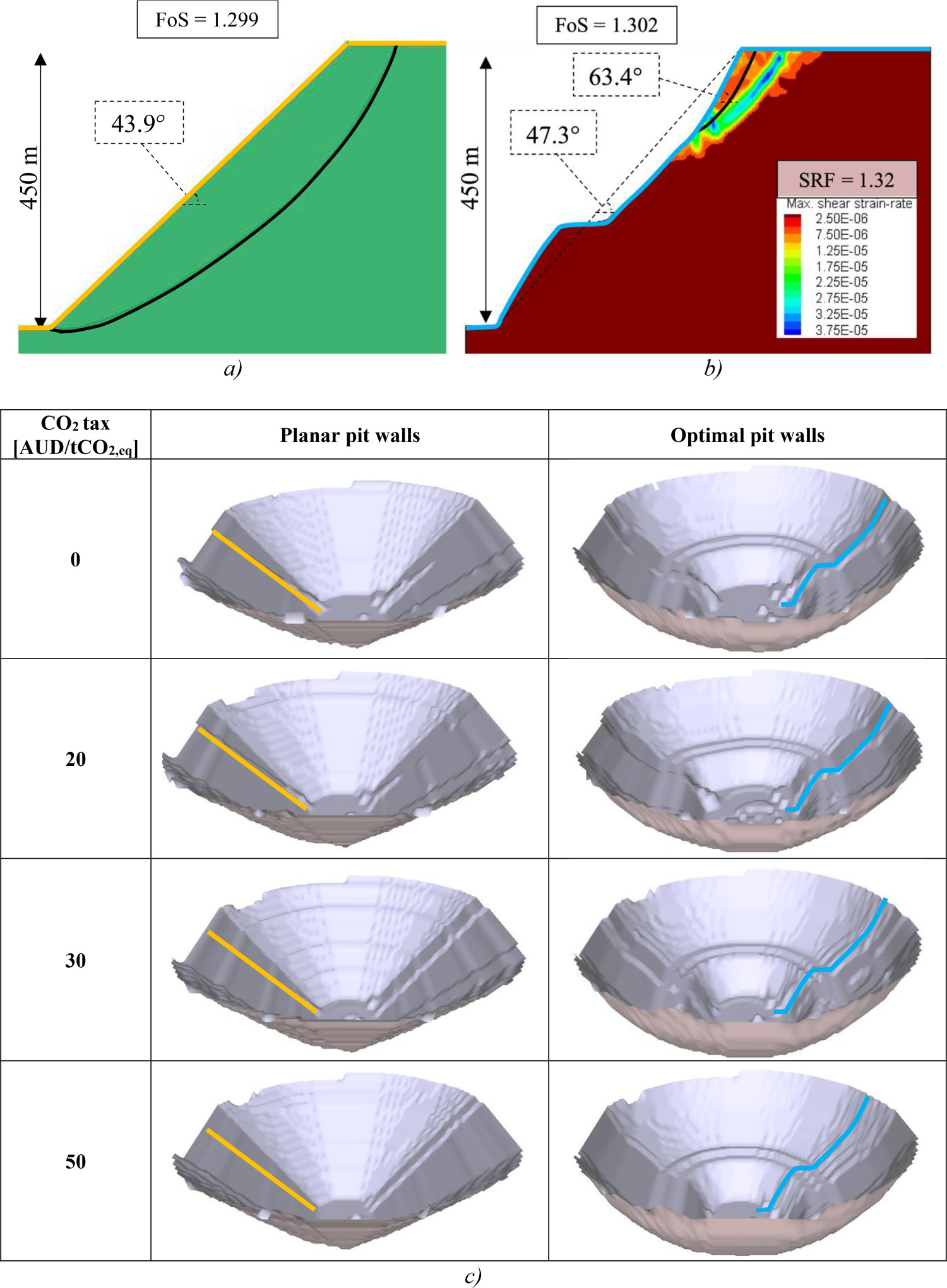
In Figure 4(c), the 3D views of the UPL computed with the pit optimization process for the designs based on planar and optimal pitwalls are plotted. As it can be expected, the size of the UPL decreases with increasing the value of the carbon tax (see Figure 4(c)).
Pit optimization results, economics, and material movement.
Pit optimization results, economics, and material movement.
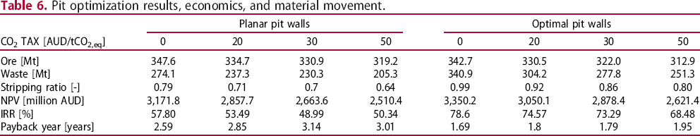
The production schedules for all the scenarios computed are plotted in Figure 5. Note that a lower quantity of rock (22 Mt/year) is extracted during the first six years, then upgraded to 40 Mt/year for the rest of the mine life. Also note that constant production over time is a highly desirable feature from a logistical point of view. From the schedule graphs, the designs with the optimal profile always extract more ore and less waste early in the life of the mine, leading to an earlier peak of the discounted cash flow curve and, therefore, a higher NPV.
Ore (orange), rock waste (grey) tonnage (vertical right axis) and discounted cash flow (left vertical axis) plotted against time in years for different values of carbon tax and slope profile shapes. Adoption of optimal profiles always allows extracting more ore and less waste early in the life of the mine. Images are available in colour online.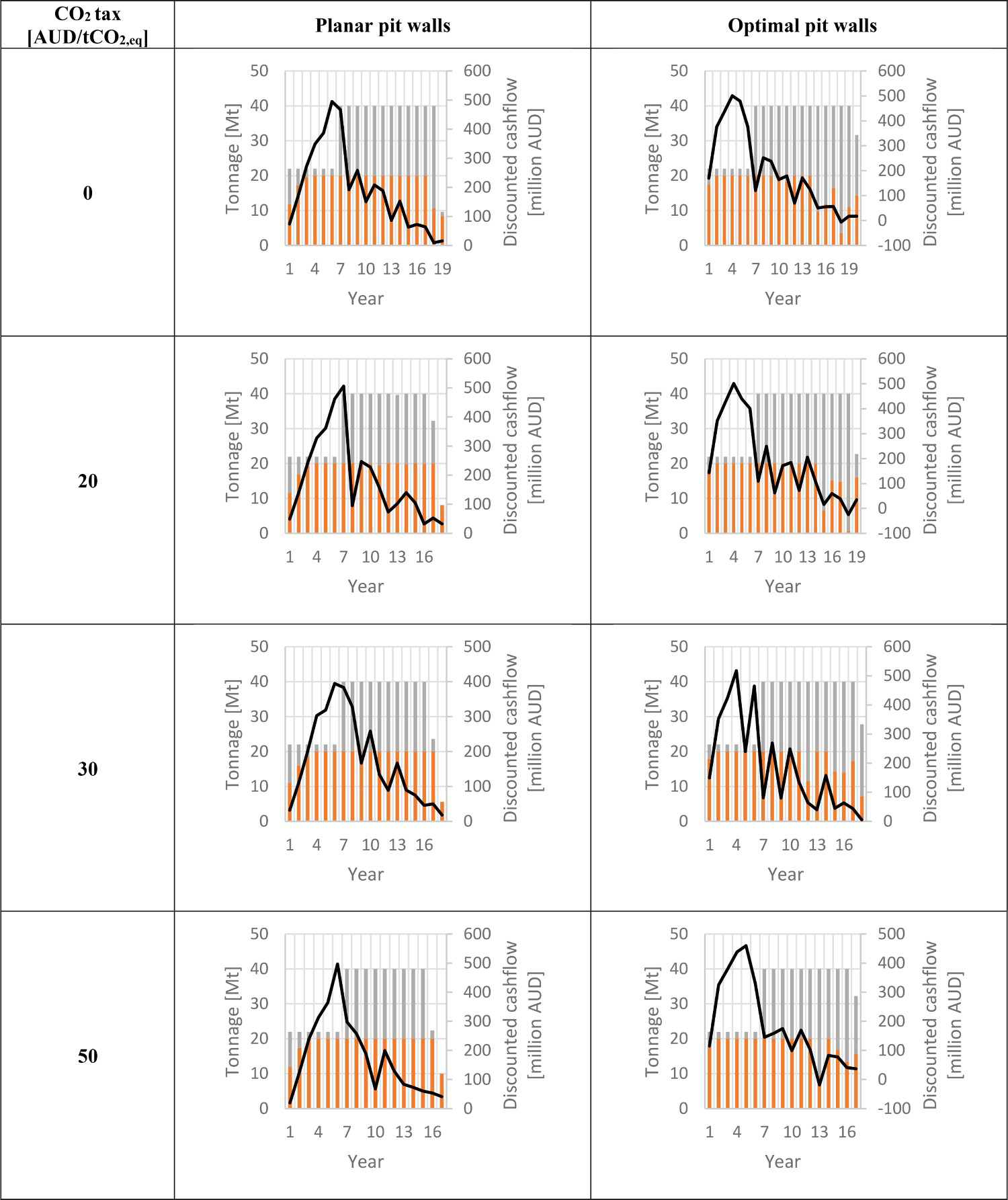
In the graph in Figure 6 the NPV against several values of carbon tax ranging from 0 AUD/tCO2,eq to 50 AUD/tCO2,eq is plotted. The datasets named ‘w/o CO2 opt’ represent cases where the pit optimization was performed without considering the carbon tax costs during the pit optimization stage. Instead, the yearly cost due to the amount of CO2 emitted was added a posteriori, by using the software ECOMINE (Zhang 2022), to the yearly cash flow and discounted to compute the total NPV. Instead, the dataset named ‘CO2 opt’ represents cases where carbon tax costs were included in the pit optimization via the methodology described in Section 3.2. From the graph emerges the points can be interpolated reasonably well by linear interpolation.
(a) Net Present Value versus carbon tax value; (b) Amount of ore extracted versus carbon tax value. The blue datasets represent the results obtained implementing the carbon tax into the pit optimization algorithm. In contrast, the red datasets showcase the cases where the carbon tax is deducted after the pit optimization stage. The datasets named ‘w/o CO2 opt’ represent cases where the pit optimization was performed without considering the carbon tax costs during the pit optimization stage. Images are available in colour online.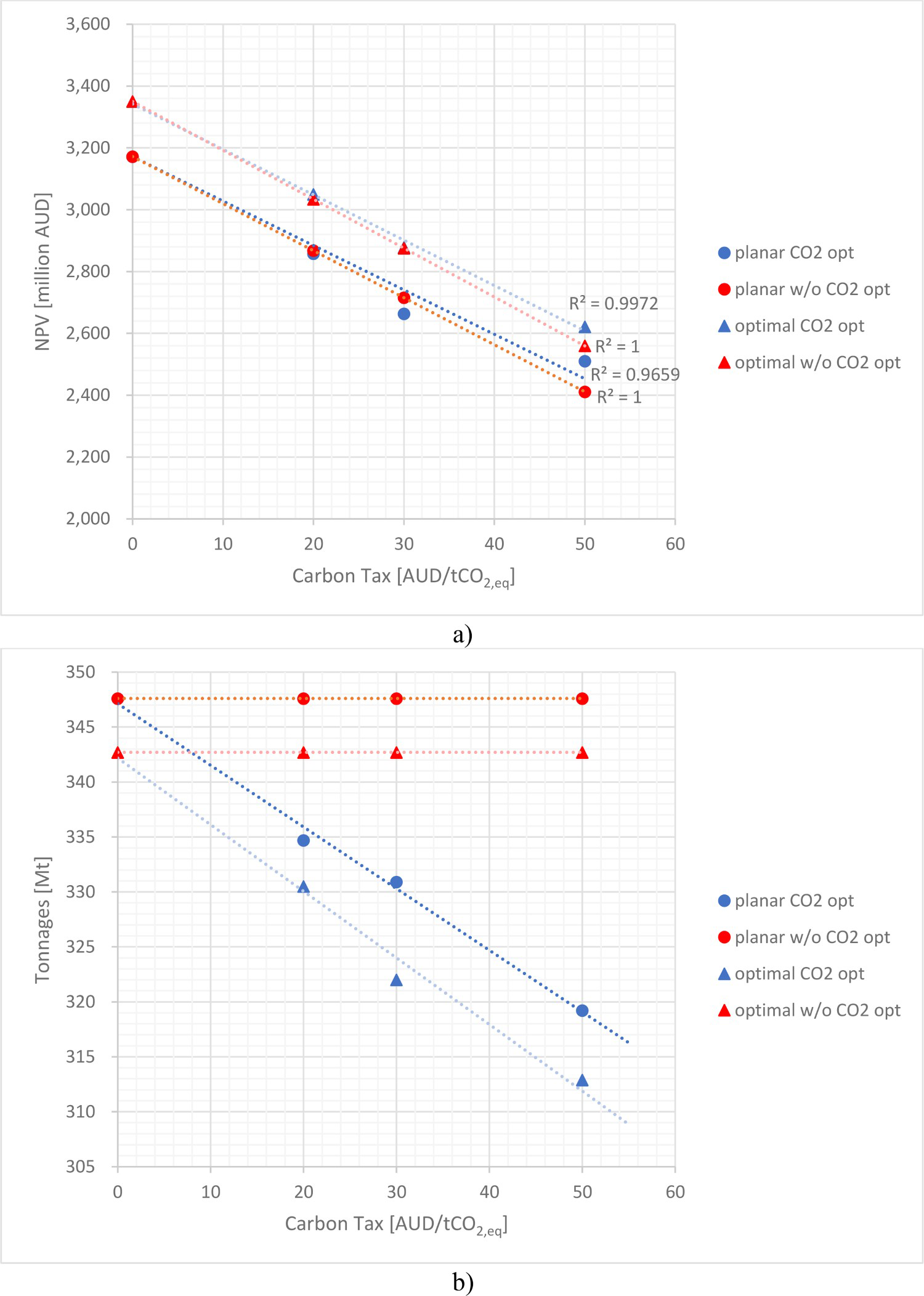
In both design methods, the linear trends suggest that considering the carbon tax costs concurrently to pit optimization (Section 3.2) leads to a significantly better NPV than not to consider them as it can be intuitively expected for any type of mining cost, i.e. adding a mining cost outside of the pit optimizer implies the pit optimization process is suboptimal. Therefore, the linear interpolations of NPV versus carbon tax show that the NPV drops less rapidly when the carbon tax is implemented into the pit optimizer than when it is not.
Another important observation is about the adoption of optimal pitwall profiles: (1) as it can be expected the NPV for the ‘CO2 opt’ case is higher than the ‘w/o CO2 opt’ one; (2) looking at the difference between the two blue lines and between the two red lines it emerges that the NPV gain due to the adoption of optimal profiles are practically constant irrespective of the value of carbon tax. This is a strong indication of the fact that the economic benefits brought by the adoption of optimal profiles can be expected to apply independently of the carbon tax scenario.
As it emerges in Section 4.2 the design based on optimal pitwalls is always financially advantageous over the design based on planar profiles so it is the obvious choice to be pursued by a mining company. In Figure 7, carbon footprint and consumed energy are plotted for all the values of carbon tax considered for the design based on optimal pitwalls. As it can be expected the amount of energy and carbon footprint reduce for increasing values of the carbon levy since the higher the levy is the higher the mining costs and therefore the cut-off grade for profitable extraction increases. It can be observed the rate of decrease for both consumed energy and emitted CO2 equivalent with the carbon tax value (Figure 7) are well interpolated linearly. This is an important finding which makes it easy in principle to extrapolate relationships that could be employed by policy makers to assess the expected consequences of setting a specific carbon tax value.
Carbon tax value versus (a) carbon footprint and (b) consumed energy for design based on optimal pitwalls. Images are available in colour online.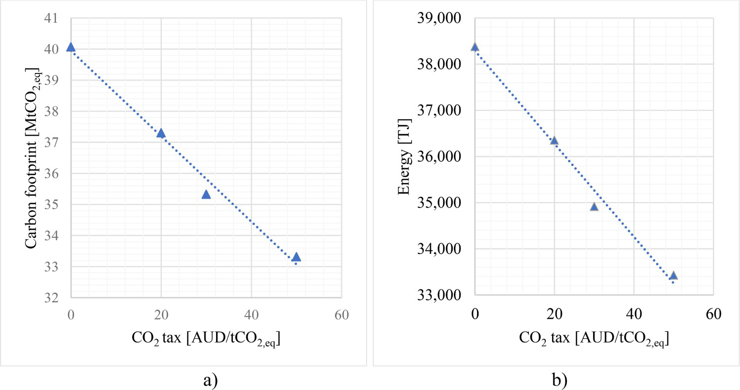
A rigorous methodology to account for the costs of a carbon levy proportional to the emissions produced by all relevant mining activities in strategic pit optimization has been introduced with the levy costs included not a posteriori but concurrently with the NPV maximization. The methodology was implemented in two commercial pit optimizers, Geovia Whittle and Datamine, which are popular with practitioners (and could be easily implemented in other commercial pit optimizers).
Several mine designs were performed for different values of carbon tax and adopting either traditional planar or non-linear optimal pitwalls for the Marvin copper deposit. The case was chosen since the mine is well known and the BM data are publicly available from the MineLib repository so the results here presented can be reproduced by anyone. In our analyses we investigated how the carbon tax value affects NPV, amount of ore extracted and carbon emissions by performing the design of the mine for four different scenarios of carbon tax values.
From the analyses, it emerges that inclusion of the carbon levy concurrently with pit optimization allows achieving substantially higher NPV than not to include it so there is a strong case for including the cost of carbon levies into the pit optimization design process. Secondly, the relationships obtained looked to be well interpolated by linear interpolation in both cases of traditional planar and optimal pitwall profiles. This is an important finding which makes it easy in principle to extrapolate relationships that could be employed by policy makers to assess the expected consequences of setting a specific carbon tax value. Of course more case studies should be considered before concluding that NPV, amount of ore extracted and carbon emissions vary linearly with the carbon tax value, but if that was to be confirmed, it points to the fact that once a sufficient number of mines have been designed accounting for the cost of a carbon levy, it would be possible for mining companies to quantitatively predict with good accuracy the effect of a prescribed carbon tax on the financial viability of a mining project and its environmental metrics. Finally, the adoption of optimal profiles realizes gains up to 215 million AUD, without compromising the safety of the UPL.
Footnotes
Acknowledgements
Author contributions:
Disclosure statement
No potential conflict of interest was reported by the author(s).
Code availability
The outputs files of OptimalSlope, Whittle, Slide2 and FLAC/Slope can be made available upon request to the corresponding author. The code to create the block model considering the CO2 tax can be downloaded from https://github.com/Agosti92/Block-model-CO2-cost-creator. The ECOMINE can be downloaded from ![]() .
.