
Abstract
This article measures and explains cost risk for IT projects compared with 22 other project types. The null hypothesis is that IT projects are not different from other projects in terms of cost risk. The thesis is falsified. IT cost risk is found to be uniquely more risky than other project types. First, we review four extant explanations of high IT cost risk: immaturity, intangibility, goal ambiguity, and stakeholder resistance. Second, we describe data to measure cost risk across 23 project types, including IT. Third, we fit theoretical distributions to the data and test for median and tail risk, showing that tail risk dominates, with IT cost risk having a fatter tail than any other project type. Fourth, we develop a taxonomy of risk based on the Pareto 1 tail parameter α, documenting that IT is uniquely risky as the only project type with α ≤ 1, indicating infinite mean and variance and, thus, infinite and unpredictable risk. Fifth, we return to the four extant explanations and conclude that, although our data do not prove the explanations, they also do not falsify them. Based on our data, we suggest two further explanations of cost risk: Bespokeness and “think-fast” decision-making, which we argue drive extreme risk and are typical of IT, with modularity and “think slow” as antidotes. Finally, we identify areas for further research.
Keywords
Introduction
How often do you restart your apps, smartphone, or laptop to fix a bug? How often do you do the same for your refrigerator or car? If you're like us, you do the former a lot more than the latter. You have a sense that IT is different: more fickle, prone to breakdown, constantly needing another update, ready to blow up in your face. In sum: more risky. 1
If you read the news, you know that your personal experience is reproduced at scale, with big government and business IT projects routinely blowing up, sometimes taking down management and whole companies with them. This happened when U.S. Health Secretary Kathleen Sebelius and TSB Bank CEO Paul Pester lost their jobs due to mismanaged IT projects (Shear, 2014; Jack, 2018) and when Kmart, a large U.S. retailer and Birmingham, the second-largest city in the United Kingdom, declared bankruptcy after failed IT system implementations (Sliwa, 2002; Clark, 2023). The prize in IT nastiness goes to the UK Post Office Horizon IT scandal, in which more than 900 postmasters were convicted of theft, fraud, and false accounting based on errors in Horizon data, with several postmasters jailed, leading to at least four suicides (Wallis, 2022). Prime Minister Rishi Sunak called the scandal one of the greatest miscarriages of justice in British history (Prime Minister’s Office, 2024). All because of unruly IT.
Explanations of IT Cost Risk
Beyond such anecdotal evidence, the research literature seems to affirm the notion that IT is particularly ungovernable and thus risky. With more than US$4.6 trillion spent on IT globally in 2024, the stakes are massive for getting governance and risk right (Gartner, 2023). Even small errors will matter. Decades ago, Brooks (1987, p. 10) lamented that IT projects are “capable of becoming a monster of missed schedules, blown budgets, and flawed products.” Such “monster” projects “differ profoundly,” Brooks argued, from other things humans build, e.g., houses or automobiles (p. 11). Unfortunately, Brooks never presented systematic data to support his claim of the profound difference between IT and other projects, and—also, unfortunately—neither has anyone else. Nevertheless, the extant literature, which we review here, identifies four attributes of IT projects—immaturity, intangibility, goal ambiguity, and stakeholder resistance—that supposedly make IT more risky than other project types, including for cost risk—or “blown budgets,” in Brooks’s words—which is our focus here. 2
First, it is argued that IT is more immature than other project types. As a discipline, IT is younger than most, with its age measured in decades. In contrast, construction engineering dates back centuries, if not millennia, which means it has had time to build and refine experience, standards, processes, building codes, legislation, and so forth. Nothing similar exists in IT, which, in this sense, is significantly less mature than other engineering and technology disciplines, including for costing (Shaw, 1990). In fact, the term “IT” only began to appear around 1990 in documents from the International Organization for Standardization (ISO) (Ralston et al., 2003). Moreover, unlike other engineering disciplines, IT is not regulated and one cannot obtain professional licensure. IT is also young as an academic field, resulting in relatively weak theory and data compared with other disciplines. This means that the field is less professionalized, again indicating its relative immaturity in comparison with other engineering disciplines. Finally, IT is typically also not regulated by public safety or planning commissions, unlike more tangible project types, such as buildings, power plants, roads, dams, mines, and so forth, which are subject to extensive oversight by regulators. Instead, IT projects are generally governed by internal management that oversees their progress, resulting in higher risk for IT projects, or so the immaturity argument claims.
Second, it is also argued that the core of most IT projects—software—is more intangible than other project types. That is, IT is not embedded in Euclidian space as we know it, like other projects are. Behavioral science has long documented that the human brain is generally unsuited for grasping non-Euclidian geometry, including nonlinear relationships. For software, Brooks (1987, p. 12) rightly observed that IT “has no ready geometric representation in the way that land has maps, silicon chips have diagrams, computers have connectivity schematics.” The intangibility of software also means that there are no physically tangible milestones against which to measure progress as there are for a physical product. This makes it difficult to visualize and detect problems compared to, for example, a physical building. It also makes it more difficult for clients and vendors to understand each other and develop a common view of what it is they are building. Visible signs of programming progress are often lacking or, if they exist, are ambiguous. Due to such intangibility, progress and status reporting often suffer from error and optimism bias (Brooks, 1975; Flyvbjerg & Budzier, 2011; Snow et al., 2007). To complicate matters further, IT projects depend on the joint optimization of software components and social components, for instance, in change management projects (Avgerou et al., 2007; Dobson & Nicholson, 2018; Lyytinen & Newman, 2008; Markus & Robey, 1988; Sarker et al., 2019). According to the literature, the intangible nature of IT projects tends to make them more risky than other projects, with poorer performance, including for cost. 3
Intangibility entails malleability, which leads to further risk. Schmidt et al. (2001) identified changing scope and requirements volatility as being among the top 10 risk factors that affect IT projects. Change requests to enhance or alter software functionality are routine, directly from senior management or users, indirectly from changes in the underlying systems, and the need to interface with other information systems. To be sure, changing scope and requirements apply to other project types as well, for example buildings. But, because the intangibility of software makes it more malleable than other project types, it is easier and less costly (at least initially) to alter software, which offers opportunities for continuous change (Yoo et al., 2010). Brooks (1987, p. 12) rightly observed: “Buildings do, in fact, get changed, but the high costs of change, understood by all, serve to dampen the whims of the changers.” For software, because of its intangibility and malleability, there are fewer restrictions on the “whims” of clients, users, and developers who are, therefore, less likely to restrain themselves from making change requests. In this manner, the social components of IT projects further contribute to their malleability (Nielsen et al., 2014). As a result, IT projects appear to be particularly prone to scope creep, which is a classic driver of project cost and schedule risk. A final aspect of malleability and risk is that IT is typically not built from a blank slate. Projects are implemented in a running concern with poorly documented IT infrastructure. They must be patched into and onto extant systems with extensive modifications, tweaks, data migrations, and workarounds to effectively integrate with legacy systems, adding to malleability and interdependencies. Integration not only increases costs directly related to the additional work required but also increases the transaction cost for transferring knowledge about the idiosyncrasies of the business and its IT to contractors involved in projects (Dibbern et al., 2008; Larsen et al., 2013). Integration with added interdependence creates challenges, according to project management scholars (Gregory et al., 2015; Perrow, 1999). Drawing on the concept of self-organized criticality, Flyvbjerg et al. (2022) illustrated that interdependencies among technological components in an IT system can be a source of extreme cost risk. In essence, changes or problems in one technological component can have cascading effects on other interdependent technological components. Consequently, one component can affect many others, leading to the kind of nonlinear effects that Brooks alluded to above. The cost and duration of this type of interdependent integration are difficult to estimate ex ante, further adding to project risk. The situation for IT is a bit like surgery on the human body—you often do not know what you will find before you get in there and start cutting around.
Third, scholars have observed a high degree of goal ambiguity in IT projects. This could possibly be considered a further aspect of intangibility. Typically, however, it is singled out as an attribute of its own. According to goal-setting theory, unambiguous goals reduce the variability of performance, whereas ambiguous goals lead to greater variation (Locke et al., 1989). The absence of clear goals leads to requirements volatility and scope creep, and thus higher cost risk. Software projects are considered nonphysical “soft projects,” as mentioned above. It’s called software for a reason. Crawford and Pollack (2004, p. 646) suggest that “the goals and objectives of soft projects are typically not clearly defined at the outset.” Again, IT projects are not the only project type with goal ambiguity. It is argued, however, that plausibly, IT projects tend to have greater goal ambiguity relative to “hard projects,” in which goals are more readily defined. Moreover, the extant literature suggests that goal ambiguity can impede cooperation in integration teams working on enterprise system programs (Chang et al., 2019). Based on a case study involving IT project escalation, Mähring and Keil (2008, p. 255) further reported that the first phase of the escalation process is marked by “drift, in which the project is allowed to continue and consume resources as ambiguity concerning the project charter and conflicts concerning project goal and direction emerge.” In a subsequent experiment, Lee et al. (2012) found that an ambiguous budget and schedule goal was more likely to cause software project escalation to occur as compared with a clear and specific goal. Project escalation directly drives cost and schedule risk. Finally, malleability, as identified above, further adds to goal ambiguity, resulting in the type of amplification between variables that has been documented to generate extreme risk (Taleb, 2020).
Fourth, scholars have long observed that IT projects are often difficult to implement due to stakeholder resistance, internal and external (Hirchheim & Newman, 1988; Keen, 1981; Markus, 1983). For external resistance, IT has been argued to be particularly permeable to outside stakeholders, in the sense defined by Crawford and Pollack (2004, p. 648), that is, as the degree to which a project’s “goals, processes and outcomes are affected by influences outside project control.” A project that can be isolated from its environment is more readily controlled than one that cannot. While IT projects are not the only type of project that exhibits project permeability, it is plausible that such projects tend to have greater permeability relative to projects that are less subject to external and stakeholder influences. IT projects are said to have a high degree of permeability because they impact many parts of the organization undertaking the project and thus have numerous stakeholders outside the project whose needs must be satisfied. Also, because IT projects are “soft projects,” it is more difficult to get these stakeholders to agree on concrete goals and system requirements and keep their interests aligned throughout the project. Moreover, IT projects typically involve developing software that must integrate with other systems, either inside or outside the organization. Finally, IT projects often involve contractors or outsourcing companies that are integral to the project’s success but external to the organization and thus represent permeability and associated control challenges (Gregory et al., 2013).
For internal resistance, IT projects are said to be more prone to such resistance—that is, resistance from within the organization doing the project—than other project types. Target users of the IT in question are seen as particularly strong sources of resistance. This is because many IT projects are change projects that fundamentally alter internal workflows and power dynamics within an organization (Joshi, 1991; Kim & Kankanhalli, 2009; Lapointe & Rivard, 2005; Marakas & Hornik, 1996; Martinko et al., 1996). According to behavioral science, humans are generally hardwired with a “conservatism bias,” which makes us resist such change (Edwards, 1968). In a classic study, Markus (1983) concluded that when people believe that a system may cause them to lose power, they will resist it. As always in human affairs, power is a key explanatory variable, and while stakeholder resistance is not unique to IT projects, the literature suggests it is likely to be stronger here than for other project types. This is because, more than other project types, IT projects are change projects designed to alter organizational processes and workflows with consequences for organizational power. As such, IT projects tend to create pockets of resistance among key internal stakeholders whose routines are disrupted and whose power, including job security, may be threatened. In consequence, the implementations of IT projects are often fraught with obstacles that may not affect other project types to the same degree. Again, this would tend to drive IT cost risk to higher levels than for other project types.
In sum, according to the extant literature, each of the four attributes identified above—immaturity, intangibility, goal ambiguity, and stakeholder resistance—is likely to amplify IT cost risk. Other project types undoubtedly share some of the attributes. It is argued, however, that (1) each of the attributes tends to be stronger for IT and (2) IT projects are particularly prone to being subject to all four attributes at once, both of which would be mechanisms for driving cost risk to a higher level for IT than for other project types, as the literature argues is the case. Each attribute may be considered a variable that causes cost risk. Taken together, the four variables may be considered a theory that explains IT cost risk and why such risk is higher than for other project types. The theory is illustrated by the causal diagram in Figure 1. Expressed in conventional mathematical terms, the theory accounts for P(A/E∣I1, I2, G, S), where P is the observed frequency of A/E (risk), A is the actual cost of the project, E is the estimated cost, with the frequency conditional on the degree of immaturity (I1), intangibility (I2), goal ambiguity (G), and stakeholder resistance (S). We see that multiple factors impact the outcome and that none of them is deterministic. The factors determine, however, the probability of outcomes and, thus, the distribution of cost risk.
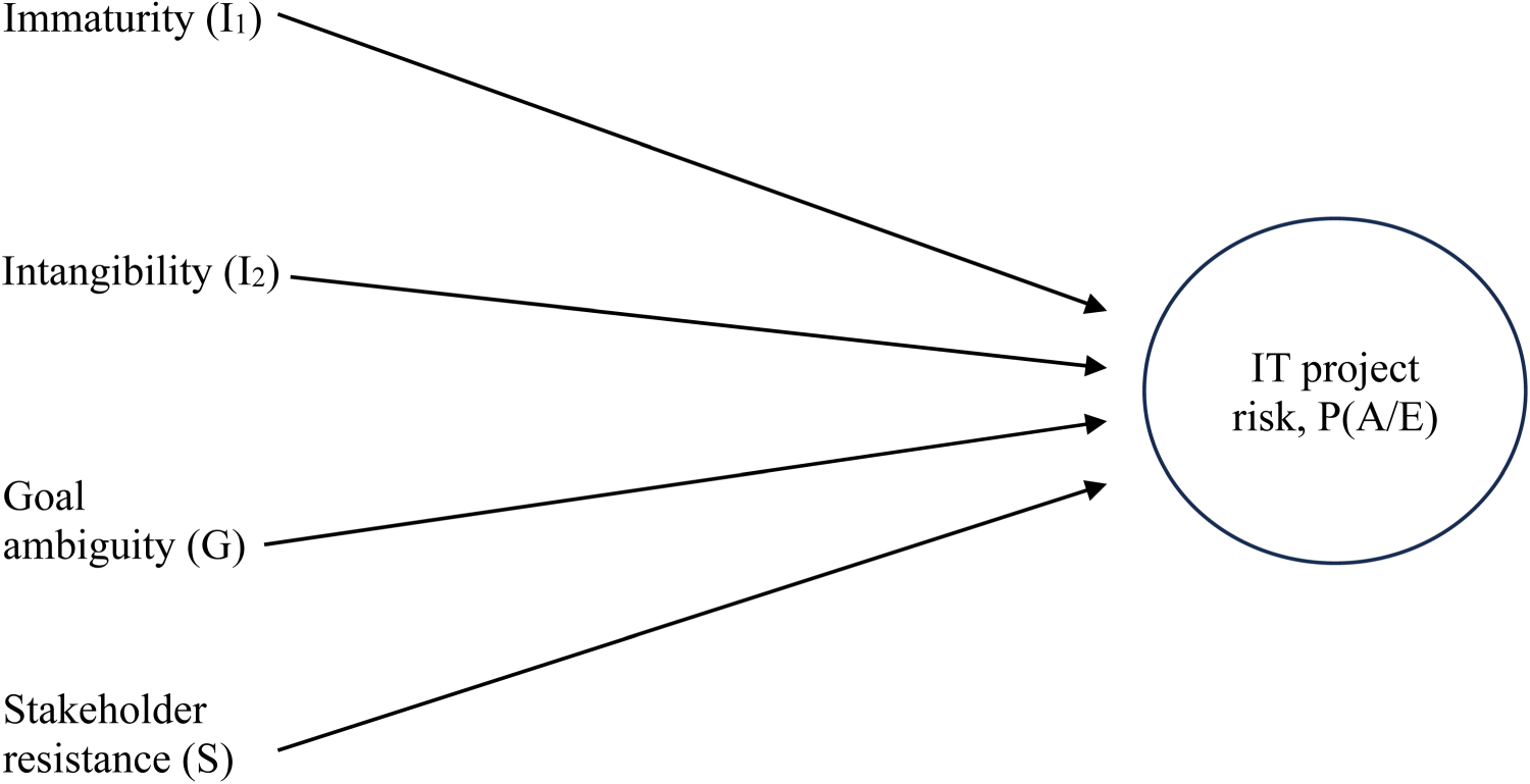
Causes of IT project risk, including cost risk.
There is a problem with the theory, however. It has never been systematically tested, even if the extant literature often reads as if it has, c.f., Brooks above. As explained in Flyvbjerg et al. (2022, pp. 610–612), the sample sizes used thus far in scholarship on IT cost risk are far too small to produce valid and reliable findings.
4
Small samples suffer from statistical noise and are typically not representative of the population. As a consequence, the literature, the four attributes, and the theory must, for now, be considered plausible but unsubstantiated guesses. For substantiation, at a minimum, it must be documented for a large representative sample that IT cost risk is indeed larger than for other project types, that is, P(extreme A/E)IT > P(extreme A/E)other. If this proves not to be the case, the theory and its explanations in terms of the four attributes would have been falsified. Based on a large sample of IT projects, Flyvbjerg et al. (2022) systematically documented that IT projects are indeed extremely risky. But no cross-group comparisons were made with other project types, and none exists in the literature (see Appendix A). Below we carry out such a comparison across 23 project types, testing the following null hypothesis: H0: IT cost risk is no different from the cost risk of other project types.
Or expressed mathematically:

Data and Methods
In Flyvbjerg et al. (2022) we did a within-group analysis of IT project cost risk, documenting infinite, unpredictable cost risk for IT projects. Here, we add 22 project types other than IT and conduct a cross-group analysis to test whether IT cost risk is similar to cost risk for other project types. We collected data on three main types of project risk: cost risk, schedule risk, and benefit risk. Here we focus on cost risk. The dataset is a much-expanded version of data previously analyzed, in, for example, Flyvbjerg et al. (2021, 2022) and Flyvbjerg and Bester (2021). The data have never been used before for a cross-group comparison of IT with other project types. Cost risk and cost data are considered particularly important objects of study, because delivering projects within budget is a key dimension of project performance (Baccarini, 1999; Kirsch & Beath, 1996; Nidumolu, 1995). Moreover, cost overruns can undermine an organization’s profitability, its reputation, and, for big projects, even its survival.
In total, we collected cost data on 11,011 projects across the 23 project types listed and defined in Appendix C. Geographically, the projects are located in 126 countries on six continents; historically, the majority of projects have been completed recently, in the 21st century. The average project size ranges from US$29 million to US$16 billion in 2020 prices. Average project duration varies from one to 14 years, measured from the final investment decision to going live. The data cover both government and business projects. The total value of the project portfolio is US$4.64 trillion in 2023 prices. The sample is 45 times larger than the average sample size of the identified studies comparing performance across project types and 15 times larger than the biggest previous sample (see Appendix A).
We follow standard practice going back to Pickrell (1990) and measure cost risk by cost overrun, defined as actual divided by estimated cost in real terms, baselined in the estimate at the time of the final investment decision (FID). 5 A value of one represents on-budget delivery, above one over budget, and below one under budget. For example, a value of 1.40 would show an overrun of 40% for that project type, on average, measured from the FID until going live. To measure cost overrun on individual projects, we collected data on estimated and actual cost. The data were collected from two main sources: (1) directly from owners of projects, based on their accounts; and (2) from public sources, for example, auditor reports, official reports, and academic research. Only high-quality data, that is, data based on valid and reliable written records, were included, which means we did not collect data from less reliable sources—such as interviews, questionnaires, newspaper articles, and non-peer-reviewed conference papers—to avoid the biases and errors associated with these sources. For analysis, we included project types for which we had data for 10 or more projects. Appendix B provides additional information on data collection.
For conventional descriptive analysis of average and median risk, we studied all 11,011 projects and all 23 project types. For the analysis of tail risk, which turned out to be the more important type of risk, we focused on the upper tail, that is, projects with an overrun above 1, amounting to 5,596 projects, again for all 23 project types. We built on Clauset et al. (2009) to fit a Pareto 1 distribution to the data. We added visual inspection using QQ plots of probability distributions for each project type. We supplemented this with Pareto and lognormal goodness-of-fit tests using the Anderson-Darling test, the Chi-square test, and the Approximate Kolmogorov-Smirnov test. Finally, we did a nonparametric bootstrap analysis of α values before settling on the Pareto 1. Appendix D provides a detailed explanation of the statistical analyses employed, including robustness tests.
Extensive robustness tests were considered particularly important to ensure our findings were not artifacts of how we collected, classified, or analyzed the data. First, we ensured that only high-quality data were included in the study, as mentioned. Second, we made sure to collect data from different types of sources and tested whether our findings were robust across sources, which was the case. This test was particularly important because differences in variance between different data sources may spuriously generate fat tails, which would then be an artifact of data collection, not a characteristic of the data. We established that the fat tails were not artificial in this manner. Third, we tested for robustness of results across project size, project duration, and year of going live, again to ensure the fat tails identified were not generated as artifacts of mixing data that should not have been mixed, that is, data from different project populations. Fourth, we tested different ways of categorizing the data according to project type and found that our findings were robust across different taxonomies. Finally, whenever different statistical methods existed for testing our hypotheses, we used all of them to test whether our results were robust across methods, which was the case. In sum, the robustness tests documented that the results presented below are real traits of the data and not of how the data were collected, categorized, or analyzed. The robustness tests are further described in Appendices B and D.
Finally, the data may have a conservative selection bias—that is, projects in the project population may perform worse than projects in the sample. This is because, as mentioned, we collected data only on projects for which high-quality written records were available. However, organizations that keep high-quality records and are willing to share those for research purposes are generally considered more mature in their project management practices than average organizations, producing better outcomes (Flyvbjerg et al., 2022). This bias should be kept in mind when interpreting the findings in the Results section below.
Results
After having accounted above for the extant literature, our data, and our methods, in this section we present our results by:
Presenting descriptive statistics on cost overrun for each of the 23 project types; Testing which probability distributions best fit the observed data for each project type; Comparing IT cost risk with cost risk for 22 other project types; and Systematically classifying cost risk based on the tail parameter α, finding that IT tail risk is in a class of its own as the only project type with α ≤ 1, showing infinite, unpredictable cost risk for IT, more extreme than for any other project type.
In presenting the results, we focus on cost risk. It should be noted, however, that in preliminary analyses of schedule risk, we found similar results as for cost risk, although with weaker support because of smaller sample sizes. Analyses of benefit risk could not be conducted due to lack of data.
Descriptive Statistics for Cost Overrun
Table 1 shows the mean and median cost overrun for each project type. We see that IT stands out with a large difference between the mean and median of 73 percentage points. A large difference is a known indicator of possible fat tails. 6 Indeed, Flyvbjerg et al. (2022) documented that IT cost overrun follows a power-law distribution with an extremely fat tail.
Cost Overrun per Project Type, Ranked by Mean, N = 11,011
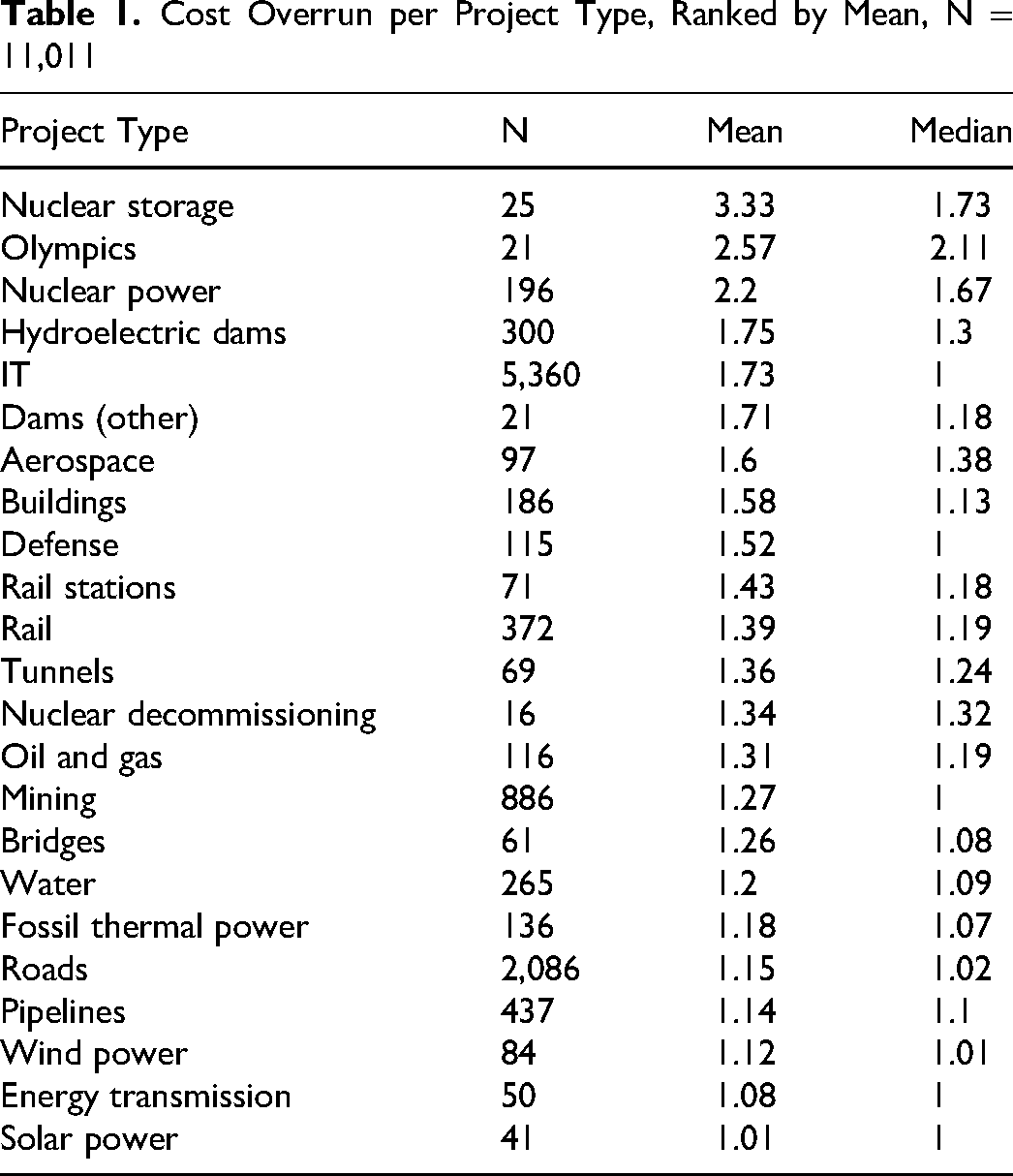
A closer look at Table 1 indicates that some project types appear to have similar means and medians. The three project types with the lowest mean (solar power, energy transmission, wind power) also have low medians. Moreover, the mean and median are close, indicating a more symmetric distribution than observed for IT and other project types. Similarly, the three project types with the highest mean (nuclear storage, Olympics, nuclear power) also have some of the highest medians. IT distinguishes itself by having a low median of 1 (lower than most project types) while having a high mean of 1.73 (higher than most).
Table 2 shows, for each project type, the percentage of projects with extreme overrun (here defined as the part of the upper tail with an overrun larger than 50%). Again, we see that IT stands out, with the largest mean value of extreme overruns at 5.53, that is, a mean overrun in the tail of 453%. This is the average in the tail, meaning that many IT projects have an even larger overrun. Only nuclear waste storage comes close to IT, with an average overrun in the tail of 5.27. In terms of cost risk, Table 2 shows that if you are planning an IT project, your base rates are an 18.26% risk of ending up in the tail with an expected overrun of 453% and a substantial risk of further overrun above this.
Frequency of Cost Overruns per Project Type, Ranked by Mean in Tail, N = 11,011
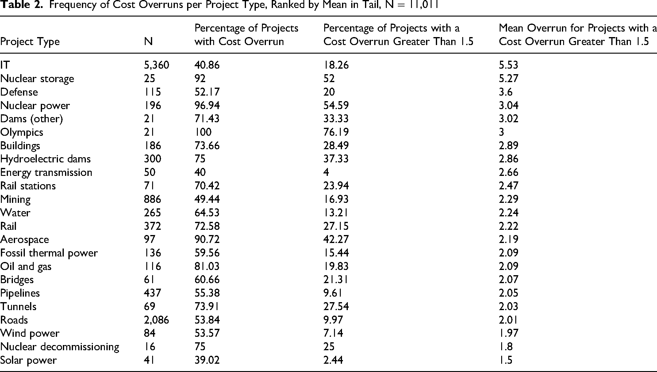
Table 2 further shows that cost overruns are more frequent than not in 19 out of the 23 project types. Notably, IT has one of the lowest frequencies of cost overruns (40.86%)—along with energy transmission (40.00%) and solar power (39.02%). On the opposite end of the scale, we find aerospace (90.72%), nuclear storage (92%), nuclear power (96.94%), and the Olympics (100%), where projects go over budget with near certainty.
In sum, Table 2 illustrates an interesting dual character of IT cost risk. On the one hand, more IT projects are actually delivered on budget than for most other project types. On the other hand, a substantial fraction of IT projects has larger cost overruns than other projects. This distribution has informally been called “barbell” shaped and is well-known in financial markets, lending its name to the so-called “barbell strategy” for mitigating risk, described by Taleb (2010, 2020). Worth noting here is that the “barbell” is an indicator of possible extreme cost risk. Following, we test whether such risk is unique to IT by fitting probability distributions to cost overruns for 23 different project types, including IT.
Fitting Probability Distributions
As mentioned above, Flyvbjerg et al. (2022) previously documented that IT cost overrun is fat-tailed. Here, we test whether IT cost overrun is more fat-tailed—and thereby riskier—than other project types. This has never been done before.
For fat-tailed distributions, customary statistics like the mean and standard deviation do not sufficiently capture the relevant information about the distribution. The information is in the tail, often to a degree where just a few extreme values determine the size of the moments of the distribution (mean, variance, skew, kurtosis) and possibly whether the moments are finite. 7 We, therefore, need to measure the fatness of the tail directly to understand real variance and, thus, real risk. We do this by fitting theoretical distributions to the tail for each project type and calculating the shape parameter for the tail. We then compare IT with the other project types based on the size of the tail parameter.
As in Flyvbjerg et al. (2022), we built on the procedure suggested by Clauset et al. (2009) and conducted goodness-of-fit tests (Anderson-Darling, Chi-square, Kolmogorov-Smirnov) against many candidate probability distributions (e.g., normal, lognormal, Weibull, beta, and Pareto) fitted to the observed data in the upper tail (see Appendix D for details).
The results suggest that for most project types, the Pareto 1 distribution
8
provides the best fit to the data.
9
The Pareto 1 is a power-law distribution with the cumulative distribution function (CDF) defined as: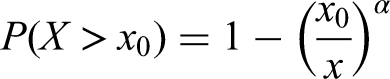
If we plot the function in a log-log diagram, it is a straight line falling from left to right, with minus α measuring the slope of the line. Table 3 summarizes the relationship between α and the statistical moments: mean, variance, skew, and kurtosis.
Statistical Consequences of Fat Tails
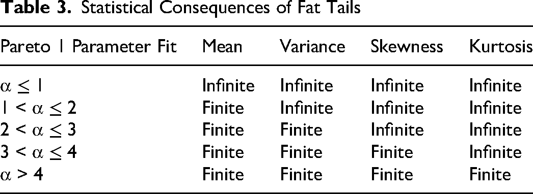
Based on the properties of the Pareto 1 distribution, we describe the consequences associated with the various ranges of values that α can have:
α ≤ 1: Infinite mean, designating infinite risk. Conventional statistics that assume the existence of the mean are useless, and conventional prediction, by which we understand forecasting based on the mean, is impossible.
10
The law of large numbers is too slow to converge for the mean. This is the most extreme risk that exists, according to the Pareto 1, called “wild” risk by Mandelbrot (1997); 1 < α ≤ 2: Infinite variance, that is, infinite and unpredictable risk. The law of large numbers will converge to the mean, in theory, but often too slowly for practical purposes; 2 < α ≤ 3: Mean and variance are both finite. Skew and kurtosis, however, are infinite, meaning that conventional statistics based on these will fail. Skew is a measure of the asymmetry of a distribution about its mean. Infinite skew means that one side of the distribution dominates the other. For cost overruns, which we study here, this would mean that a portfolio of investments would not balance out. For large samples, although the law of large numbers begins to converge for the mean, this is again often too slowly for practical purposes; 3 < α ≤ 4: Kurtosis is infinite, so statistics that require a finite value for it will fail. Kurtosis is a measure of the relative importance of the tails of a probability distribution as compared to its center and shoulders. Infinite kurtosis means that observations in the tail, for example, extreme cost overruns, dominate the distribution. The law of large numbers converges less slowly; and α > 4: Mean, variance, skew, and kurtosis are all finite, that is, statistics that depend on them are valid; the law of large numbers converges quickly. Risk is “mild,” in Mandelbrot’s terms.
In sum, for α above 4, tails are thin, and regression to the mean applies together with conventional statistics. For α below or equal to 2, tails are extremely fat, resulting in regression to the tail, where conventional statistics that assume a finite value of mean and variance do not apply, just as the law of large numbers does not or is too slow to converge for the mean (Flyvbjerg et al., 2020). Here, it is interesting to note that when the true α (α in the population) is less than 2.5, we would need a sample of more than 1,000 observations to prove that it is significantly different from 2 (the threshold for infinite variance). Flyvbjerg et al. (2022, pp. 610–612) show that the average sample size for studies that measured IT project performance, including cost overrun, is 74 projects (max. 170), that is, more than 10 times smaller than the 1,000 projects needed to estimate α with acceptable certainty. When α is smaller than 2.5—and α is significantly smaller than this for IT, as we will see—the sample size would have to be significantly larger. We therefore conclude that the sample sizes used in previous studies are too small to reliably estimate α and, thus, IT cost risk.
For α between 2 and 4, the situation falls between regression to the mean and regression to the tail, with the law of large numbers converging for mean and variance in principle. But for practical purposes, the law will often be too slow in the sense that samples would have to be prohibitively large for estimates to converge, which is to say that the time and funds to establish such samples would typically not be available in practice. In forecasting, when higher moments are infinite, decision-makers face unbounded uncertainty for both individual project decisions and portfolios of decisions.
Comparing IT with Other Project Types
Figure 2 shows the α values for each project type (black vertical lines) with 95% bootstrapped confidence intervals (gray horizontal lines). Again, IT stands out with the lowest α value of any project type. Moreover, the α value for IT (0.92) is less than one, which is a crucial finding in terms of risk because α values less than or equal to 1 indicate the most extreme and unpredictable type of risk that exists, as explained above. IT is alone among the 23 project types studied in being exposed to this special category of extreme risk. Only one other project type comes close to the unpredictability and risks associated with IT projects, namely nuclear storage, with an α value of 1.05. This surprising result means that, at the time of the final investment decision, the actual cost of an IT project is more unpredictable and involves more extreme risk than for any other project type, including the disposal and storage of nuclear waste. This is all the more astonishing, given the fact that IT projects have a much shorter duration on average than other project types, and shorter duration supposedly means lower risk, other things being equal (see further in the Discussion section). Most people would probably consider the management of nuclear storage significantly more risky than the management of IT, including in terms of cost risk. So why is this not the case? We return to this question in the Discussion section.
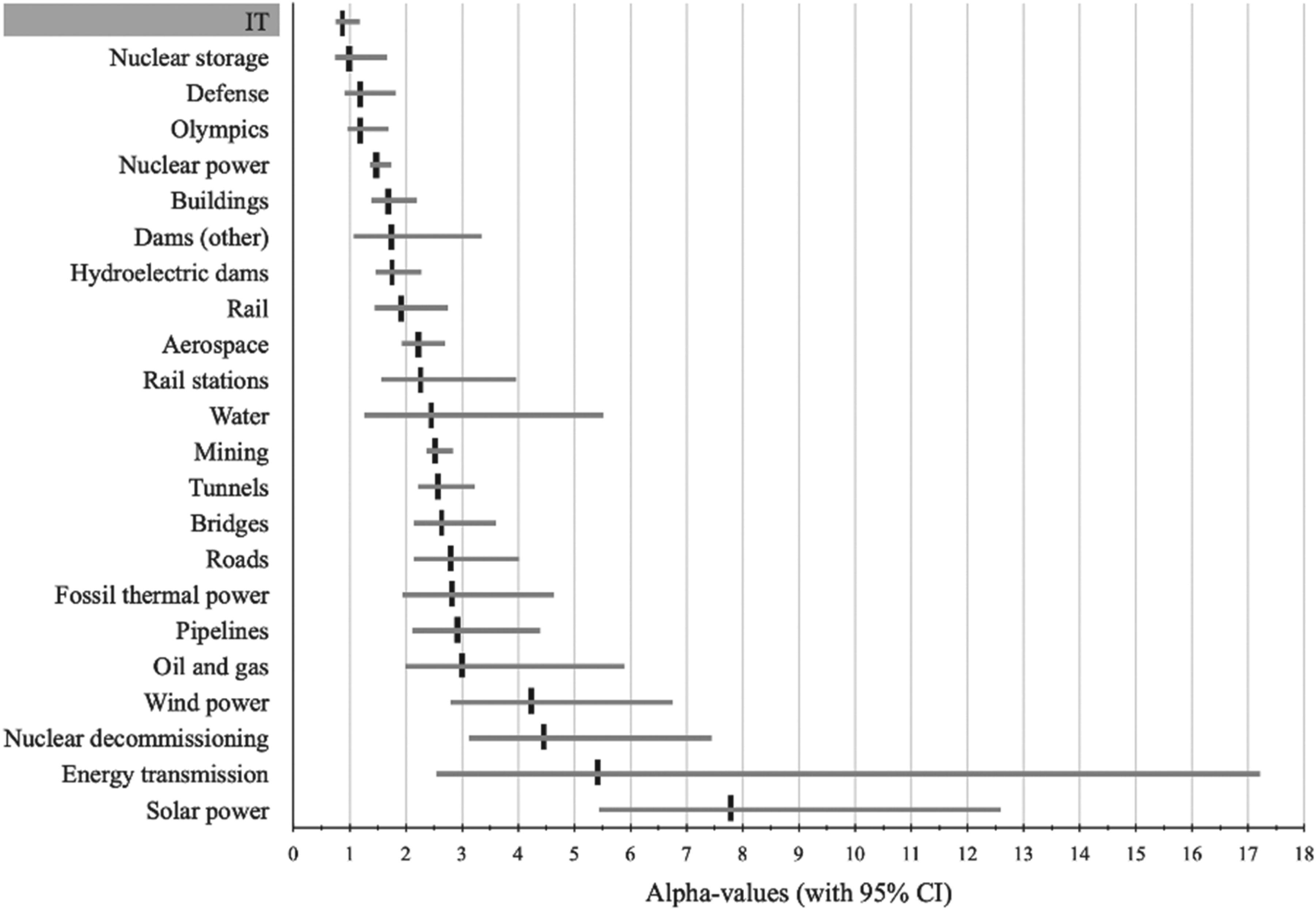
Bootstrapped median alpha values for upper tail, per project type, with 95% confidence interval (CI), N = 11,011.
As depicted in Figure 2, defense and the Olympics also have low α values, with their 95% confidence intervals including α values of 1 or below, indicating the possibility of the most extreme form of cost risk for these project types as well. At the opposite end of the scale, we find solar power with an α value far greater than 4 (including the values covered by the confidence interval), indicating that extreme cost overruns are much less common. 11
Figure 3 visually illustrates the fatness of tails by depicting the cumulative distribution function for the five project types (IT, roads, mining, rail, and pipelines) with the largest number of projects in the upper tail. 12 The horizontal axis shows cost overrun, whereas the vertical axis shows the complementary cumulative probability (i.e., the probability of observing a cost overrun greater than or equal to a specific level on the horizontal axis). The curve shows how the probability of encountering a cost overrun above a certain size decreases as the size of the overrun increases. Alpha is a measure of the steepness of the curve. The lower the α, the flatter the curve and the fatter the tail. The fatter the tail, the higher the likelihood of extreme cost overrun.
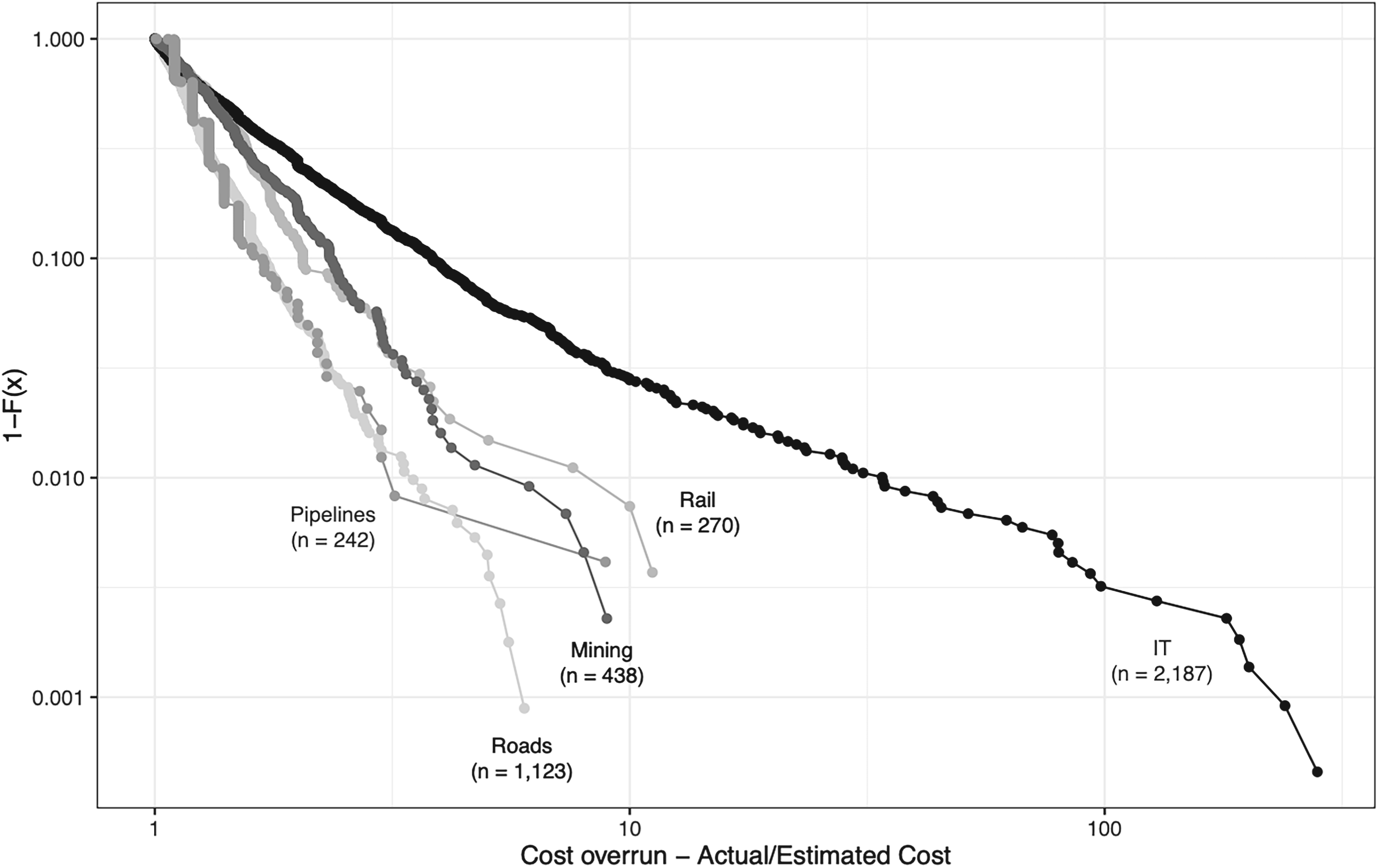
Complementary cumulative distribution functions (CDF) for the five project types with largest samples in the tail.
Here, too, IT stands out, having by far the longest and fattest tail for cost risk. Clearly, someone doing an IT project is facing a very different risk profile than someone doing a road or rail project. Again, this is surprising given the fact that road and rail projects take much longer to complete than IT projects. IT is extremely more risky than other project types, something for IT owners, planners, and managers to keep in mind and mitigate.
A Taxonomy of Risk
Empirically, our main finding is that IT cost risk, measured by cost overrun, is in a category of its own, being uniquely extreme and uniquely unpredictable. Table 4 summarizes this finding by classifying each of the 23 project types into one of five distinct risk categories based on α values and their statistical consequences for risk prediction and risk management, as depicted in Table 3.
Cost Risk Categories Based on Alpha Values (see also Table 3)
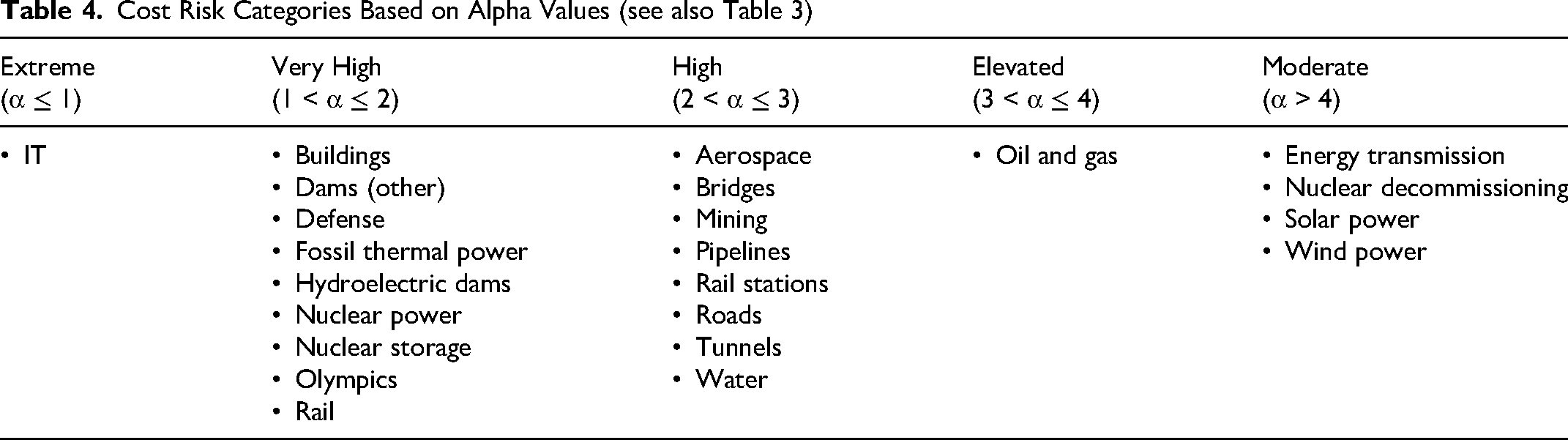
For the category of extreme risk, the mean is infinite. For projects in this category (here, only IT), the risk may be mitigated, but it cannot be predicted by conventional methods. The law of regression to the tail applies (Flyvbjerg, 2020). Conventional assumptions of normal or near-normal distributions, which are common in IT risk management and forecasting, do not apply. 13 They will grossly underestimate tail risk (Flyvbjerg et al., 2022). Ignoring fat-tailed, high-impact risk exposes organizations to suboptimal decision-making with potentially devastating financial consequences. This is, today, the situation for IT decision-making.
For the category of very high risk, variance is infinite, whereas the mean is finite, that is, the mean exists. Infinite variance means that the law of regression to the tail applies whereas, again, the law of regression to the mean does not. 14 For projects in this category, such as buildings and nuclear power, the risk is somewhat less explosive than for IT, but it is still very fat tailed and unpredictable with a high risk of blowouts.
For projects with elevated and high risk—for example, aerospace and oil and gas—both mean and variance are finite, and the law of large numbers speeds up and begins to result in convergence. Here, the law allows for more predictable outcomes with increasing sample size. This does not eliminate risk but allows for better risk management.
Finally, for moderate risk, we find a small number of relatively well-performing project types, for example, wind and solar, with thin tails. For these project types, cost overruns are still frequent, as reflected in Table 2, but the size and likelihood of large blowouts are comparatively small. Here, the law of large numbers converges at speed, ensuring regression to the mean, which allows for reliable estimates of risks based on conventional statistics and historical data, making cost risk in these project types predictable, contrary to IT projects.
Figure 4 shows one risk profile from each of the five risk categories in Table 4. The curve for the complimentary cumulative distribution function is shown for one project type in each category. We see how the five curves get less steep from left to right, from solar (moderate risk) to IT (extreme risk), indicating lower α values and thus fatter tails and higher cost risk as we move from left to right. By simply eyeballing the figure, it is clear that IT projects are a very different species than the other project types in terms of cost risk, which is supported by the statistical analysis above. The long and fat tail of IT stands out like a sore thumb, even on a logarithmic scale, which visually makes risk look less extreme than it actually is. The data document IT to be uniquely and extremely risky, indeed.
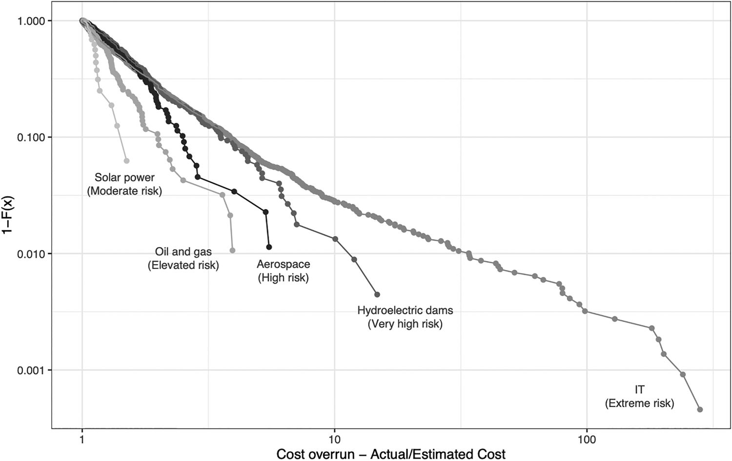
Complementary cumulative distribution functions (CDF) for selected cost risk profiles for each risk category in Table 4.
Discussion
In the Explanations section, we argued that the extant literature may be read as a theory of IT cost risk, which holds that immaturity, intangibility, goal ambiguity, and stakeholder resistance are attributes of IT projects that make them more risky than other project types in terms of cost. The higher the degree of immaturity, intangibility, goal ambiguity, and stakeholder resistance in a project, the more risky it will be. IT projects have more of all four attributes simultaneously than other project types. This is why IT is more risky, or so the theory claims. We emphasized, however, that the claim was unsupported by systematic data, because existing samples are too small to document, beyond statistical doubt, that IT projects are indeed more risky in terms of cost than other project types. With the present study, such doubt has been eliminated for the first time. Our data show that IT projects are, in fact, uniquely more risky than other project types in terms of cost, with IT being the only project type with an infinite mean for cost overrun (α ≤ 1) and thus infinite cost risk. With this finding, systematic data statistically support the theory expressed in the extant literature, but without proving it. Final proof would require further study.
Our study is an observational study (as opposed to a lab experiment or a randomized controlled trial). Final causality can, therefore, not be established. We consider, however, that with the systematic test of the theory shown in Figure 1, we have established a degree of what Pearl and Mackenzie (2019, p. 150) call “provisional causality,” which is causality contingent on the set of assumptions we have made and on the extensive controls for confounding variables and spurious effects. As emphasized by Pearl and Mackenzie, it is important not to treat observational studies like “second-class citizens” (op. cit.). Such studies have the advantage of being conducted in the actual habitat of the target population instead of in an artificial lab setting, and they can be “pure” in the sense of not being contaminated by issues of feasibility or bias in lab codes, according to Pearl and Mackenzie.
Our data have more to say about possible causes of extreme IT cost risk, however, than what is covered in the extant literature and Figure 1. First, we observe that in Figure 2, IT projects cluster with nuclear storage, defense, and the Olympics at the top of the diagram. These four project types have the lowest α values of all types, indicating the most extreme, fat-tailed cost risk. In contrast, at the bottom of the figure, solar power, energy transmission, nuclear decommissioning, and wind power cluster together with the highest α values—all larger than 4—indicating low, thin-tailed cost risk. Importantly, we observe there is no overlap between the 95% confidence intervals between the two groups, showing the groups are statistically significantly different in terms of cost risk. We further observe that the projects in the IT cluster at the top of Figure 2 are all projects with a high degree of bespokeness. In contrast, projects in the solar power cluster, at the bottom of the figure, are projects with a high degree of modularity, perhaps with the exception of nuclear decommissioning, which needs further study due to a too small sample, as noted above.
IT systems, nuclear storage, defense, and the Olympics are known for being tailor-made for each occasion, treating every project as a unique endeavor, with uniqueness being a known driver of extreme risk (Flyvbjerg et al., 2025). The opposite of bespokeness is modularity, which is part of the solution to the issue of extreme cost risk, including for IT. As a thought experiment, imagine what would have happened if solar, wind, and transmission projects had not been exposed to modularity. Would cost risk have been the same as for nonmodular projects, for example, IT and defense? If so, this would be a strong indication that the degree of modularity (from fully bespoke to fully modular) is a real causal variable for cost risk, according to Pearl and Mackenzie (2019, p. 155). The thought experiment is easy to imagine and substantiate because wind power and other modular projects, in fact, used to be nonmodular. Wind turbines were originally built one by one on construction sites, like buildings, with poor performance in terms of time and cost, like buildings. Eventually, construction sites were transformed into assembly sites, with the parts of wind turbines produced in modular fashion in manufacturing plants, brought on-site only for quick assembly. This helped bring time and cost under control, making wind competitive with other energy sources, resulting in a global boom for the industry. Modularity, therefore, seems to be a real cause of driving down cost risk, although other causes undoubtedly exist that warrant further research.
Of more direct relevance to IT projects, consider the Apple App Store. Apps on the App Store follow a modular design made mandatory by Apple. And not only that—App developers must use tools made by Apple that are also modular and mandatory. This is double modularity. Apple does not release transparent numbers, but by all accounts, the App Store is not only huge but also hugely successful, with millions of apps, billions of downloads, and hundreds of billions of dollars in revenues. The App Store is “big built from small” (Flyvbjerg & Gardner, 2023, p. 127), just like wind and solar farms. This has de-risked the App Store, unlike conventional bespoke IT, which may be considered key to the App Store’s—and Apple’s—success. If someone wanted to tame the risk on their IT projects —which the data show more people should do—then looking to the App Store and modularity for solutions would be a good place to start.
Second, our data also have more to say about project duration. The mean duration of IT projects is 3.2 years. The mean duration for all other project types is 6.9 years, that is, 2.2 times longer than IT. For the other three project types in the IT cluster at the top of Figure 1 (nuclear storage, defense, the Olympics), the difference is even larger. At least two interpretations are relevant in terms of cost risk. First, the longer a project takes, the more risky it will be, other things being equal, because variance grows with time and variance is risk. Based on this reasoning, IT projects should be among the least risky of the 23 project types in terms of cost risk, other things being equal. But the opposite is true. IT is the most risky. Said differently, for whatever reason, IT project planners and managers have very clearly been unable to translate the advantage of short duration into lower risk. If we corrected for this advantage by assuming IT projects take as long as the other project types, IT would be even more risky than it is, emphasizing just how uniquely extreme IT cost risk is. Project duration, therefore, does not directly explain IT cost risk but only indirectly in the sense that IT would be even more risky were it not for the short duration of IT projects, other things being equal. According to this line of reasoning, other variables annul the positive effect of the short duration for IT, and such variables—possibly the variables in the theoretical model in Figure 1—are probably stronger for IT than for other project types in explaining extreme cost risk.
In a different interpretation of project duration, other things are no longer equal, in the sense that the short duration of IT projects is now seen as an indication of more risk instead of less, because IT projects are possibly rushed through planning and delivery without proper preparation. This is not only the case for agile projects, where such rush is the point, but for all IT projects, on average, resulting in fast thinking, in Kahneman’s (2011) terms. Behavioral scientists have long established that fast thinking leads to behavioral bias, higher risk, and underperformance in decision-making. To the extent that IT is more rushed and more subject to fast thinking during decision-making than other project types, this would, therefore, account well for the observed data, with IT as the poorest performer of all types.
In sum, the data indicate we should possibly add bespokeness and fast thinking as two supplemental explanatory variables of extreme IT project risk in addition to the four variables shown in Figure 1. Further research is recommended to test the soundness of this conclusion.
Further Research
Another area for further research would be how to develop methods for systematically and precisely measuring the variables in the causal model—for example, immaturity and intangibility—and correlate such measures with cost risk. This would likely allow firmer conclusions regarding causality.
A second obvious area for additional research would be conducting analyses similar to those presented above but for benefit risk and schedule risk. As mentioned, we already did preliminary analyses of these, finding results similar to those found for cost risk, that is, fat tails. However, more data are needed together with more extensive analyses to arrive at firm conclusions for benefit risk and schedule risk. Additional data would also be desirable for cost risk for those project types that have small samples such as nuclear decommissioning, dams, and nuclear storage. For some project types, for example, the Olympics, which are hosted only every four years, establishing large samples will be impossible or difficult. But ideally, we would like a sample minimum of 100 projects for each project type, and preferably more for fat-tailed projects, because large samples are essential for those to arrive at reliable statistics, as explained above. Adding further project types—beyond the 23 included here—would also be an area for further research. We are working in all these areas, constantly expanding the database. Finally, other scholars should independently try to replicate our study, based on their own independently collected large samples of data.
Third, further research on generative mechanisms for fat tails is particularly pertinent. Now that we know most project types have fat-tailed risk, we should focus directly on this fact and try to explain tails in terms of the specific mechanisms that generate fat tails. Key thinkers on fat tails are Benoit Mandelbrot and Nassim Nicholas Taleb. Their works will, therefore, have to become part of the canon of project management scholarship. Mandelbrot (1997, p. 48) observed that explanations of fat tails seem to work in physics, because here “many instances of scaling are well-understood,” whereas “only a few instances of scaling in the social sciences led to convincing explanations.” That is still the situation today. Project management scholarship is social science, obviously, because it is about human behavior. So, we have a special challenge compared with natural science, according to Mandelbrot. Nevertheless, we may seek inspiration from natural science, which has shown that convexity is key to explanations of fat tails (Taleb, 2020). Social science needs social explanations, so key questions will be: What is convexity in social explanations, and what drives it? From behavioral science, we know that behavioral bias drives amplification and that amplification drives convexity. Thus, behavioral bias—both cognitive bias and power bias (Flyvbjerg, 2021)—will likely be a productive place to start with research on generative mechanisms, including for the uniquely fat tail of IT cost risk documented above. We consider this a particularly interesting area for further research.
Finally, the present study provides a cross-group comparison of IT cost risk with other project types. Flyvbjerg et al. (2022) provided a within-group analysis of IT projects, but without distinguishing between different subtypes of IT projects. We propose, as a logical next step, to conduct a study of intragroup variation between different subtypes of IT project regarding cost risk, to establish possible differences between subtypes.
Conclusions
In conclusion, the present article conducts a cross-group comparison of IT cost risk versus 22 other project types. The article documents, for the first time, that IT projects have higher cost risk than any other project type. Uniquely, IT is the only project type with a Pareto 1 tail parameter (α) smaller than one, meaning that cost risk is so fat-tailed that the mean and variance of the risk distribution are infinite, leaving IT cost risk infinite and unpredictable. Conventional forecasting, therefore, simply does not work for IT cost. Cost risk for the other 22 project types also follows the Pareto 1 but with less fat tails, indicated by α values larger than one.
The article further supports, without final proof, the theory in the extant literature that claims immaturity, intangibility, goal ambiguity, and stakeholder resistance to be causes of extreme IT risk. Thus far, this theory has been statistically unsupported in the literature. The present article supports the claims for the first time. The claims may, therefore, possibly explain the unique extremity of IT cost risk that we have documented. We add two further explanations of extreme IT risk, directly grounded in our data and analyses: the bespokeness of IT projects (as opposed to standardized modularity) and the “think fast” nature of IT (as opposed to “think slow” à la Kahneman). Finally, we suggest areas for further research, focusing on generative mechanisms for fat tails.
Footnotes
Notes
Author Biographies
Appendix A. Literature Review
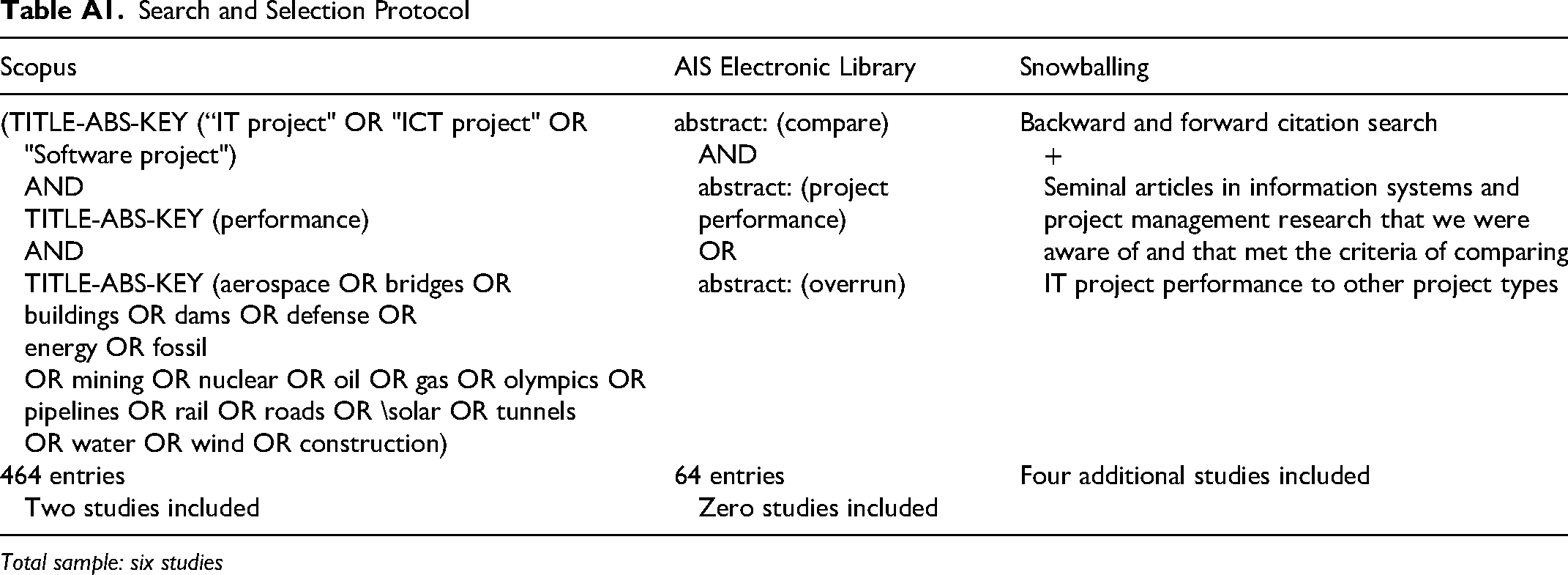
Our literature review followed the guidelines offered by Webster and Watson (2002). The goal was to identify articles that focus on comparing the performance of IT with other project types. To do so, we conducted a systematic search in the Scopus database for research articles, conference papers, and book chapters using three sets of keywords: “IT project/ICT project/Software project,” “performance,” and an extensive list of various project types and domains (see Table A1 for the complete search string). This search yielded 464 entries, of which two were deemed relevant to be included in the final sample. In addition, to check and extend our coverage within the IS literature, we searched the AIS Electronic Library (an IS-specific database) using a broader set of search keywords: “compare” and “project performance” or “overrun.” This provided 64 additional entries, but none was deemed relevant for inclusion in the final sample. For both searches, we initially screened the returned entries based on title and abstract. Finally, we conducted supplementary snowball sampling through backward and forward citation searches and by reviewing additional seminal articles in information systems and project management research that we were aware of. We also added articles that met the criteria of comparing IT project performance to other project types. This yielded four additional articles in the final sample. Search and Selection Protocol
Total sample: six studies
Scopus
AIS Electronic Library
Snowballing
(TITLE-ABS-KEY (“IT project" OR "ICT project" OR "Software project")
AND
TITLE-ABS-KEY (performance)
AND
TITLE-ABS-KEY (aerospace OR bridges OR
buildings OR dams OR defense OR
energy OR fossil
OR mining OR nuclear OR oil OR gas OR olympics OR
pipelines OR rail OR roads OR \solar OR tunnels
OR water OR wind OR construction)abstract: (compare)
AND
abstract: (project performance)
OR
abstract: (overrun)Backward and forward citation search
+
Seminal articles in information systems and project management research that we were aware of and that met the criteria of comparing IT project performance to other project types
464 entries
Two studies included64 entries
Zero studies includedFour additional studies included
In total, our search and selection processes provided a list of six articles, with the earliest study published in 2008 and the most recent in 2022. We included studies that explicitly provided and compared project performance data (measured in terms of cost, delays, or benefits) between IT projects and at least one other type of project. We also included two studies comparing the importance of various factors impacting project performance in IT compared with other project types.
As summarized in Table A2, we analyzed each article to identify (1) which project type(s) IT was compared with, (2) the type of data, and (3) key findings concerning if and how IT projects are different. Included Studies that Compared IT Projects to Other Project Types IT projects Construction Change management IT Green energy Nanotechnology Communication IT Construction IT projects Construction IT Construction IT Communication Construction Engineering Government Production Service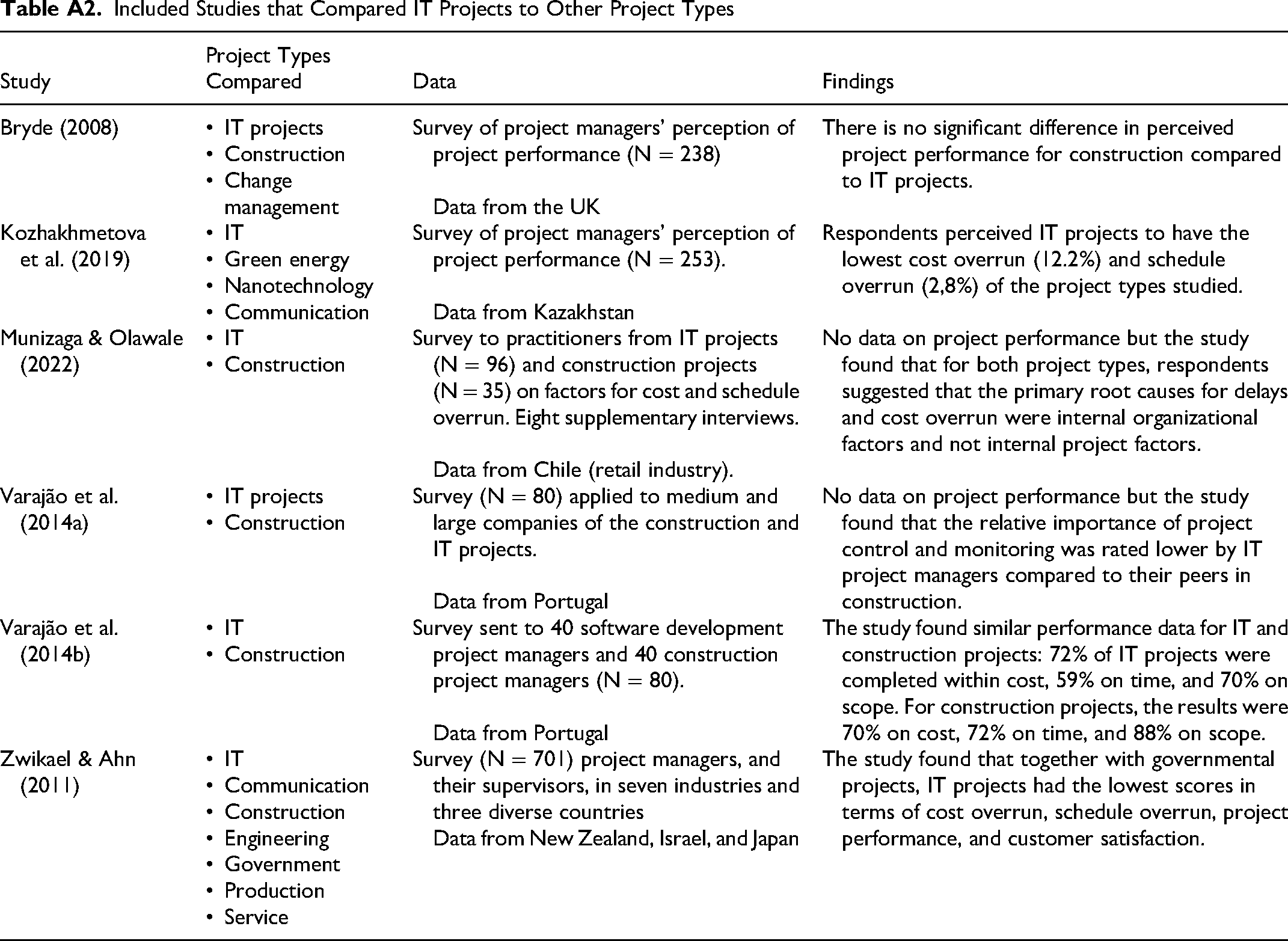
Study
Project Types Compared
Data
Findings
Bryde (2008)
Survey of project managers’ perception of project performance (N = 238)
Data from the UKThere is no significant difference in perceived project performance for construction compared to IT projects.
Kozhakhmetova et al. (2019)
Survey of project managers’ perception of project performance (N = 253).
Data from KazakhstanRespondents perceived IT projects to have the lowest cost overrun (12.2%) and schedule overrun (2,8%) of the project types studied.
Munizaga & Olawale (2022)
Survey to practitioners from IT projects
(N = 96) and construction projects
(N = 35) on factors for cost and schedule overrun. Eight supplementary interviews.
Data from Chile (retail industry).No data on project performance but the study found that for both project types, respondents suggested that the primary root causes for delays and cost overrun were internal organizational factors and not internal project factors.
Varajão et al. (2014a)
Survey (N = 80) applied to medium and large companies of the construction and IT projects.
Data from PortugalNo data on project performance but the study found that the relative importance of project control and monitoring was rated lower by IT project managers compared to their peers in construction.
Varajão et al. (2014b)
Survey sent to 40 software development project managers and 40 construction project managers (N = 80).
Data from PortugalThe study found similar performance data for IT and construction projects: 72% of IT projects were completed within cost, 59% on time, and 70% on scope. For construction projects, the results were 70% on cost, 72% on time, and 88% on scope.
Zwikael & Ahn (2011)
Survey (N = 701) project managers, and their supervisors, in seven industries and three diverse countries
Data from New Zealand, Israel, and JapanThe study found that together with governmental projects, IT projects had the lowest scores in terms of cost overrun, schedule overrun, project performance, and customer satisfaction.
The studies are predominantly based on survey data produced by asking project managers how they perceived project performance within their project type and asking to rate the importance of various factors in their industry (Bryde, 2008; Kozhakhmetova et al., 2019; Munizaga & Olawale, 2022; Varajão et al., 2014a; Zwikael & Ahn, 2011). Three studies compared two project types (IT and construction), and three studies compared IT to multiple project types. However, none of the studies explained how they categorized their project types, making it difficult to compare results within and across studies. Furthermore, the studies tend to have small sample sizes and to be limited to a single country.
Specifically, Kozhakhmetova et al. (2019) compared green energy projects with nanotechnology projects, communications projects, and IT projects. This study is based on 253 questionnaires, of which 71 involved IT projects. The average cost overrun for IT was found to be 12.2%, which was less than for the other two project types. The study has several limitations, however. First, the sample size was relatively small. Getting an accurate picture of a fat-tailed distribution requires a larger sample than that used. Second, the research was based on a questionnaire, and cost overrun was subjectively assessed as a percentage based on a respondent’s recollection rather than on cost data documented by high-quality written records.
The Munizaga and Olawale (2022) study compared possible factors that contribute to cost overruns in IT projects and construction projects in the retail industry in Chile. Their study involved questionnaires, which were completed by 96 respondents for IT projects and 35 respondents for construction projects. They did not find significant differences between these two project types in terms of the factors perceived to cause cost overruns. However, they did not report any findings regarding the actual cost overruns for the two types of project. Thus, based on what they reported, we cannot conclude that project type doesn’t matter when it comes to cost overruns. Furthermore, their sample size was small and, again, fat-tailed distributions require large samples.
In sum, our review revealed that there has been no attempt to empirically examine if and how IT projects perform differently compared to other project types through objective performance measures (e.g., cost overrun, schedule overrun, and benefit realization) at a large scale.
Appendix B. Data Collection
The sample used in the present study includes 11,011 projects across the 23 project types listed in Appendix C, at a total value of US$4.64 trillion in 2023 prices. Geographically, the projects are located in 126 countries on six continents. Historically, the data cover the period from 1781 to 2021, with the majority of projects going live recently, in the 21st century. The average project size ranges from US$29 million to US$16 billion in 2020 prices. Average project duration varies from one to 14 years, measured from the final investment decision to going live. The data cover both government and business projects.
Data on estimated and actual costs of projects are generally difficult to obtain. No statistical agency or other data service exists from which valid and reliable data may be secured. Over more than 20 years, the principal author and his associates have, therefore, mined such data and developed their own dataset, the largest of its kind. Data collection began with projects in transportation infrastructure, following a methodology pioneered by Pickrell (1990) in his classic study of forecast versus actual cost and utilization in U.S. urban rail transit projects. Pickrell systematized ideas first employed by Hamer (1976). Pickrell rigorously measured estimated and actual costs and benefits in 10 transit projects and insisted that the estimates to be compared to actual outcomes were those on the basis of which planners and officials had decided to proceed with proposed projects. Pickrell argued that revisionist forecasts issued by planners and officials later in the planning and tendering process or after construction had commenced—in short, after an irrevocable commitment to proceed with the project had been made—were irrelevant, and comparing them to subsequent actual outcomes, as was (and is) common, was misleading because later forecasts did not influence the decision to proceed with the project. The methodology followed by Pickrell has since become an international standard for collecting and comparing data on estimated and actual costs (and benefits) in capital investing.
Like Pickrell, we collected data on both costs and benefits. Here, we focus on costs (for a study covering both costs and benefits, see Flyvbjerg & Bester, 2021). Our first dataset was published in Flyvbjerg et al. (2002, 2005), covering 258 transportation capital projects. This was the first time an academic dataset was large enough to allow statistically valid conclusions regarding cost risk and the accuracy of cost estimates in transportation capital projects. Since then, we have expanded the dataset to cover more project types. The present study covers 23 types in total. Over two decades, we have continuously grown the dataset from three sources. First, we collected our own data directly from project owners, for which data were available both when the projects were decided (estimated cost) and later completed (actual cost). Second, we used freedom of information acts (FOIA) to access data. Third, to allow meta-analysis, we included data from other researchers in other studies who had done the data collection, for example, for auditor reports, official reports, and academic research.
At first, collecting data directly from owners proved difficult and slow. However, at one stage, we decided to offer our data to owners to benchmark their projects on the condition they give us access to their data for use in our research after proper anonymization and signing of nondisclosure agreements. From that point on, data collection became easier and faster. For all sources, we used formal and informal searches. We did (and do) formal bibliographic searches on a continuous basis using Web of Science, Google Scholar, and individual journals. In addition, our professional network informally kept (and keeps) us informed about new projects and new studies with relevant data. Finally, after the publication of our 2002 and 2005 studies, these and later research became so widely cited that we were able to reliably discover new studies with new data simply by tracking who cited our publications, which therefore became a key part of our systematic bibliographic searches. For increased accuracy, we triangulated the formal and informal searches against each other. We deem that all projects and all studies for which valid and reliable data on estimated and actual cost are publicly available have been considered for inclusion in our dataset for the project types covered by the study. On that basis, we consider it unlikely that important public data exist that are not included or were not considered for inclusion.
Whether data were collected by us or by other researchers, they typically originated from annual or other regular accounts, cost and procurement records, revenue accounts, and auditors’ data. 15 Only data that could be supported by reliable documentary evidence were included to avoid well-known problems with recalled data and interviewee biases. Even so, substantial amounts of data had to be rejected due to insufficient data quality, amounting to approximately 25% of all cost data (compared with 50% for benefit data). Common reasons for data rejection were lack of clarity regarding (1) baselines (not knowing the year for which data apply and from which overrun was calculated), (2) price levels (not knowing in which year's prices the monetary values were calculated), (3) exchange rates (not knowing the basket of exchange rates used to convert local currencies into U.S. dollars), and (4) discount rates and price indices (not knowing how monetary values were conflated over time). Datasets were also rejected for which outliers had been omitted for no good reason or for which such omission was clearly statistically unsound (see further Flyvbjerg et al., 2018). For studies done by others, data were checked for validity and reliability as well as for duplication to avoid double counting. If data were already included in our dataset, or if they were not valid and reliable, they were left out. After rejecting data in this manner, data on cost overrun were available for 11,011 projects, of which 2,845 were directly from owners, 2,653 from FOIA requests, 4,141 from publicly available data, and 1,372 from academic publications. The inclusion of data from different sources made it possible to statistically test whether project performance varied with data sources, which was found not to be the case, which corroborates the robustness of results across sources. Specifically for the IT project data, we found no statistically significant differences between data sources (Flyvbjerg et al., 2022), which is important because differences in variance may spuriously generate fat tails, which would then be an artifact of error in data collection, instead of being a characteristic of the data. This error has been tested for.
We also did not find any historical trends of improving or deteriorating project performance (p = 0.468, linear regression log-transformed cost overrun), which again suggests that the fat tails of IT data are not spuriously caused by including data with different variances.
As a final robustness check, we found that the size of projects, measured by estimated duration and cost, was not statistically significantly associated with cost overrun (p = 0.231 for duration, p = 0.06 for cost). The p value for cost is close to the level of statistical significance of 0.05, but one should note that a significant relationship may be expected because cost overrun is calculated as actual divided by estimated cost and, therefore, correlated. This finding tells us that the cost overruns observed in the data are not a result of the varying sizes of IT projects. We may, therefore, compare IT with other project types across the entire size range.
Finally, it should be mentioned that, recently, it was discovered that some ex-post studies of cost forecasting have been contaminated by significant statistical errors, for instance, in pooling data with incompatible baselines and excluding outliers that should have been included. Such studies cannot be trusted and cannot be replicated. The same holds for meta-studies that include these studies without being aware of their shortcomings. This unhappy situation—which signifies the arrival of junk science in capital project scholarship—is accounted for by Flyvbjerg et al. (2018, 2019), together with recommendations for how to mitigate the problem. The importance of rooting out studies with faulty data from the body of work in project scholarship cannot be overemphasized if the field wants to enjoy continued credence in the academy, policy making, and with the general public. Data from studies that proved contaminated were not included in the present research.
Preferably, costs would be measured over the full life cycle of a project. However, such data are rarely, if ever, available. Convention is, therefore, to measure the cost of projects by the proxy of up-front capital costs to deliver the project and bring it online. This convention is followed here. Estimated costs are the estimates made at the time of the final investment decision, or FID, based on the final business case, which is the baseline in time from which cost overrun is measured. Actual costs are measured as recorded outturn costs.
Projects were included in the sample based on data availability, as mentioned. This means that the results of the statistical analyses presented in the main text are probably conservative. In other words, it is likely that cost overruns within the project population are even greater than those captured by our sample. This is because the availability of data is often an indication of better-than-average project management and because data from badly performing projects are often not released and are, therefore, likely to be underrepresented in the sample. This must be kept in mind when interpreting results. For more on data collection and selection bias, see Flyvbjerg (2005, 2016) and Flyvbjerg et al. (2002, 2005, 2022).
Appendix C. Project Types and Sample Sizes
Table C1 lists the definitions and sample sizes for the total sample of projects (for N > 10) and for projects with cost overrun (A/E > 1). The typology of projects was derived from previous studies of overrun in their respective fields. This study is the first to compare overrun data across different project types and sectors, as mentioned in Appendix A. Energy projects follow the classification used by Sovacool et al. (2014) that differentiates projects by fuel type. Transportation infrastructure follows the conventional classification by transport mode used by Flyvbjerg et al. (2003). Dams follow the classification used by Ansar et al. (2014). We separated buildings as a special case of construction as per the convention of Engineering News-Record (ENR, n.d.). Project Types and Sample Sizes, N = 11,011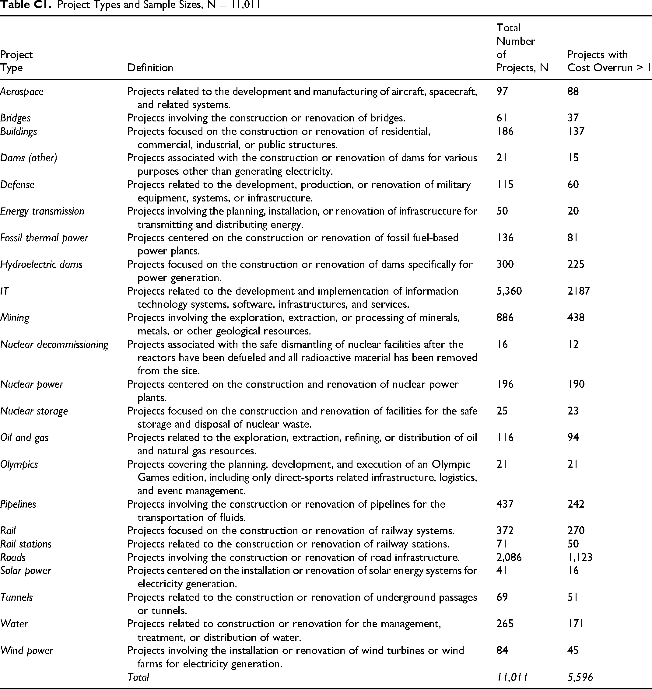
Project
Definition
Total
Projects with
Cost Overrun > 1
Aerospace
Projects related to the development and manufacturing of aircraft, spacecraft, and related systems.
97
88
Bridges
Projects involving the construction or renovation of bridges.
61
37
Buildings
Projects focused on the construction or renovation of residential, commercial, industrial, or public structures.
186
137
Dams (other)
Projects associated with the construction or renovation of dams for various purposes other than generating electricity.
21
15
Defense
Projects related to the development, production, or renovation of military equipment, systems, or infrastructure.
115
60
Energy
transmission
Projects involving the planning, installation, or renovation of infrastructure for transmitting and distributing energy.
50
20
Fossil thermal power
Projects centered on the construction or renovation of fossil fuel-based power plants.
136
81
Hydroelectric dams
Projects focused on the construction or renovation of dams specifically for power generation.
300
225
IT
Projects related to the development and implementation of information technology systems, software, infrastructures, and services.
5,360
2187
Mining
Projects involving the exploration, extraction, or processing of minerals, metals, or other geological resources.
886
438
Nuclear decommissioning
Projects associated with the safe dismantling of nuclear facilities after the reactors have been defueled and all radioactive material has been removed from the site.
16
12
Nuclear power
Projects centered on the construction and renovation of nuclear power plants.
196
190
Nuclear
storage
Projects focused on the construction and renovation of facilities for the safe storage and disposal of nuclear waste.
25
23
Oil and gas
Projects related to the exploration, extraction, refining, or distribution of oil and natural gas resources.
116
94
Olympics
Projects covering the planning, development, and execution of an Olympic Games edition, including only direct-sports related infrastructure, logistics, and event management.
21
21
Pipelines
Projects involving the construction or renovation of pipelines for the transportation of fluids.
437
242
Rail
Projects focused on the construction or renovation of railway systems.
372
270
Rail stations
Projects related to the construction or renovation of railway stations.
71
50
Roads
Projects involving the construction or renovation of road infrastructure.
2,086
1,123
Solar power
Projects centered on the installation or renovation of solar energy systems for electricity generation.
41
16
Tunnels
Projects related to the construction or renovation of underground passages or tunnels.
69
51
Water
Projects related to construction or renovation for the management, treatment, or distribution of water.
265
171
Wind power
Projects involving the installation or renovation of wind turbines or wind farms for electricity generation.
84
45
Total
11,011
5,596
Appendix D. Data Analysis and Robustness Checks
Here, we account for how we fit probability distributions to the data for each project type in three steps:
1. Visual inspection of probability distributions for each project type;
2. Pareto and lognormal goodness of fit-tests; and
3. Bootstrap analysis of α values.