Evaluating liquefaction exposure of road networks to support decision-making

Abstract

This article discusses different approaches to evaluate liquefaction exposure across road networks and inform decision-making processes regarding asset management, emergency preparation and response planning. Using the New Zealand State Highway network, liquefaction exposure is assessed based on ground shaking from two sources: (1) various return period shaking intensities from the National Seismic Hazard Model and (2) a suite of specific earthquake scenarios. The first approach considers the likelihood of liquefaction exposure at each location conditional on different levels of ground shaking, suitable for assessing individual network components. The second approach presents liquefaction exposure for a specific earthquake scenario, capturing the extent of exposure across a network. In addition, it offers a new indicator, the number of events (NoE), identifying network sections that could be affected by liquefaction manifestation across multiple earthquake scenarios. For both approaches, the extent of potential exposure (number of affected 100 m-segments) and the level of network disruption (number of affected links representing segments between intersections) are estimated at both national and regional scales. While the national-scale assessment helps to quantify liquefaction exposure across the entire network, providing valuable insight for asset management, the regional-scale assessments identify potential worst-case scenarios, identify locations affected by multiple events and allow for more informed emergency management decision-making. Future research should expand the multi-scenario approach, incorporate network related aspects, such as criticality or redundancy, and consider recurrence intervals for scenario weighting or perform a full probabilistic liquefaction hazard analysis to enhance the evaluation of potential impacts and to further support decision-making.

Introduction

Liquefaction and lateral spreading can severely impact road networks, including surface cracking, deformation, and lateral displacement, and may require extensive resources to repair damage and restore network services. In addition, the potential disruption of transport services can interfere with emergency response efforts, considering that road networks are essential for providing access to critical facilities, such as hospitals. Events such as the 1964 Niigata, Japan, earthquake (Kawakami and Asada, 1966), the 1989 Loma Prieta, California, earthquake (Seed et al., 1991) or the 2011 Christchurch, New Zealand, earthquake (Cubrinovski et al., 2012) have demonstrated the social and economic consequences of transport network disruptions caused by liquefaction and lateral spreading, emphasizing the need to better understand liquefaction hazards across road networks.

Various studies have assessed liquefaction hazards across road networks at a regional scale. Lu et al. (2024) estimated liquefaction risk across an urban area in Taiwan by integrating a geotechnical database, which included borehole and soil testing data, with empirical models to quantify road vulnerability. D’Apuzzo et al. (2022) applied a geostatistical approach, combining probabilistic seismic hazard models and permanent ground deformation analysis to assess road damage and its socio-economic consequences in a district of northern Italy. Kajihara et al. (2020) developed an empirical relationship between the Liquefaction Potential (LP) and observed road subsidence using LiDAR data and borehole logs.

These studies rely on geotechnical data, such as cone penetration test (CPT) records, to characterize subsurface conditions. However, due to the time- and cost-intensive nature of site investigations, those approaches are typically not practical for large-scale assessments. As an alternative, geospatial liquefaction models can be used, which estimate surface manifestation based on broadly available datasets. While these models have limitations due to their simplified representation of subsurface conditions, they offer a more time- and cost-efficient solution (Maurer, 2018). Despite their advantages, a comprehensive large-scale liquefaction assessment of road networks has not yet been conducted.

This article addresses that gap by providing a national-scale evaluation of liquefaction exposure across roads. Incorporating both recurrence-based and scenario-based ground shaking estimates, this study aims to inform decision-making processes regarding asset management as well as emergency preparation and response planning. Using the New Zealand State Highway network as a case study, liquefaction exposure is evaluated based on the liquefaction probability calculated by a region-specific geospatial liquefaction model for ground shaking data derived from two sources: (1) return period shaking intensities from the National Seismic Hazard Model and (2) a suite of specific earthquake scenarios. Return period shaking intensities offer valuable insight into the likelihood of a specific ground shaking level at each location conditional on different levels of ground shaking. This approach is often used at the component or project scale, where stakeholders such as engineers rely on these estimates to inform design and compliance with engineering standards. However, return period assessments fail to capture the spatial characteristics and extent of liquefaction for a single earthquake scenario. Evaluating a wide range of individual events addresses this limitation and provides insight into the exposure of the wider network by identifying sections that could be repeatedly affected by liquefaction manifestation, as well as scenarios that could impact multiple parts of the network. This article does not intend to directly compare the return period and earthquake scenario estimates as equivalent measures of liquefaction exposure, but rather to present them as complementary perspectives. Furthermore, this study does not aim to perform a full probabilistic analysis, but to provide a better understanding of the strengths and limitations of the two approaches, with a focus on how the exposure results can be interpreted to support decision-making. While a probabilistic liquefaction hazard analysis may offer additional insight, particularly for stakeholders prioritizing risk-based estimates, the limitations of the geospatial model used in this study, including its simplified nature and lack of site-specific geotechnical data, reduce its suitability for detailed risk assessments. For this reason, this study follows a more simplified approach, focusing on the geographic extent and consequences of potential disruptions, rather than their likelihood.

For both approaches, the number of State Highway segments (100 m) and links (segments between intersections) predicted to experience liquefaction manifestation are calculated, quantifying the extent of potential exposure and the level of network disruption caused by liquefaction manifestation. Results are compared on multiple scales: While national-scale assessments provide valuable information for asset management, such as infrastructure investments, regional-scale assessments identify events of particular interest, such as worst-case scenarios, and allow for more informed decision-making regarding emergency management. For the assessment involving a suite of earthquake scenarios, the number of events (NoE) predicted to result in liquefaction manifestation is used as an additional indicator to quantify and compare exposure. Limitations and uncertainties are discussed, focusing on questions and challenges that can be addressed in future research.

Data and methodology

This section describes the framework for estimating and evaluating liquefaction exposure across the New Zealand State Highway network. It includes the geospatial model used to calculate the liquefaction probability, the tools for estimating ground shaking intensities, and the approach for converting linear network data into points to define locations where liquefaction exposure is assessed.

Liquefaction model

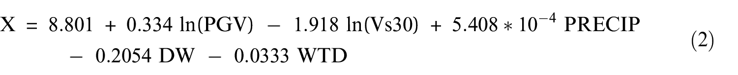
The liquefaction probability is calculated using a modified version of the geospatial liquefaction model developed by Zhu et al. (2017), which is globally applicable and has been implemented in hazard tools, such as the US Geological Survey ground failure product (Allstadt et al., 2021). Based on logistic regression, Zhu et al. (2017) correlated observational data from 27 earthquakes with geospatial data on soil properties associated with liquefaction manifestation. Their research indicated that a combination of peak ground velocity (PGV) in cm/s, shear wave velocity in the upper 30 m (Vs30) in m/s, annual precipitation (PRECIP) in mm, distance to the closest water body (DW) in km and water table depth (WTD) in meters below ground level (m. b. g. l.) leads to the highest prediction performance. The liquefaction probability (P) is calculated by the equation:

$$\mathrm{P}=1/(1+\exp (-\mathrm{X}))$$

(1)

where X equals a function of the explanatory variables:

$$\begin{array}{c}\multicolumn{1}{c}{\mathrm{X}=8.801+0.334\ln (\mathrm{PGV})-1.918\ln (\mathrm{Vs}30)+5.408*{10}^{-4}\mathrm{PRECIP}}\\ \multicolumn{1}{c}{-0.2054\mathrm{DW}-0.0333\mathrm{WTD}}\end{array}$$

(2)

The liquefaction probability describes the likelihood of liquefaction manifestation in a specific location; however, it fails to predict the liquefaction type (e.g. cracking vs lateral spreading) or severity (e.g. minor vs severe) as it does not account for subsurface soil properties or site-specific deformation mechanisms.

It is assumed that no liquefaction manifestation occurs (P = 0) for the following conditions (Rashidian and Baise, 2020; Zhu et al., 2017):

• PGV < 3 cm/s;

• PGA < 0.1 g;

• Vs30 > 620 m/s.

In addition, PRECIP is restricted to a maximum of 1700 mm to reduce overprediction in areas with high rainfall. Rashidian and Baise (2020) recommended this threshold as it represents the upper quartile of the precipitation values used to train the liquefaction model by Zhu et al. (2017). They found that regions above this threshold tend to overestimate the liquefaction spatial extent (area predicted to experience liquefaction based on P). This adjustment is relevant to the study area, as the West Coast of the South Island presents annual rainfall of approximately 2000 mm in low-elevation coastal locations and 10,000 mm and above in high elevations (Macara, 2016).

Rashidian and Baise (2020) also suggested an optional earthquake magnitude scaling factor (MSF) for the PGV term in order to reduce overprediction for low-magnitude events. This study does not apply the MSF for multiple reasons: First, the MSF has the greatest effect on earthquakes below M6; very few events assessed in this article have M < 6 and these did not result in predictions of liquefaction manifestation due to the PGV condition (P = 0 for PGV < 3 cm/s). It should be noted that this circumstance is specific to the events chosen in this study; while M < 6 events can generate PGV values above 3 cm/s and potentially cause liquefaction manifestation, this was not the case for the events analyzed here. Second, while the MSF could also affect events with M ≥ 6, its impact is less prominent. Rashidian and Baise (2020) found that it did not significantly impact their findings. Finally, as Rashidian and Baise (2020) focused on the liquefaction spatial extent, it remains uncertain whether applying the MSF to a probability-based assessment (P) would be justified. Therefore, this study does not use the MSF, following a more conservative approach.

Previous research (Lin et al., 2021) modified the approach of Zhu et al. (2017) by replacing the global variables for Vs30, DW and WTD with New Zealand-specific datasets without changing the coefficients in Equation 2. Further details on the input variables of the geospatial liquefaction model are provided at the end of this article.

Evaluating the modified model for the 2010–2011 Canterbury Earthquake Sequence (Lin et al., 2021) and the 2016 Kaikōura earthquake (Lin et al., 2022) indicated improved prediction performance due to higher resolution (between 25 and 200 m) and/or more accurate information of the New Zealand-specific datasets. Results also suggested that liquefaction manifestation can be expected for a calculated liquefaction probability of 46% or above. As opposed to the continuous probability scale ranging from 0 to 1, this threshold allows for a binary prediction outcome. Although offering a simplified representation of the liquefaction hazard, the binary classification is appropriate given the scale of the analysis and the resolution of the input data. It provides a more practical basis for identifying which roads would experience liquefaction manifestation during an earthquake. Probabilities or abstract liquefaction levels (e.g. “low” to “high”), however, require additional interpretation by stakeholders, which may limit their practicality as they could result in inconsistent decision-making. Moreover, presenting varying degrees of liquefaction without underlying models to quantify the corresponding disruption across the network could give a misleading sense of precision and introduce further uncertainty.

Due to the use of geospatial data, the approach does not estimate the liquefaction severity, as this would require more site-specific information on the soil profile and the road construction characteristics. While indices based on subsurface data, such as the Liquefaction Potential Index (LPI) or the Liquefaction Severity Number (LSN), can represent the severity of manifestation and relate to the severity of damage across the road network, their availability is limited to specific regions. By prioritizing a simplified approach and focusing on a geospatial model, this study ensures practical applicability and consistency in assessing liquefaction exposure across the entire network.

In addition to the aforementioned conditions, the modified model incorporates another assumption based on the soil type (MBIE, 2017). No liquefaction is expected if

• The soil is classified as (late) Holocene age deposits and WTD ≥ 8 m.b.g.l. or,

• The soil is classified as late Pleistocene age deposits and WTD ≥ 4 m.b.g.l.

These thresholds are based on New Zealand guidelines for planning and building on liquefaction-prone land, suggesting that deeper water tables reduce the likelihood of liquefaction manifestation due to lower pore pressure development (MBIE, 2017). Late Holocene deposits are assumed to be more susceptible to liquefaction as they are often characterized by loose sediments, presenting a higher WTD threshold than late Pleistocene deposits, which are more consolidated, hence, less susceptible to liquefaction.

Figure 1 presents the liquefaction susceptibility map of New Zealand, generated using the values from Equation 2 without the ground shaking parameter (0.334 ln(PGV)). The “none” category describes areas where liquefaction is not expected following the soil condition by MBIE (2017). The other categories are adapted from Zhu et al. (2017) by converting susceptibility values into qualitative classes. This conversion was performed by aligning the susceptibility distribution with existing geology-based liquefaction susceptibility maps. However, due to the use of New Zealand-specific input data, the classification is skewed, resulting in only small areas being categorized as having low or very low susceptibility. Nonetheless, the map allows for the comparison of higher susceptibility categories, indicating maximum susceptibilities across the central area of the North Island (Figure 1a) and the West Coast of the South Island (Figure 1b). The susceptibility map helps to interpret the results of this article and will be referred to in subsequent sections.

Figure 1.

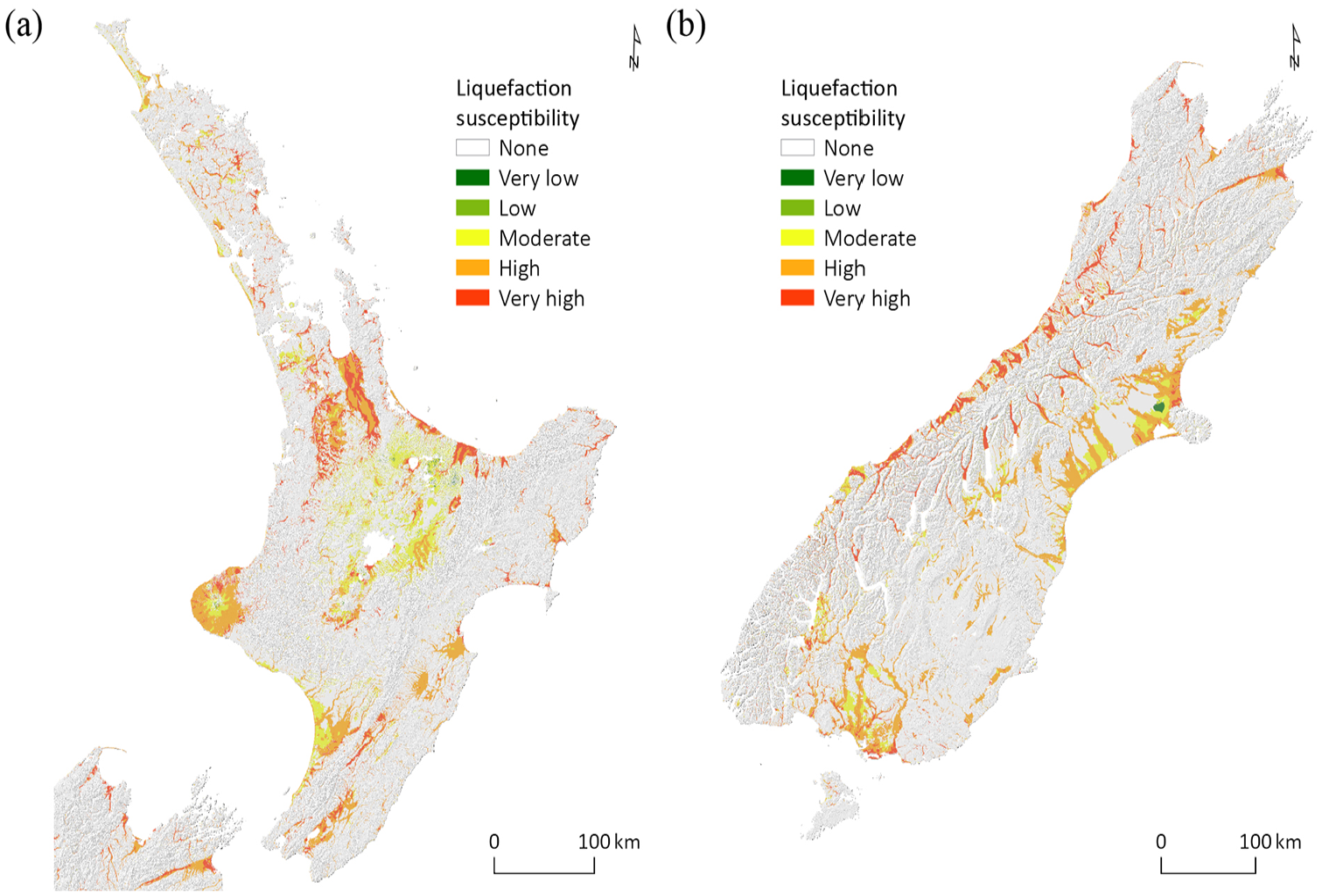
Liquefaction susceptibility for the (a) North Island and (b) South Island of New Zealand.

Ground shaking intensities

The ground shaking intensities for the different return periods are based on the hazard curves from the 2022 National Seismic Hazard model (NSHM), which uses geologic data and historical earthquake case studies to simulate the ground motions across a 10-km-grid spanning New Zealand (Gerstenberger et al., 2023). In total, 6 exceedance probabilities from the NSHM are considered in the assessment: 63%, 39%, 18%, 10%, 5%, and 2% in 50 years, which correspond to 50-, 101-, 252-, 475-, 975- and 2475-year return periods, respectively.

For each return period/exceedance probability, the weighted mean PGA values (in g) and spectral acceleration at a 0.5-second period (SA[0.5 s], in cm/s²) are retrieved from the NSHM. Vs30 data, which is directly used in ground motion characterization models to account for local site effects, is also used in the liquefaction model.

To meet the input requirements of the geospatial liquefaction model, which uses PGV to determine liquefaction probability (Equation 2), SA[0.5 s] is converted to PGV following the approach from Bommer and Alarcon (2006). This conversion involves adjusting the units of SA[0.5 s] from cm/s² to g (1 cm/s²≈ 0.001 g), which results in the equation:

$$\mathrm{PGV}=49\mathrm{SA}[0.5\mathrm{s}]$$

(3)

In addition to the return period intensities, ground shaking intensities for specific earthquake scenarios are generated using Cybershake New Zealand v19.5 (Bradley et al., 2020), a physics-based ground motion simulation tool. Unlike empirical models, Cybershake simulates seismic wave propagation and ground shaking from a wide range of earthquake rupture scenarios, including more than 200 fault sources. The simulations account for local site effects through physics-based modeling, incorporating basin effects and near-surface amplification, which differs from the Vs30-based site adjustments applied in the NSHM.

Among the over 10,000 simulated events, a set of 479 scenarios is investigated in this article. All scenarios represent single-rupture events, meaning each event corresponds to a rupture on a single fault rather than a multi-segment rupture. The selection is based on the availability of ground motion data for 536 events, which represent ruptures of known faults across New Zealand. As the aim of this study is to investigate and compare the geographic distribution and potential consequences of specific events, occurrence rates of the earthquake scenarios, which would shift the focus toward likelihood-weighted outcomes, are not incorporated.

The selected scenarios are further filtered based on the aforementioned condition that liquefaction manifestation requires a ground shaking intensity associated with a PGA of 0.1 g or above and a PGV of 3 cm/s or above in at least one location across the State Highway network. Figure 2a presents the surface projection of the corresponding faults including the moment magnitude (M_W). The majority are active shallow crustal ruptures with a maximum M_W of 8.2 (average M_W = 7.1) or describe shallow crustal earthquakes in volcanically active regions with a maximum M_W of 6.8 (average M_W = 6.4). While most crustal events are onshore and scattered across both the North and the South Island of New Zealand, all events in volcanic regions are restricted to the North Island. It is important to note that these events do not reflect all possible earthquake scenarios that could occur across New Zealand. Instead, they are selected to provide a representative sample of events to support the analysis and discussions presented in the following sections.

Figure 2.

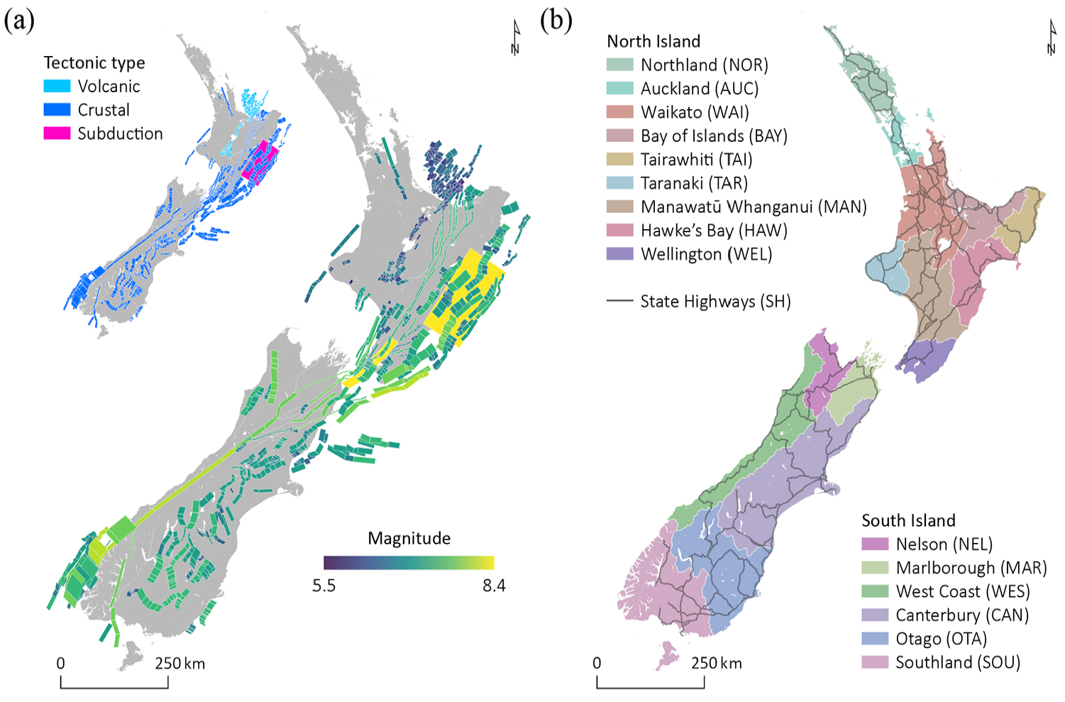
(a) Moment magnitude and tectonic type of the 479 fault ruptures used in the multi-scenario assessment. (b) Location of the 15 Civil Defense Emergency Management (CDEM) groups as well as the New Zealand State Highway network.

One scenario involves the Hikurangi subduction zone, where the Pacific tectonic plate subducts the Australian tectonic plate, presenting a M_W 8.4 ground shaking scenario.

State Highways

The State Highway network is New Zealand’s most valuable asset, valued at NZD 52 billion (approx. USD 32 billion). It represents only 12% of the overall road system but accounts for 70% of freight and 55% of vehicle travel, and remains the primary transport mode for infra-regional freight movement (NZTA, 2021). Given their geographic distribution, the State Highways are exposed to a range of natural hazards including earthquakes and earthquake-induced liquefaction, which have caused significant damage in past events. The 1931 Napier earthquake resulted in substantial damage to the road and rail networks (Dowrick, 1998). Similarly, the 1987 Edgecumbe earthquake triggered severe liquefaction and lateral spreading along the rivers of Whakatāne, causing damage to both roads and buildings (Pender and Robertson, 1987). The 2010–2011 Canterbury Earthquake Sequence led to widespread road and bridge damage due to liquefaction, significantly disrupting transport services in Christchurch (Cubrinovski et al., 2012, 2014).

The State Highway data is retrieved from the road data by Open Street Maps (OpenStreetMap, 2023) (Figure 2b). Dual lines are collapsed to prevent skewness in the calculation and evaluation of estimates across the network. Lines are then split into 100 m-segments, a reasonable resolution for both national- and regional-scale assessments. The liquefaction probability is calculated for the center point of each segment using the New Zealand liquefaction model and the ground shaking intensities for each return periods and individual earthquake scenarios. The assigned probability represents the likelihood that some portion of the 100 m-segment will experience liquefaction manifestation. State Highway segments with a probability equal to or greater than the threshold (46%) are expected to experience liquefaction manifestation.

The results are presented for the entire network (New Zealand) as well as each Civil Defense Emergency Management (CDEM) region (excluding Chatham Islands) (Figure 2b). As State Highways are managed by the central government, a national-scale assessment provides information that may impact decisions in asset management; for example, regarding investments to limit liquefaction-induced damage across the network. CDEM regions, however, could benefit from a regional-scale assessment as it better reflects potential impacts within their territory and may contribute to a more efficient emergency management; for example, by developing strategies to secure access to critical facilities, such as hospitals, in case of network damage caused by liquefaction manifestation during an earthquake.

The estimates for the return periods and the individual events are compared by counting the number of segments (NoS) predicted to be affected by liquefaction manifestation. As it reflects the length of the network in each region (one segment equals 100 m of State Highway), NoS can be used as a measure to present the extent of potential exposure across the State Highway network. Figure 3a presents the NoS for each CDEM region. Approximately half (50.7%) of the 96,662 segments are considered susceptible to liquefaction as they fall under the susceptibility categories “very low” to “very high” (Figure 1), with ratios varying between 26.0% (AUC) and 69.4% (SOU) across CDEM regions.

Figure 3.

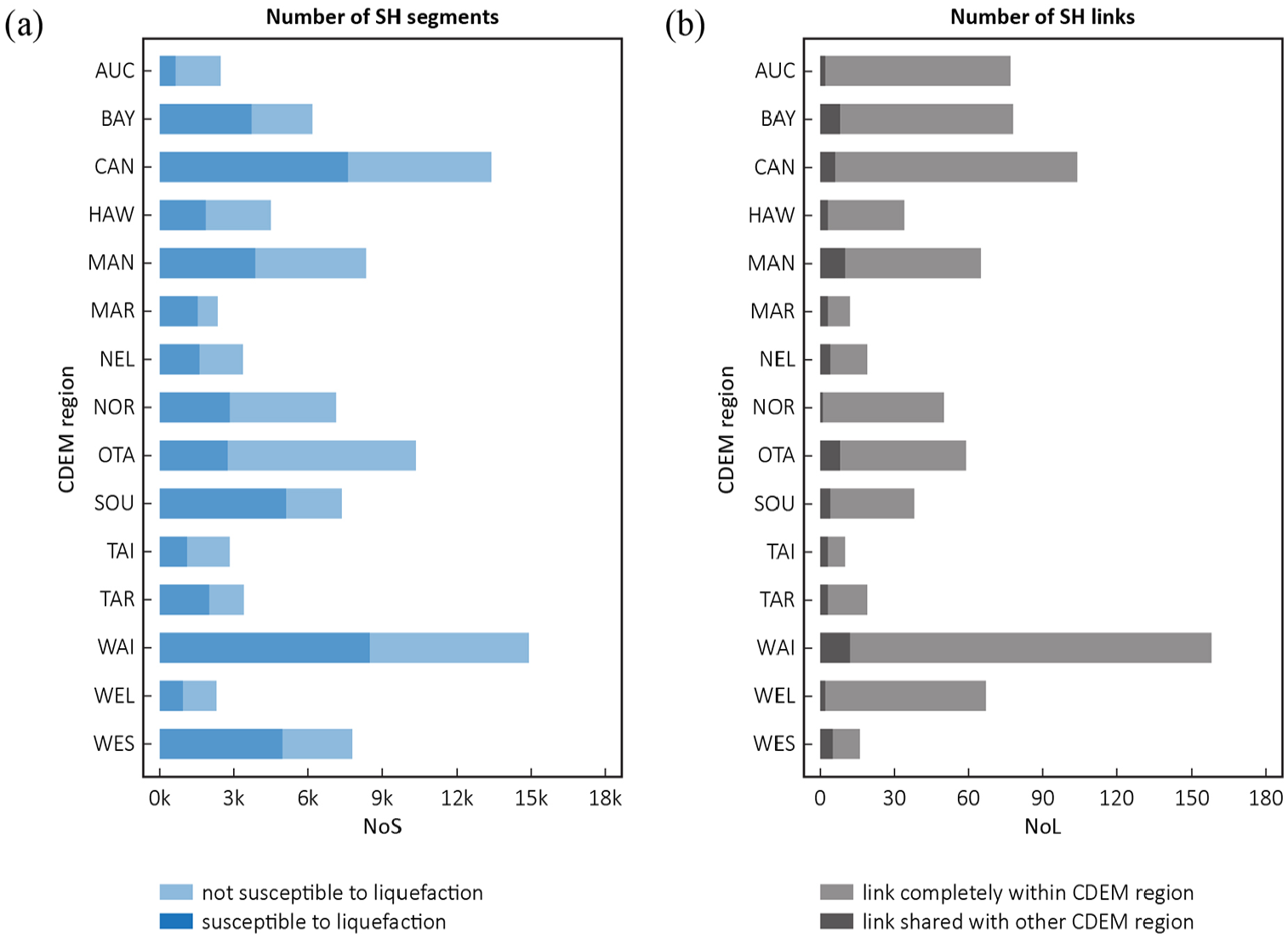
Number of State Highway (a) Segments (NoS) and (b) links (NoL) in each CDEM region (abbreviations for the regions are explained in Figure 2b). NoS presents the ratio of susceptible versus not susceptible segments, while NoL presents the ratio of links that are completely within the CDEM region versus links that are shared between two CDEM regions.

The segments between two intersections are then dissolved into links in order to better account for the interconnectivity of the network; for example, the exposure of a segment impacts the transport services along the entire link. To limit the number of links, particularly in urban areas with a dense network of local roads, only intersections with major local roads are considered. The number of links (NoL) predicted to be affected by liquefaction manifestation is calculated to further compare and evaluate liquefaction exposure across the State Highway network. Compared to NoS, which indicates the extent of potential exposure—relevant information for (national) asset management related decisions, such as infrastructure investment—NoL better accounts for the network’s interconnectivity and the potential for transport disruption across scenarios, which is particularly important for regional emergency management to ensure access to critical facilities.

As demonstrated in Figure 3b, CDEM regions with higher network densities, such as Auckland or Wellington Region, result in increased NoL. In total, the State Highway network consists of 769 links, with 37 links crossing the boundary of two CDEM regions and being considered in both regions.

For the multi-scenario assessment, the number of events (NoE) predicted to result in liquefaction manifestation in a specific segment or link is used as an additional indicator to quantify and compare exposure across CDEM regions. As a heuristic metric, NoE allows for an alternative method to evaluate and compare liquefaction exposure across the network, presenting an intermediate approach between a deterministic single-scenario and a full probabilistic hazard assessment.

Results

The State Highway network is evaluated for liquefaction exposure regarding the extent of potential exposure based on NoS, and the extent of potential service disruption based on NoL. A CDEM region is considered affected by an earthquake scenario if it contains at least one State Highway segment or link that is predicted to experience liquefaction manifestation for a specific return period or earthquake scenario. For individual scenarios, such as worst-case scenarios, the fault source is added as reference. The definition of a worst-case scenario depends on the chosen measure: Based on NoS, it presents the event (from the selected scenarios) leading to the maximum exposure across the network, while the worst-case scenario based on NoL identifies the event with the greatest potential impact on network functionality and transport services. It is important to note that other earthquake events, not included in this study, could result in even greater impacts.

Extent of potential exposure

Return period assessment

Figure 4 presents the relative number of State Highway segments (NoS_rel = NoS divided by total number of segments) predicted to be affected by liquefaction manifestation for each return period. Based on the increase rate of the NoS_rel values, CDEM regions are categorized into low, moderate or high exposure.

Figure 4.

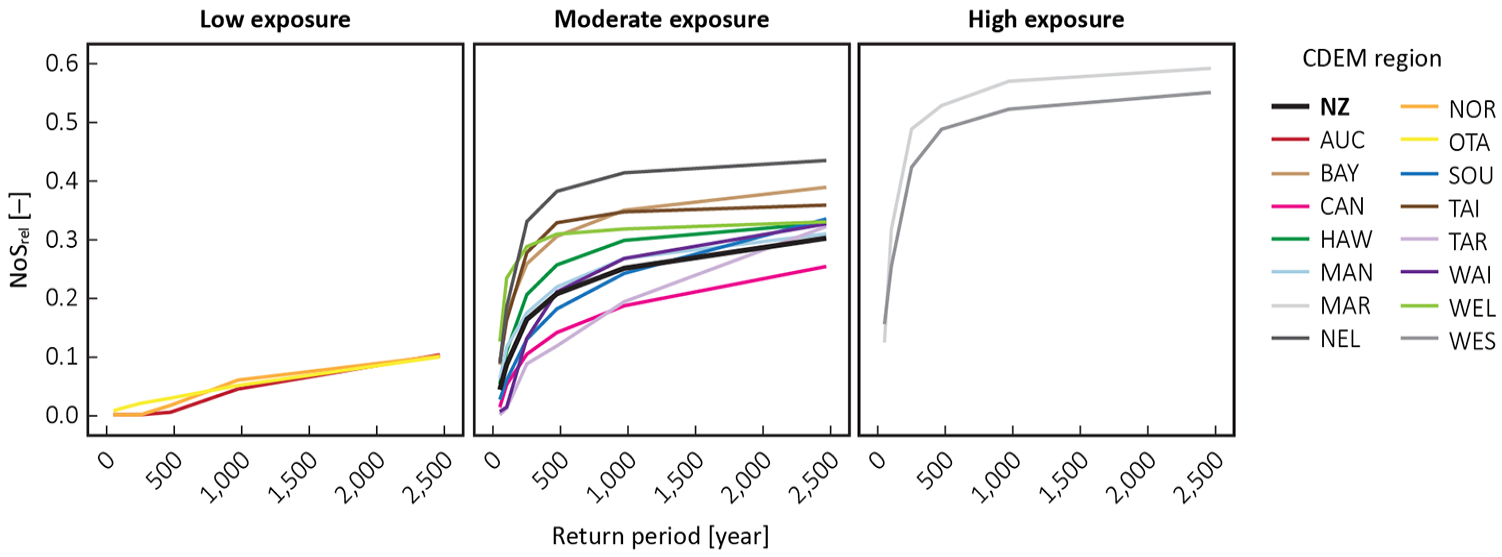
Relative number of State Highway segments (NoS_rel) predicted to experience liquefaction manifestation for different return period shaking intensities across New Zealand (NZ) as well as each CDEM region.

NoS_rel across New Zealand shows a logarithmic growth, rising rapidly for shorter return periods before the increase rate slows down for longer return periods. The results indicate that between 4.3% (50-year return period) and 30.2% (2475-year return period) of the total number of State Highway segments across New Zealand could be affected by liquefaction manifestation.

Low exposure. Auckland, Northland and Otago lead to much lower NoS_rel compared to the national results, showing values of 10.2% or below for the maximum return period. The graphs suggest a slower increase of NoS_rel between the 50-year to 975-year return periods. These regions present a relatively low percentage (30.8% on average) of susceptible segments (Figure 3a), explaining the low exposure results. In addition, Auckland and Northland are located in the northernmost area of New Zealand, which is considered seismically less active due to their distance to known fault sources.

Moderate exposure. The majority of CDEM regions show graphs with a growth pattern similar to the national results, yet, leading to slightly lower (e.g. Canterbury) or higher (e.g. Nelson Tasman) NoS_rel values. Differences can be observed for Bay of Plenty, Southland, Taranaki and Waikato, presenting a more rapid increase of NoS_rel between the 252/475-year and the 2475-year return periods. As a result, they exceed the maximum values of most CDEM regions in this category despite lower NoS_rel across shorter return periods. In addition to their proximity to the investigated fault lines (Figure 2a), these regions show a higher percentage of susceptible State Highway segments, ranging from 57.0% (Waikato) and 69.4% (Southland) (Figure 3a).

High exposure. Maximum liquefaction exposure can be observed for Marlborough (NoS_rel ≤ 59.2%) and West Coast (NoS_rel ≤ 55.1%). These CDEM regions are located on the South Island of New Zealand, which is primarily characterized by mountainous terrain. However, they also include low-lying areas, mostly consisting of alluvial plains, particularly along the coast (Barrett, 2021; Marlborough District Council, 2021). State Highways often run along or cross these susceptible areas, increasing the likelihood of the regions being affected by liquefaction manifestation during an earthquake. As illustrated in Figure 5, most State Highways in Marlborough are situated in the Wairau and Southern Valleys, which are considered highly susceptible to liquefaction. 65.5% of State Highway segments are considered susceptible to liquefaction in this region (Figure 3a). Consequently, even the lower shaking associated with a 101-year return period is estimated to result in liquefaction manifestation across 31.7% of the network (Figure 5a). For the 2475-year return period, nearly all State Highway segments in the valleys are predicted to experience liquefaction manifestation (Figure 5b). However, as return-period ground shaking represents statistically derived shaking levels rather than specific earthquake scenarios, these results do not reflect the outcome of any single event.

Figure 5.

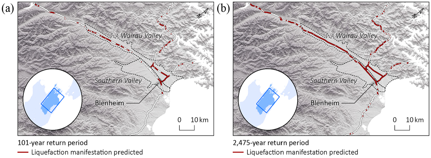
Prediction of liquefaction manifestation for State Highway segments in Marlborough based on a (a) 101-year return period shaking and (b) 2475-year return period shaking.

Multi-scenario assessment

Figure 6 presents NoS_rel for the 479 earthquake scenarios (blue lines) and for each return period (black dots). The NoE for New Zealand and each CDEM region is also summarized in Figure 6. On a national scale, 388 out the 479 earthquake scenarios are estimated to result in liquefaction manifestation in at least one State Highway segment. At the national scale, NoS_rel values across the scenarios range from 0.001% (1 segment) to 2.3% (2221 segments). Comparing these values with the results of the return periods shows that none of the scenarios exceeds the NoS_rel of any return period (where values are ≥3.0%). This highlights the differences in the scale of the exposure between a return period- and a scenario-based assessment at the national scale, given that each return period does not represent the exposure patterns and extent of single earthquake scenarios.

Figure 6.

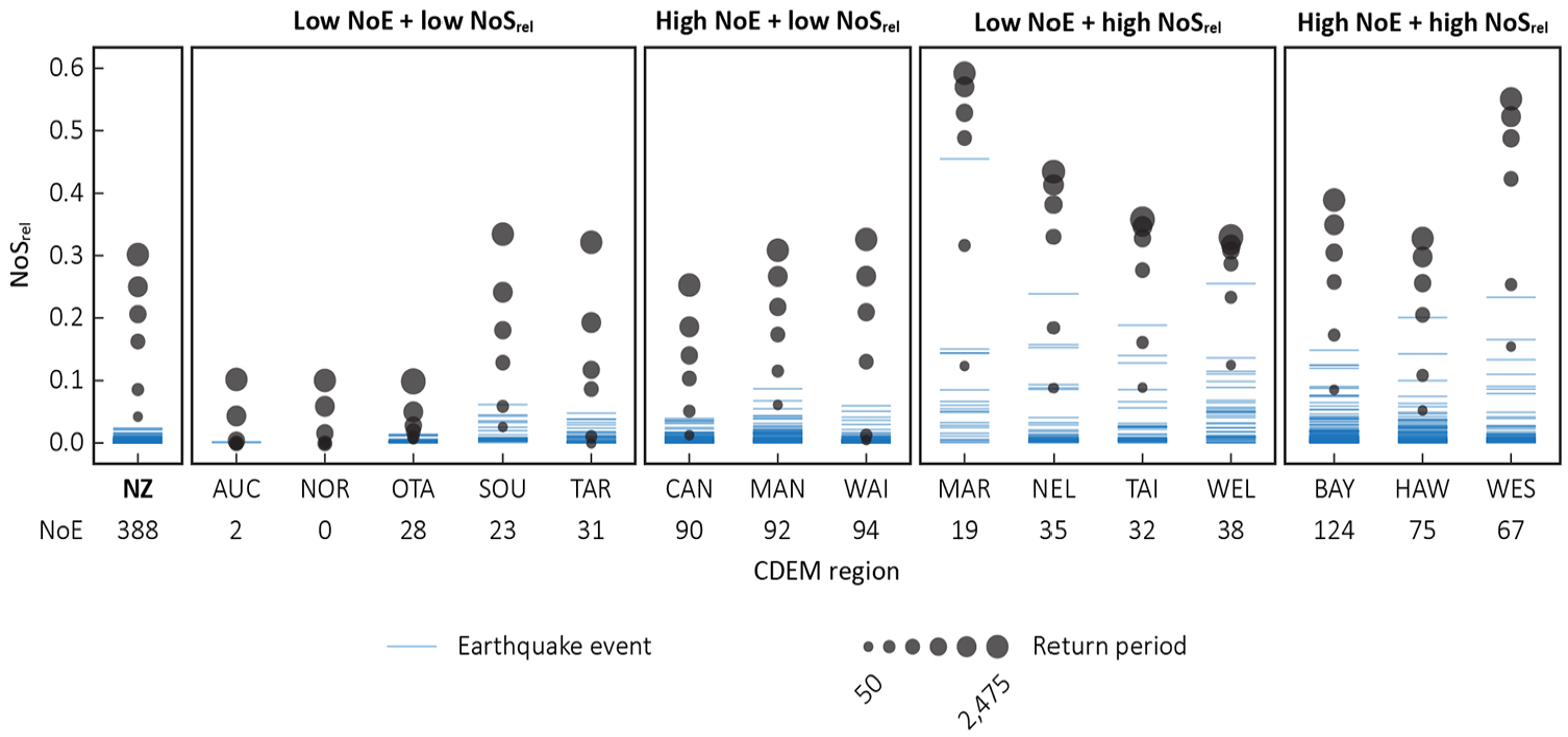
Relative number of State Highway segments (NoS_rel) and number of events (NoE) predicted to experience liquefaction manifestation for 479 earthquake scenarios across New Zealand as well as each CDEM region. NoS_rel values for the return period assessment are included for comparison.

The two scenarios with the highest NoS_rel are shaking events along the Alpine Fault in the South Island, one of the longest (approx. 850 km) and fastest moving plate boundary transform faults in the world (Berryman et al., 2012). Liquefaction manifestation caused by a M_W 8.1 rupture of the southern segment and a M_W 7.7 rupture of the northern segment are predicted to affect 2.3% and 2.1% of the State Highway network, respectively. Figure 7 presents the results of the worst-case scenario among the events assessed in this article (rupture of southern segment), highlighting that most of the predicted liquefaction manifestation occurs along the State Highway in the West Coast, connecting Wanaka and Kumara Junction. Liquefaction manifestation is also predicted along State Highways accessing Milford Sound and Mt Cook, demonstrating the large-scale impact across multiple routes in the South Island. Given the variable ground characteristics across the affected area, the implications of the manifestation would be different from one area to the next, with alluvial deposits dominated by sands in some areas and gravel in others. As mentioned previously, more site-specific assessments are needed to assess these effects in more detail.

Figure 7.

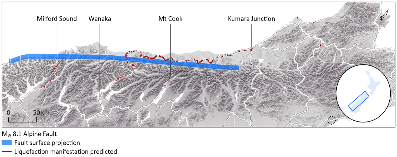
Predicted liquefaction manifestation across State Highway segments for the worst-case scenario in New Zealand. The dashed circle highlights the location of three affected segments on the east coast of the South Island.

While the NoS_rel of each event remains below the values of the return periods on a national-scale, CDEM regions present several earthquake scenarios with NoS_rel greater than the return period results, emphasizing the difference between national and regional assessments. Details of the CDEM regions are discussed in the following sections, which categorize each region according to their NoS_rel and NoE results:

• Low NoE + low NoS_rel: Results suggest low exposure to liquefaction manifestation due to limited number of earthquakes affecting the CDEM region and low number of State Highway segments potentially exposed.

• High NoE + low NoS_rel: Although potential exposure is expected to be limited, high NoE indicates that the State Highway network could be affected more frequently. Repeated impacts may drive stakeholders to invest in prevention measures in order to reduce economic loss.

• Low NoE + high NoS_rel: Liquefaction manifestation is predicted to affect a larger extent of State Highways. Emergency management may prioritize a specific event (e.g. worst-case scenario) over others for planning purposes as it could significantly impact the network. Because of the relatively low NoE, the consequences of repeated exposure are less relevant in this case.

• High NoE + high NoS_rel: High exposure to liquefaction manifestation, implying frequent and potentially extensive impact across State Highways. Specific network sections and/or specific scenarios should be further investigated in order to prioritize mitigation efforts and to prepare for emergency situations.

It should be noted that the NoE in Figure 6 refers to the number of events affecting the CDEM region (max NoE = 124), while the NoE in the maps present the number of events affecting an individual State Highway segment (max NoE = 39).

Low NoE + low NoS_rel. Low liquefaction exposure is estimated for Auckland, Northland, Otago, Southland and Taranaki, presenting low NoE (≤ 31) and NoS_rel (≤ 6.1%). Northland is the only CDEM region that is not affected by any of the 479 events (NoE = 0). While the return period assessment indicates low exposure for Otago (Figure 4), the findings of the multi-scenario evaluation suggest a slightly higher potential exposure in this region due to NoS_rel values up to 1.3% and a NoE of 28.

Based on the return period results, Southland and Taranaki are categorized as moderately exposed (Figure 4), whereas the multi-scenario approach implies lower exposure compared to other CDEM regions.

High NoE + low NoS_rel. CDEM regions with high NoE (≥90) and low NoS_rel (≤8.6%) include Waikato, Manawatū-Whanganui and Canterbury. The high NoE can be partly explained by the large size of the regions as the maximum NoE of an individual State Highway segment only ranges between 15 (Waikato) and 27 (Manawatū-Whanganui). Furthermore, increased NoE is limited to specific locations within the CDEM region, with the majority of segments (up to 84%) presenting a NoE of 0, indicating no exposure for any earthquake scenario. In Manawatū-Whanganui, State Highways in the southern part show elevated NoE values up to 27 (Figure 8a).

Figure 8.

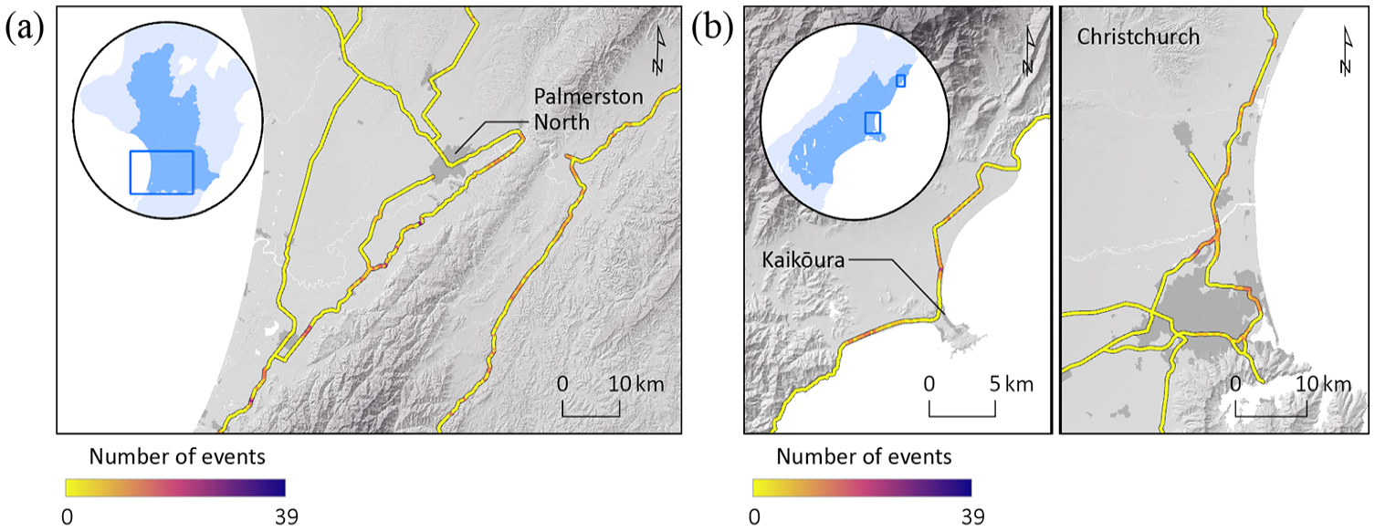
Number of events across State Highway segments in (a) Manawatū-Whanganui and (b) Canterbury.

State Highway segments with increased NoE in Canterbury are mainly situated near Kaikōura (NoE ≤ 20) and Christchurch (NoE ≤ 16) (Figure 8b). Both areas are considered highly susceptible to liquefaction, which became evident during the 2010–2011 Canterbury Earthquake Sequence (Cubrinovski et al., 2014) and the 2016 Kaikōura earthquake (Kaiser et al., 2017).

Low NoE + high NoS_rel. Despite a relatively low NoE of 19, Marlborough presents the event with the highest NoS_rel: A M_W 7.8 earthquake along the Wairau Fault is estimated to result in liquefaction manifestation across 45.8% of the State Highways in this region. Compared to the NoS_rel distribution of other CDEM regions, the worst-case scenario of Marlborough significantly exceeds the NoS_rel of the remaining 18 events (Figure 6). As demonstrated in Figure 9a, the Wairau Fault is largely parallel to or intersects the network, explaining the spatial extent of liquefaction manifestation estimated for this scenario.

Figure 9.

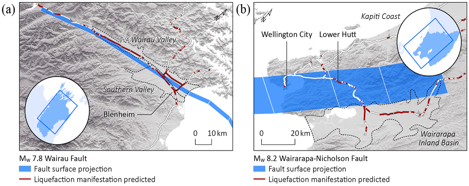
Predicted liquefaction manifestation across State Highway segments for the worst-case scenario in (a) Marlborough and (b) Wellington Region.

Another example of a CDEM region with low NoE and a distinctive worst-case scenario is Wellington Region (Figure 9b). The M_W 8.2 rupture of the Wairarapa-Nicholson Fault results in a much higher NoS_rel of 25.5% than the remaining 37 events (NoS_rel ≤ 13.6%). The worst-case scenario primarily affects State Highways in the Wairarapa Inland Basin and Lower Hutt, which are considered highly susceptible (Hancox, 2005).

The findings of Marlborough and Wellington Region suggest that emergency management may prioritize these scenarios for planning as it results in significantly higher liquefaction exposure compared to other events.

High NoE + high NoS_rel. Bay of Plenty presents the highest NoE based on CDEM regions (124) as well as individual State Highway segments (39). As illustrated in Figure 10a, segments in Edgecumbe and Whakatāne have the maximum NoE values. This area is exposed to numerous faults (Figure 2a) and is considered highly susceptible to liquefaction because of its low elevation (shallow water table depth) and alluvial deposits (Bastin et al., 2020). Liquefaction manifestation was observed in this area in the 1987 Edgecumbe earthquake (Bastin et al., 2020).

Figure 10.

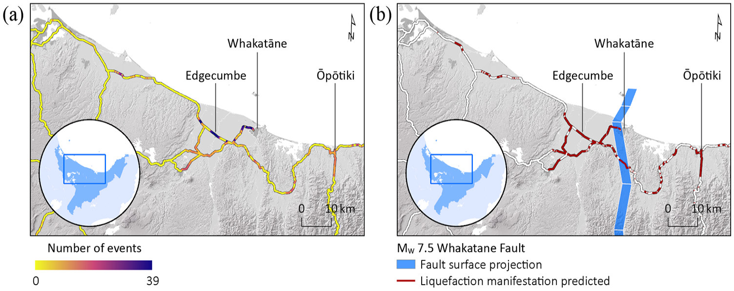
(a) Number of events across State Highway segments in Bay of Plenty. (b) Predicted liquefaction manifestation for the worst-case scenario.

In addition to increased NoE, Bay of Plenty presents comparatively high NoS_rel values up to 14.8%. However, 60% of the events are predicted to result in liquefaction manifestation in less than 1.0% of State Highways. The worst-case scenario is a M_W 7.5 rupture of the Whakatāne Fault, which is expected to result in extensive liquefaction manifestation along several State Highways providing access to Edgecumbe, Whakatāne and Ōpōtiki (Figure 10b).

Due to increased NoE as well as NoS_rel, State Highways in Bay of Plenty can be categorized highly exposed to liquefaction manifestation. Hawke’s Bay and West Coast also fall under this category, showing NoE up to 75 and 67, respectively, and NoS_rel up to 20.0% and 23.3%, respectively (Figure 6).

Extent of potential service disruption

Return period assessment

Figure 11a presents the minimum return period expected to result in liquefaction manifestation across State Highway segments, emphasizing that a large portion of the network (69.8%) has no liquefaction manifestation predicted for any return period. Converting segments to links by identifying the maximum liquefaction probability between two intersections (Figure 11b) reduces the percentage of network that is expected to remain unaffected (28.9%). Furthermore, while only 4.3% of segments indicate higher exposure as they are estimated to experience liquefaction manifestation for the shortest return period (50-year), 17.6% of State Highway links are assigned to this category, demonstrating the potential impact of using individual segments to characterize the impact on the wider network.

Figure 11.

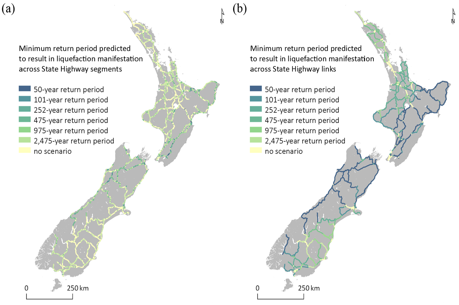
Minimum return period predicted to result in liquefaction manifestation based on State Highway (a) segments and (b) links.

To further examine the difference between the evaluation of NoS_rel versus the relative number of State Highway links (NoL_rel = NoL divided by total number of links) predicted to be affected by liquefaction manifestation, both indicators are compared for each return period in Figure 12. CDEM regions are categorized based on their increase in NoL_rel, reflecting changes in exposure when evaluating State Highway links instead of segments.

Figure 12.

Relative number of State Highway links (NoL_rel) predicted to experience liquefaction manifestation in relation to NoS_rel for different return periods across New Zealand as well as each CDEM region.

No or slow increase. Marlborough, Tairāwhiti and West Coast present very slow increase in NoL_rel across the return periods, that while the number of affected segments may rise, the overall number of affected links remains relatively constant. For the West Coast, NoL_rel values show no increase, remaining at 93.8% across all return periods. In these three CDEM regions, NoL_rel values are consistently high (up to 100% in Marlborough), even at shorter return periods. This likely reflects the smaller number of total links (approx. 14 on average, Figure 3b) but greater length per link (approx. 39 km on average), suggesting a higher likelihood of affected segments within each link across any return period.

Wellington Region also presents a slow increase in NoL_rel; however, with lower values compared to other regions in this category, showing that between 29.9% (50-year return period) and 55.2% (2475-year return period) of the network links could be disrupted. As illustrated in the hazard maps (Figure 13), the 2475-year return period only presents a slightly higher number of affected links, primarily across Wellington City and Kapiti Coast (Figure 13b), compared to the 252-year return period (Figure 13a).

Figure 13.

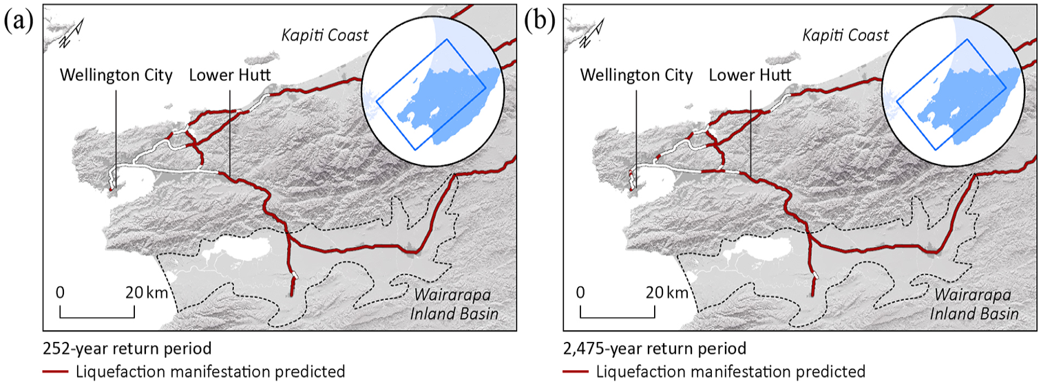
Predicted liquefaction manifestation for State Highway links in Wellington Region based on a (a) 50-year return period and (b) 2475-year return period shaking.

Moderate increase. The NoL_rel of the entire network (New Zealand) and most CDEM regions show moderate increase, with NoL_rel values rising by an average of 44.6% points between the 50- and 2475-year return periods. Unlike the CDEM regions of the previous category (no or slow increase), the level of network disruption is more clearly influenced by the return period in these CDEM regions.

Rapid increase. Rapid increase can be observed for Bay of Plenty, Northland, Southland, Taranaki and Waikato. Waikato presents the largest increase of NoL_rel (+ 50.0% points) between two return periods, indicating that the percentage of affected links could rise from 10.1% (101-year return period, Figure 14a) to 60.1% (252-year return period, Figure 14b). Although seismic hazard is considered low compared to other CDEM regions, Waikato may experience liquefaction manifestation across the Hauraki Plain or Hamilton Basin (Dredge, 2014; Villamor et al., 2024). Most State Highway links (75.3%) cross these susceptible areas, leading to high NoL_rel up to 83.5% despite NoS_rel values not exceeding 32.6% for all return periods.

Figure 14.

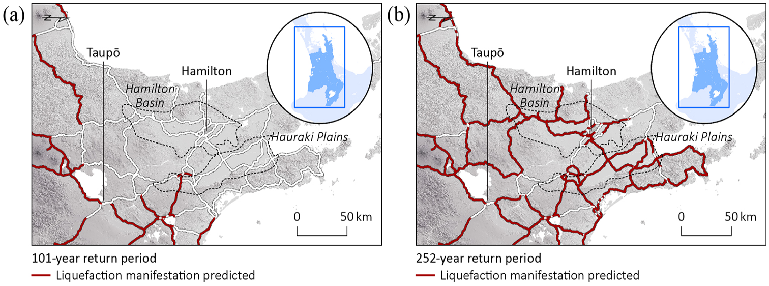
Predicted liquefaction manifestation for State Highway links in Waikato based on a (a) 101-year return period and (b) 252-year return period shaking.

Multi-scenario assessment

Figure 15 compares NoE based on State Highway segments and links. Similar to the return period assessment (Figure 11), the NoE map for the segments highlights that most of the network (78.4%) presents no exposure to liquefaction manifestation during any of the 479 earthquake scenarios (Figure 15a), while estimation based on links indicates that only 44.9% of the network remains unaffected (Figure 15b). The increase of the maximum NoE from 39 to 59 when evaluating State Highway links further emphasizes the role of spatial context for the exposure assessment as high values are primarily observed for longer links, such as State Highway 35 or 6, which are more likely to be affected during an earthquake given their positions closer to plate boundaries and larger numbers of active faults.

Figure 15.

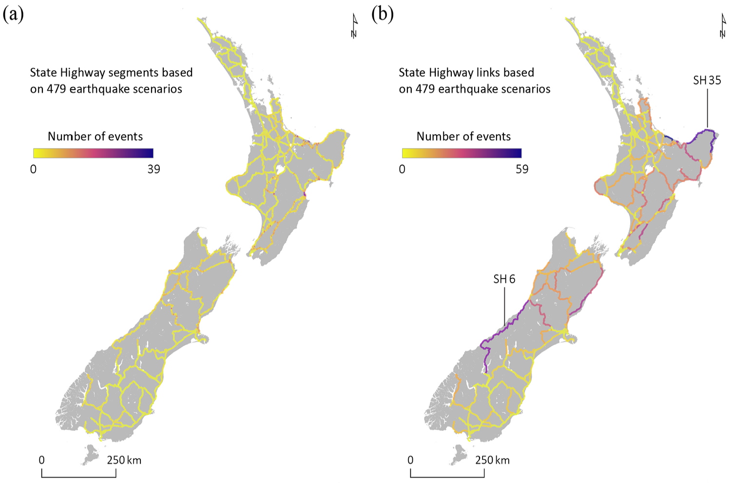
Number of events across State Highway affecting (a) segments and (b) links.

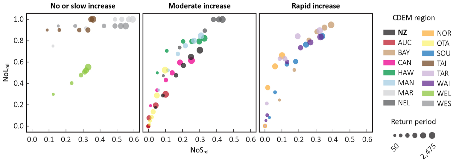
Figure 16 presents the relationship between NoS_rel and NoL_rel for each earthquake scenario and each CDEM region. The figure does not include Northland as none of the investigated events affect the State Highway network. Apart from Auckland (Figure 16b), all CDEM regions show an increase in NoE when assessing State Highways based on links, suggesting that transport services in most regions could be affected by liquefaction manifestation occurring in a different region. The distribution of NoE across the groups based on links aligns with the distribution of NoE based on segments. For example, Bay of Plenty presents the highest NoE, suggesting that 137 events could affect links associated with this region (Figure 16c). However, a few CDEM regions show a more significant increase in NoE. For example, Tairāwhiti may be impacted by 45 additional events when assessing liquefaction hazards based on links (Figure 16k). Three out of 10 links in this region cross the boundaries with Bay of Plenty and Hawke’s Bay. Those links are relatively long (e.g. State Highway 35, Figure 15b), increasing the likelihood of containing State Highway segments that are exposed to liquefaction manifestation outside of Tairāwhiti. A similar situation is observed for Otago (Figure 16i), presenting an increase in NoE of 27 due to a shared link crossing into the West Coast (State Highway 6, Figure 15b).

Figure 16.

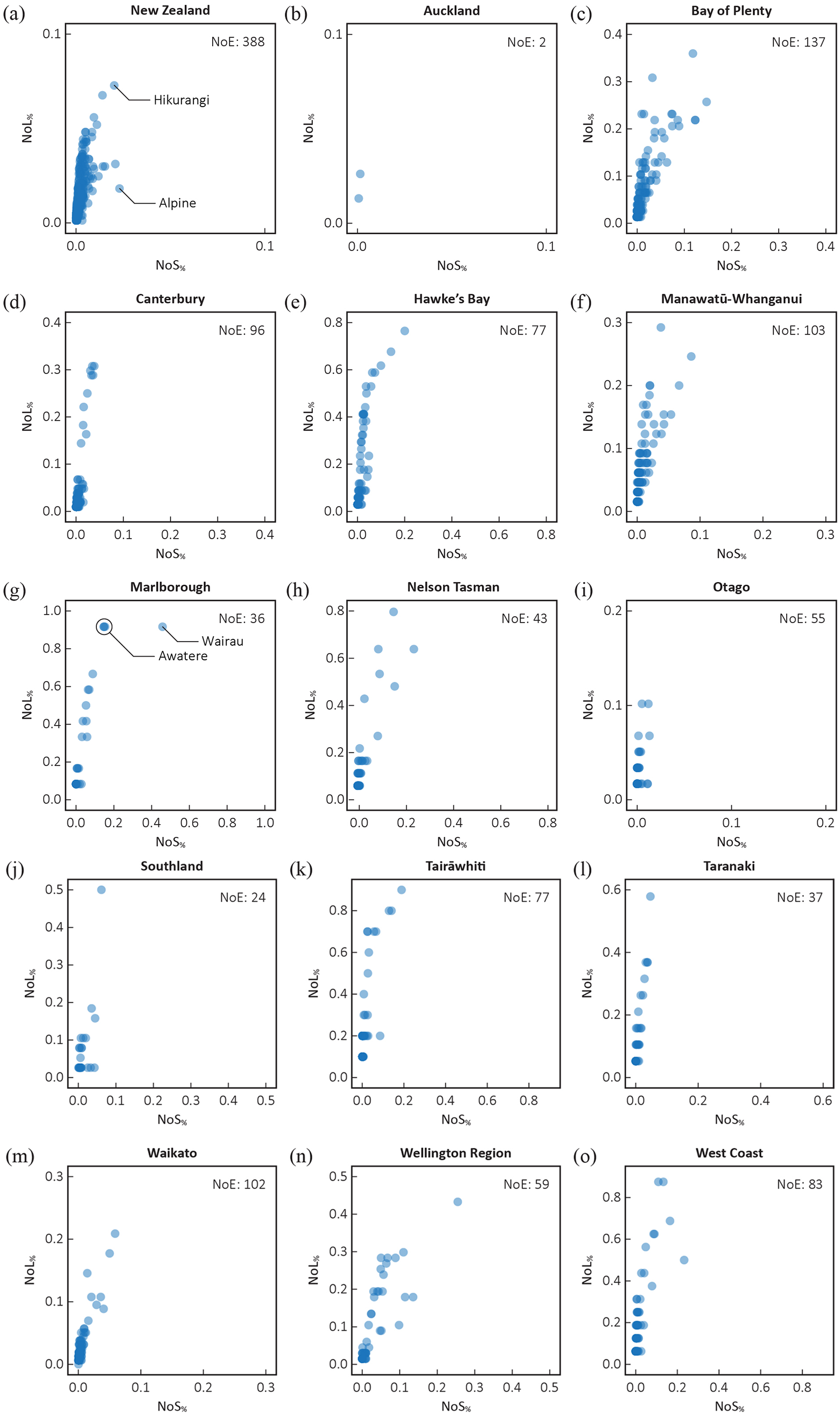
Relative number of State Highway links (NoL_rel) predicted to experience liquefaction manifestation in relation to NoS_rel for 479 earthquake scenarios, including the number of events (NoE): (a) New Zealand, (b) Auckland, (c) Bay of Plenty, (d) Canterbury, (e) Hawke’s Bay, (f) Manawatū-Whanganui, (g) Marlborough, (h) Nelson Tasman, (i) Otago, (j) Southland, (k) Tairāwhiti, (l) Taranaki, (m) Waikato, (n) Wellington Region and (o) West Coast.

Further details on the relationship of NoS_rel and NoL_rel are provided in the following sections, classifying CDEM regions according to common characteristics.

Variation across low NoS_rel-events. Similar to the findings of the return period assessment, most CDEM regions show a significant increase of NoL_rel compared to NoS_rel when evaluating the 479 earthquake scenarios. Some regions indicate that events may lead to similar numbers of affected segments but result in different numbers of affected links. For example, most scenarios that estimated liquefaction manifestation across segments in Hawke’s Bay lead to a NoS_rel of less than 3%, implying consistently low exposure. However, NoL_rel varies across these events, ranging from 2.9% to 41.2% (Figure 16e). This suggests that NoL_rel could be used for CDEM regions with large numbers of low NoS_rel events, allowing for a better distinction and possibly prioritization of earthquake scenarios. Similar findings can be observed for Manawatū-Whanganui (Figure 16f), Tairāwhiti (Figure 16k) and West Coast (Figure 16o).

Amplification of worst-case scenario. The worst-case scenarios of Southland (Figure 16j) and Taranaki (Figure 16k) demonstrate much higher NoL_rel values, exceeding the remaining events by 31.6% points and 21.1% points, respectively. As illustrated in Figure 17, segments predicted to be exposed to liquefaction manifestation during the M_W 7.5 shaking of the Hokonui Fault are distributed across the network in Southland (Figure 17a), impacting 19 out of 38 links (Figure 17b). This event could disrupt access to Invercargill, the most populated city in this region, as well as Milford Sound and Te Anau, which are important tourist destinations.

Figure 17.

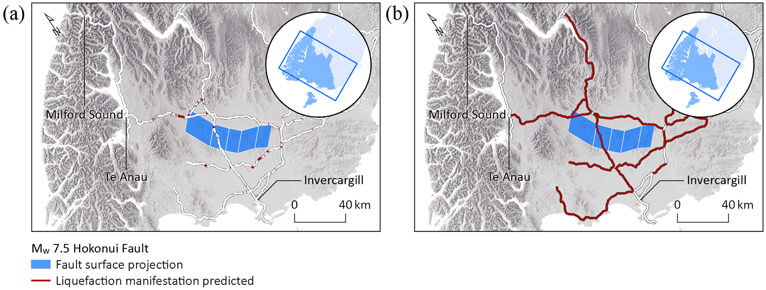
Liquefaction manifestation predicted for the Southland worst-case scenario across State Highway (a) segments and (b) links.

Change in worst-case scenario. Half of the CDEM regions present different worst-case scenarios between NoS_rel and NoL_rel, which could change the outcome of the exposure assessment and affect decision-making. This includes the worst-case scenario based on the national-scale prediction. A M_W 8.4 shaking of the Hikurangi Subduction Zone results in the maximum NoL_rel, estimated to affect 7.3% of the State Highway links (Figure 16a). This event affects segments along the entire east coast of the North Island (Figure 18a), which could lead to large-scale disruptions, involving multiple CDEM regions and potentially affecting access to Napier, Wairoa, Gisborne, Ōpōtiki and Whakatāne (Figure 18b).

Figure 18.

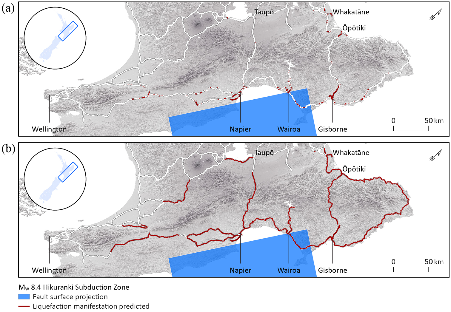
Liquefaction manifestation predicted for a rupture of the Hikurangi Subduction Zone across State Highway segments and (b) links.

The M_W 8.1 Alpine Fault scenario, which is considered the worst-case scenario for New Zealand State Highways based on NoS_rel, only presents a NoL_rel of 6.2%. This value is below the NoL_rel of several other events with much lower NoS_rel (Figure 16o). Despite indicating the most extensive exposure, the majority of affected segments (97.7%) belong to the same State Highway link connecting Wanaka and Kumara Junction (Figure 7). Therefore, consequences for the wider network may be less significant compared to other earthquake scenarios.

Marlborough presents the CDEM region with the highest NoL_rel with values up to 91.7%. Maximum NoL_rel is achieved for 4 scenarios, including the M_W 7.8 Wairau event, the worst-case scenario based on State Highway segments, and three M_W 7.6/M_W 7.7 events related to the Awatere fault (Figure 16 g). Due to the distribution of the Marlborough network, most links cross alluvial plains, increasing the likelihood of experiencing liquefaction manifestation during earthquakes. This example illustrates that several events can lead to similar or higher disruptions in transport services despite involving fewer segments exposed to liquefaction manifestation.

Discussion

Using the New Zealand State Highway network as a case study, this study explores different approaches for assessing liquefaction exposure across road networks in order to inform different aspects of asset management and emergency planning. The following sections summarize the findings and discuss limitations and uncertainties as well as potential areas for future research.

Return period versus earthquake scenarios

A key result of this study is the comparison of return periods and individual earthquake scenarios for predicting liquefaction exposure across large-scale infrastructure, highlighting their respective advantages and limitations. The return period method provides a recurrence-based framework, estimating exposure likelihood over defined timeframes, which can be particularly useful for long-term asset management, allowing for the prioritization of investments in regions with the highest expected exposure. However, estimates generally show higher exposure (NoS_rel and NoL_rel values) and may present very different results compared to the multi-scenario approach. Examples, such as Northland, demonstrate how the selection of the ground shaking input can impact the assessment and potentially influence decision-making. In this region, no active faults have been identified to inform the NSHM, and instead the hazard is representative of the methods used to represent the background seismicity.

Furthermore, the evaluation of the return period analysis only focuses on NoS_rel and NoL_rel, while the multi-scenario assessment provides an additional indicator (NoE) to compare estimates across regions: The number of events adds a new dimension to the analysis by investigating which network segments and links could be repeatedly affected by liquefaction manifestation across multiple events. The findings show that the use of NoE results in a different exposure classification when comparing regions (e.g. Marlborough and Hawke’s Bay). Again, this illustrates the impact of each approach on the outcome of the analysis and, ultimately, on decision-making.

The results highlight significant differences in estimated liquefaction exposure across the network between the return period-based and multi-scenario assessments. While this article aims to demonstrate and explore those differences, it is important to emphasize that the two approaches serve different purposes and are typically applied at different scales. Return period assessments are often conducted at a smaller scale and are particularly useful for stakeholders involved in asset-specific engineering design and assessment. Multi-scenario assessments, or even evaluations based on a single scenario, however, are more appropriate for larger-scale planning, such as network operation or emergency management planning, focusing on understanding the spatial extent and consequence of disruptions.

It is also important to highlight the limitations in this study that can be addressed in future research. Despite covering a wide range of potential scenarios, 479 events only account for a small portion of possible fault ruptures in New Zealand. Future research should include more scenarios to achieve a more robust evaluation and to further explore NoE as an indicator for liquefaction exposure. This includes the representation of different magnitude events on single-fault sources, as smaller magnitudes than those considered here could still result in liquefaction manifestation. Additional scenarios should also involve the rupture of multiple faults (e.g. 2016 Kaikōura earthquake) as they could affect larger parts of the network compared to single-fault ruptures and provide a more accurate representation of distributed seismicity in the context of network assessment.

Incorporating additional fault ruptures may include the occurrence rates of each scenario, allowing for a more probabilistic representation of the liquefaction exposure. This could shift the output of the evaluation toward events that are more likely to occur and provide further information for decision-making. Although a likelihood-weighted assessment may be less useful for emergency management planning, as the results provide more room for interpretation and may not translate directly into operational actions, it may benefit network owners or operators interested in risk-based analysis to support decision-making regarding long-term asset planning, or performance-based investment strategies.

Furthermore, future research could explore a more comprehensive analysis based on the return period shaking by performing a full probabilistic liquefaction hazard analysis (PLHA), where the liquefaction probability at each shaking level is linked to the corresponding annual exceedance rates of ground shaking. Consistent with performance-based earthquake engineering, this would allow for the estimation of annualized liquefaction rates or the probability of liquefaction manifestation over a defined time frame. Provided that reliable estimates for liquefaction probability or severity are available, a PLHA could improve comparability across locations and support decision-makers focusing on liquefaction risk.

Future research could also apply both the return period and multi-scenario approaches to other co-seismic hazards, such as landslides, which may expose roads located in mountainous terrain during earthquakes. Expanding the scope to capture all seismic and co-seismic hazards allows for a more robust framework for predicting network disruptions, and provides further insight into the application of the two approaches to different aspects of decision-making.

National- versus regional-scale assessments

National-scale assessments offer a broad overview of liquefaction exposure, useful for strategic planning and resource allocation across entire networks. However, the findings demonstrate the value of regional-scale assessments, particularly for the multi-scenario approach. The evaluation at a CDEM level demonstrates high variability across sets of events and provides valuable information, including the identification of worst-case scenarios for specific regions. The spatial distribution of predicted liquefaction manifestation or NoE suggests that further downscaling may be necessary for (large) CDEM regions characterized by contrasting landforms (e.g. mountains and plains), such as Manawatū-Whanganui and Canterbury. In these cases, increased liquefaction exposure is limited to specific State Highway segments or links and may not be well reflected in quantitative measures, such as NoS_rel or NoL_rel, which are calculated for the network of the entire region.

State Highway segments versus links

The conversion of State Highway segments into links provides a clearer picture of the wider impact of liquefaction manifestation on transport services. The representation of interconnectivity could further benefit from incorporating other network characteristics, such as network redundancy. More populated areas with higher NoL likely present higher connectivity, which may indicate the presence of redundant/alternative routes, potentially reducing the overall network vulnerability. Future research could further investigate the role of network redundancies in mitigating the functional impact of liquefaction exposure, particularly in urban areas where network density (NoL) is higher.

In this context, future research could also explore network criticality, particularly for return period and scenario assessments that affect a large number of State Highway links, as it helps prioritize State Highways that are more important for both business-as-usual and post-event road functions. Relevant data for quantifying criticality could include traffic volume and freight value, both of which influence the economic and social impact of network disruptions.

It is important to acknowledge the sensitivity of the chosen segment length, as this introduces uncertainty in the results. The segment length is primarily determined by the resolution of the liquefaction model inputs and output; thus, different resolutions may lead to variations in NoS values. A finer resolution, allowing for shorter segments, may capture more localized variations in liquefaction susceptibility, potentially increasing the number of affected segments, while coarser resolutions leading to longer segments may smooth out localized effects, reducing NoS. This is particularly relevant for applications outside New Zealand, where large-scale liquefaction models may have lower spatial resolution, requiring adjustments of the segment length to maintain consistency. In regions where higher-resolution models are available, shorter segment lengths could improve spatial accuracy. Future research should explore the sensitivity of NoS to segment length across different model resolutions to better understand potential impacts on the assessment.

Other limitations

An important limitation arises from the geospatial model used to calculate the liquefaction probability for the return periods and the earthquake scenarios. Due to the lack of subsurface data, the model is unable to account for detailed site-specific soil characteristics and geomorphic effects, which are relevant for liquefaction triggering and propagation (Russell and Van Ballegooy, 2015; Zhu et al., 2015). In addition, the estimated WTD introduces uncertainty, particularly due to seasonal fluctuations in groundwater levels. As observed during the 2010–2011 Canterbury Earthquake Sequence, differences in the water table depth contributed to variations in liquefaction extent and severity between the June and December events, despite similar ground shaking patterns (Russell and Van Ballegooy, 2015). Furthermore, research on the liquefaction manifestation observed during the 2016 Kaikōura earthquake indicates that the New Zealand specific model tends to overestimate liquefaction hazards along water bodies and presents uncertainties across regions with rapidly changing elevations, such as mountains, as it causes fluctuations in the variables Vs30 and WTD (Lin et al., 2022), potentially leading to underestimation.

Another aspect to consider when evaluating liquefaction hazards across infrastructure networks is the model’s inability to predict liquefaction manifestation type and severity, which is essential for estimating the potential damage to the road network. For example, liquefaction-induced lateral spreading is more likely to result in extensive damage to the road, significantly impacting transport services and requiring more resources and time for the recovery. Limited surface ejecta, however, may not cause structural damage, allowing for network services to continue without any restrictions or with only small reductions in road function (e.g. reduced vehicle speeds). It is important to further investigate potential impacts; for example, by incorporating geotechnical data along State Highway sections where high liquefaction exposure is predicted by the geospatial model. In this way, it can serve as a screening approach to inform this more site-specific investigation and assessment. Improvements in liquefaction estimation methods for large spatial extents would allow for a shift from binary classification to a more nuanced representation of liquefaction hazards, and would increase confidence in using these estimates in combination with return period shaking or earthquake scenarios.

Another limitation relates to the conversion from SA[0.5 s] to PGV, as the relationship is subject to variability across different site conditions and ground motion characteristics (Bommer and Alarcon, 2006). This study does not explicitly account for this uncertainty, which may affect the estimated PGV values. Since this conversion was only applied to return-period calculations, while earthquake scenarios directly use PGV values from CyberShake, there may be bias in the evaluation of the results.

Conclusions

This article provides a comprehensive evaluation of different approaches to assess liquefaction exposure across infrastructure networks, aiming to inform decision-making processes regarding asset management as well as emergency preparation and response planning. Based on the New Zealand State Highway network, different return period shaking scenarios as well as a range of individual earthquake scenarios are used to estimate the extent of potential exposure (NoS) and the level of network disruption (NoL). The findings highlight the advantages of the multi-scenario approach as it offers an additional indicator (NoE) to analyze and compare liquefaction exposure. While the national-scale assessment helps to quantify liquefaction exposure across the entire network, providing valuable insight for asset management, the regional-scale assessments identify events of particular interest, such as worst-case scenarios, and allow for more informed decision-making regarding emergency management.

Future research should address limitations associated with the underlying liquefaction model and incorporate additional events, including multi-fault ruptures, to improve the robustness of the multi-scenario approach. This includes the potential to integrate recurrence intervals to weight suites of scenarios or to expand the analysis into a full probabilistic liquefaction hazard analysis, provided that reliable liquefaction estimates, including the associate network component damage, are available. This could offer a more comprehensive representation of network exposure and risk, and provide additional support for decision-making.

Liquefaction model data

Aside from PRECIP, which is retrieved from the global weather and climate database WorldClim (Hijmans et al., 2005), all input variables for the geospatial liquefaction model are based on New Zealand specific datasets. Vs30 is estimated by Foster et al. (2019) and relies on geology- and terrain-based data as well as different sources of direct Vs₃₀ measurements across New Zealand. DW is defined as the minimum distance to the nearest coastline (LINZ, 2012), lake (LINZ, 2022a) or river of stream order 4 or higher (LINZ, 2022b). WTD is calculate by Westerhoff et al. (2018) using a New Zealand specific terrain model and long-term time series of recharge estimates.