Sage Journals: Discover world-class research

Abstract

This article develops a framework for and explores the use of case-based reasoning (CBR) to predict seismically induced liquefaction manifestation. CBR is an artificial intelligence process that solves new problems using the known answers to similar past problems. CBR sorts a database of case histories based on their similarity to a design case and predicts the outcome of the design case as the observed outcome of the most similar case history or majority outcome of the most similar case histories. Two databases of liquefaction case histories are used to develop and validate numerous CBR models. Different input parameters and aspects of the CBR method and their influence on the predictive capability of the models are evaluated. Some of the developed CBR models were shown to have a better predictive power than currently existing models. However, more research is needed to refine these models before they can be used in practice. Nevertheless, this study shows the potential of CBR as a method to estimate liquefaction manifestation and suggests several avenues of future research.

Keywords

Liquefaction artificial intelligence machine learning case-based reasoning liquefaction manifestation liquefaction demand parameters

Introduction

The most widely used methods to evaluate liquefaction triggering are based on the simplified stress-based procedure developed by Seed and Idriss (1971). This method compares the cyclic stress induced in a soil layer by an earthquake with the cyclic strength of the soil to provide a factor of safety against liquefaction. Numerous liquefaction-triggering models have been developed based on this procedure using laboratory test, cone penetration test (CPT), standard penetration test (SPT), or shear wave velocity (V_s) data to model the soil resistance. However, Cubrinovski et al. (2019) showed that these models do not accurately account for system effects, which refer to the dynamic (seismic wave propagation) and pore pressure (water flow) interaction between layers. This led to both the overestimation and underestimation of liquefaction hazard at numerous sites during the Canterbury earthquake sequence in New Zealand. In addition, liquefaction-triggering models are often used in conjunction with susceptibly models (e.g. Bray and Sancio, 2006) to evaluate whether the soil can liquefy, and liquefaction manifestation models that predict liquefaction severity (e.g. Iwasaki et al., 1978), ground settlement (e.g. Ishihara and Yoshimine, 1992), or lateral spreading (e.g. Zhang et al., 2004). However, liquefaction susceptibility, triggering, and manifestation models developed by various authors and separate datasets are often used together, and the collective uncertainty and accuracy of these different combinations is unknown. Finally, Geyin et al. (2020) found that simplified stress-based liquefaction-triggering models developed since 1998 show little improvement in their predictive capabilities, despite a significant increase in case history data. Geyin et al. (2020) suggested that real demonstrable improvement would only occur with “disruptive innovation” to the in situ test method or modeling approach. Because many manifestation models are explicitly linked to triggering models through their predicted factor of safety, this applies to manifestation models as well. Therefore, this article evaluates the use of case-based reasoning (CBR) to estimate liquefaction manifestation. This is an innovative and intuitive technique that has rarely been explored in geotechnical engineering, and similar to geospatial models that predict liquefaction manifestation, CBR models inherently merge liquefaction susceptibly, triggering, and manifestation. As a result, accuracy is clearly defined for the entire liquefaction analysis.

CBR is an artificial intelligence process in which new problems are solved using the known solutions to old problems (Aamodt and Plaza, 1994). A new problem, or design case, is compared to a database of old problems, or case histories, and the outcome of the case history that is the most similar to the design case (or majority outcome of the most similar case histories) is used to predict the result of the design case. In essence, CBR is reasoning by analogy or association based on the experience from previous similar cases. This is a technique that people use all the time in their everyday lives. For example, lawyers use it to justify arguments in new cases, and doctors and car mechanics can use it to quickly diagnose problems and suggest solutions (Kolodner, 1992). CBR is particularly useful in domains where there is incomplete information, which is often the case in geotechnical engineering where subsurface data are limited. This is even more true for regional geotechnical analyses. Therefore, CBR could be beneficial for liquefaction hazard evaluations at the site and regional level.

The CBR method is not a new technique, but it has only been applied to geotechnical engineering purposes for very limited proof-of-concept studies (e.g. Engin et al., 2018; Roberts and Engin, 2019). To date, the majority of CBR applications in civil engineering have been in the construction management field where it is used to estimate project cost (Kim and Shim, 2014; Lesniak and Zima, 2018), construction hazard identification (Goh and Chua, 2009), and construction planning and project delivery method selection (Yau and Yang, 1996; Yoon et al., 2016). Instead, geotechnical engineers have preferred various artificial neural network (ANN) methods for applications, such as predictions of liquefaction triggering, pile capacity, foundation settlement, and slope stability (Juwaied, 2018). However, one of the main advantages of CBR over ANN is that it is a fully transparent method and allows users to follow the reasoning on every level. Although powerful tools have recently been developed for visualization of ANN network strength (e.g. tensor flow), the relationship between the input and output is still difficult to quantify, leaving users with a system that is more like a black box. As a result, adoption of these methods has been limited, especially in the geotechnical community where a mechanistic framework is traditionally desired.

Accordingly, the objective of this study is to evaluate the predictive capability of CBR to estimate liquefaction manifestation. This is achieved by (1) developing a framework to apply CBR to liquefaction manifestation analyses; (2) investigating a large range of input parameters; (3) testing numerous meta-parameters/aspects of the CBR method; (4) developing models based on a spectrum of available information for use at the site or regional scale; (5) comparing the CBR models with existing state-of-practice models; and (6) identifying avenues of future research. The analyses are performed using the Global database (Geyin and Maurer, 2020) and the Canterbury database (Geyin et al., 2021), which contain 275 and 14,948 well-documented CPT liquefaction case histories, respectively.

Existing manifestation models

There are several liquefaction manifestation models, sometimes referred to as liquefaction demand parameters (LDPs), already commonly used in practice and academia to characterize the response of a liquefiable soil profile. LDPs aim to link the seismic demand to ground failure, thereby providing a quantitative assessment of the ground damage severity (e.g. Cubrinovski et al., 2019; Holzer et al., 2006; van Ballegooy et al., 2014). One of the first LDPs, the liquefaction potential index (LPI), was proposed in the work by Iwasaki et al. (1978). LPI is calculated as:

LPI = \int_{0}^{20 m} F (F S_{liq}) * w (z) dz

(1)

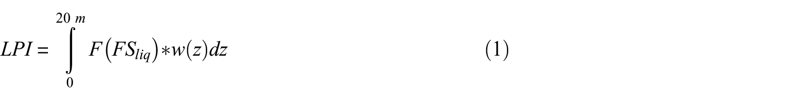
where z is the depth in meters, FS_liq is the factor of safety against liquefaction at depth z, F(FS_liq) = 1−FS_liq for FS_liq ≤ 1 and F(FS_liq) = 0 otherwise; and w is the depth-weighting factor, w(z) = 10–0.5 × z.

Based on the work by Ishihara (1985), Maurer et al. (2015b) proposed a modified LPI termed LPI_ISH that accounts for the crust thickness (H₁) and uses a different depth-weighting factor, w(z) = 25.56 × z⁻¹. The crust thickness parameter is defined in the work by Ishihara (1985) as the depth from the top of the soil to the first liquefiable layer. A third commonly used LDP is the liquefaction severity number (LSN) (van Ballegooy et al., 2014). The LSN is based on the predicted post-liquefaction volumetric strain, which is a function of FS_liq and relative density (Ishihara and Yoshimine, 1992) or FS_liq and the equivalent clean sand normalized CPT tip resistance (q_c_1Ncs) (Zhang et al., 2002).

Common for these three LDPs is that (1) they consider the top 20 m of the soil profile; (2) the layers closer to the soil surface have a greater weight than deeper soil layers; (3) they require an estimate of the FS_liq against liquefaction triggering; and (4) they require selection of a threshold index(s) to differentiate between surface manifestation severity levels. There are numerous liquefaction-triggering models that estimate FS_liq based on CPT data (e.g. Architectural Institute of Japan 2001; Boulanger and Idriss, 2016; Moss et al., 2006; Robertson and Wride 1998; Youd et al., 2001), all of which may yield somewhat different FS_liq. Therefore, LDPs are unique to the selected triggering model used, as discussed in the work by Maurer et al. (2015a). Likewise, Geyin and Maurer (2020) pointed out that the optimum threshold index is also dependent on the assumed misprediction consequences (i.e. is it worse to predict manifestation when it does not happen or to not predict manifestation when it does happen?).

A more recent method was proposed by Hutabarat and Bray (2022). Their model compares the liquefaction ejecta demand parameter (L_D) against the crust resistance parameter (C_R) to estimate the severity of liquefaction ejecta. This method is unique in that it specifically predicts the severity of liquefaction ejecta, whereas LPI, LPI_ISH, and LSN predict severity of liquefaction manifestation due to not only ejecta but also other forms of manifestation, such as cracking or settlement. L_D is a measure of the upward seepage pressure developed in a critical zone due to earthquake shaking and is a function of the excess hydraulic head (h_exc) and vertical hydraulic conductivity (k_v) of soils in the critical zone. L_D is estimated as:

r_{u} = {\begin{matrix} 1.0 & for F S_{liq} \leq 1.0 \\ 0.5 + \frac{si n^{- 1} (2 * {FS}_{liq}^{- 5} - 1)}{π} \\ 0 & for F S_{liq} \geq 3.0 \end{matrix} for 1.0 \leq F S_{liq} \leq 3.0

(2)

h_{exc} = \frac{r_{u} * σ_{v}'}{γ_{w}}

(3)

\frac{k_{v}}{k_{cs}} = 10^{(0.952 - 3.04 * I_{c})} / (3 * 10^{- 5}) for 1.0 \leq I_{c} \leq 3.27

(4)

L_{D} = {\begin{matrix} γ_{w} * \int_{z_{A}}^{z_{B}} \frac{k_{v}}{k_{c s}} * (h_{e x c} - h_{A}) d z & for h_{e x c} \geq h_{A} \\ 0 & otherwise \end{matrix}

(5)

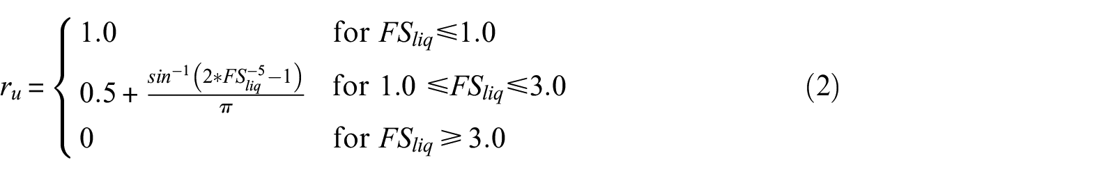
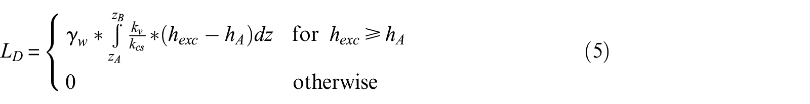
where r_u is the excess pore pressure ratio, σ’_v is the initial vertical effective stress, γ_w is the unit weight of water, I_c is the soil behavior type index, k_cs is the value of k_v for clean sand (I_c = 1.8), h_A is the value of h_exc at depth z required to produce artesian flow and is set equal to z, z_A is the depth from the ground surface to the top of the shallowest layer below the ground water table that has I_c < 2.6 and is at least 25 cm thick, and z_B is the depth from the ground surface to the top of the shallowest soil layer between z_A and 15 m with I_c > 2.6 and at least 25 cm thick.

C_R is a measure of the strength and thickness of the non-liquefiable crust layer and is estimated as:

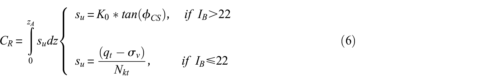
C_{R} = \int_{0}^{z_{A}} s_{u} dz {\begin{matrix} s_{u} = K_{0} * \tan (ϕ_{CS}), if I_{B} > 22 \\ s_{u} = \frac{(q_{t} - σ_{v})}{N_{kt}}, if I_{B} \leq 22 \end{matrix}

(6)

where s_u is the shear strength of the crust, K₀ is the coefficient of lateral earth pressure (assumed to be 0.5), $ϕ_{CS}$ is the critical state friction angle (assumed to be 33°), q_t is the CPT tip resistance, σ_v is the total stress, N_kt = 15, and I_B is the modified soil behavior type index (Robertson, 2016). For larger values of L_D and smaller values of C_R, the model predicts that the liquefaction ejecta severity increases. This method only considers soils in the top 15 m of a soil profile and was developed using FS_liq estimated from the Boulanger and Idriss (2016) triggering procedure at a probability level of 0.5. Hutabarat and Bray (2022) define threshold levels of L_D and C_R combinations that differentiate between liquefaction ejecta severity levels.

Data

The Global database (Geyin and Maurer, 2020) and the Canterbury database (Geyin et al., 2021) were used in this study. The Global database is a compilation of 275 liquefaction case histories from 21 earthquakes that occurred in nine countries. Geyin and Maurer (2020) compiled the Global database from existing literature. Older case histories were refined with information from newer studies, if available. Each case history consists of the peak ground acceleration (PGA), moment magnitude (M_w), ground water table depth (GWT), measured CPT tip resistance (q_c) and sleeve friction (f_s) at a given depth (z), latitude and longitude of the CPT, and a binary classification of whether surface manifestation due to liquefaction was observed or not. Geyin and Maurer (2020) also included thin layer-corrected q_c and f_s values according to the procedure of Boulanger and DeJong (2018); however, in this study, the original, uncorrected CPT data were used. Approximately 58% of the case histories in the Global database have observed surface manifestation and 42% do not.

The Canterbury database consists of 14,948 case histories from the M_w 7.1, September 4, 2010, Darfield earthquake, the M_w 6.2, February 22, 2011, Christchurch earthquake, and the M_w 5.7, February 14, 2016, Christchurch earthquake. The Canterbury database contains similar information as the Global database except the manifestation is classified as none, minor, moderate, or severe. To be consistent with the Global database, we reclassified all case histories with minor, moderate, and severe labels to “observed manifestation,” and those with none to “no observed manifestation.” The groundwater depth and the PGA values at individual CPT locations were estimated from regional models derived from measured data. Approximately 35% of the case histories in the Canterbury database have observed surface manifestation and 65% do not. Both databases only include case histories for free-field level ground conditions, and sites with lateral spreading were excluded in this study. None of the data from the Canterbury database is included in the Global database and vice versa. The Global database only includes one earthquake from New Zealand, the 1987 M_w = 6.6 Edgecumbe earthquake, which occurred on the North Island about 700 km from Christchurch. Figure 1 shows the marginal plots of pairs of PGA-M_w and GWT-LPI for both databases with their manifestation classifications.

Figure 1.

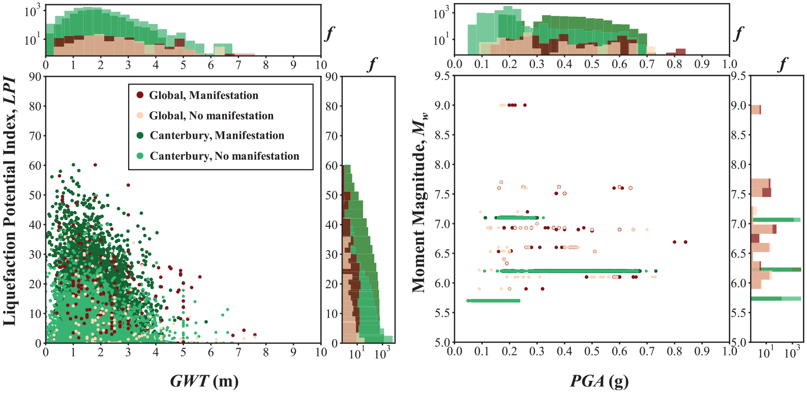
Selected parameters from the Global and Canterbury databases.

Methodology

CBR framework

CBR is a method where new problems are solved using the known solutions to old problems. CBR takes a design case and compares it to case histories in a database. It then finds the case history that is the most similar to the design case and uses the observed outcome of that case history as the predicted outcome of the design case (or the majority outcome of the most similar case histories). In the context of liquefaction manifestation modeling for this study, case histories are defined as a PGA, M_w, GWT, and CPT measurement for a given site and the corresponding outcome of observed liquefaction surface manifestation or not.

The essence of CBR is how to define how similar the case histories in the database are to the design case history. This is accomplished in two steps (Roberts and Engin, 2019). The first step is to compare a specific parameter of the design case to the same parameter of all the case histories in the database and calculate a similarity index for that parameter for each case history. This is then repeated for as many parameters as desired. The second step is to then calculate the overall similarity score for each case history as the weighted average of all the parameter-specific similarity indexes. The weights given to each parameter reflect their relative importance in predicting the correct result. This process is defined mathematically as:

S_{j} = \sum_{i = 1}^{n} I_{i, j} * w_{i}

(7)

where S_j is the overall similarity score for case history j, I_{i, j} is the similarity index for parameter i and case history j, w_i is the normalized weight for parameter i, and n is the total number of parameters used. The outcome of the case history with the largest similarity score or the majority outcome of case histories above a given threshold level is then used as the predicted outcome of the design case. Figure 2 provides a schematic overview of this process and presents some of the different meta-parameters tried as part of this study. The following sections describe the CBR framework and meta-parameters in more detail.

Figure 2.

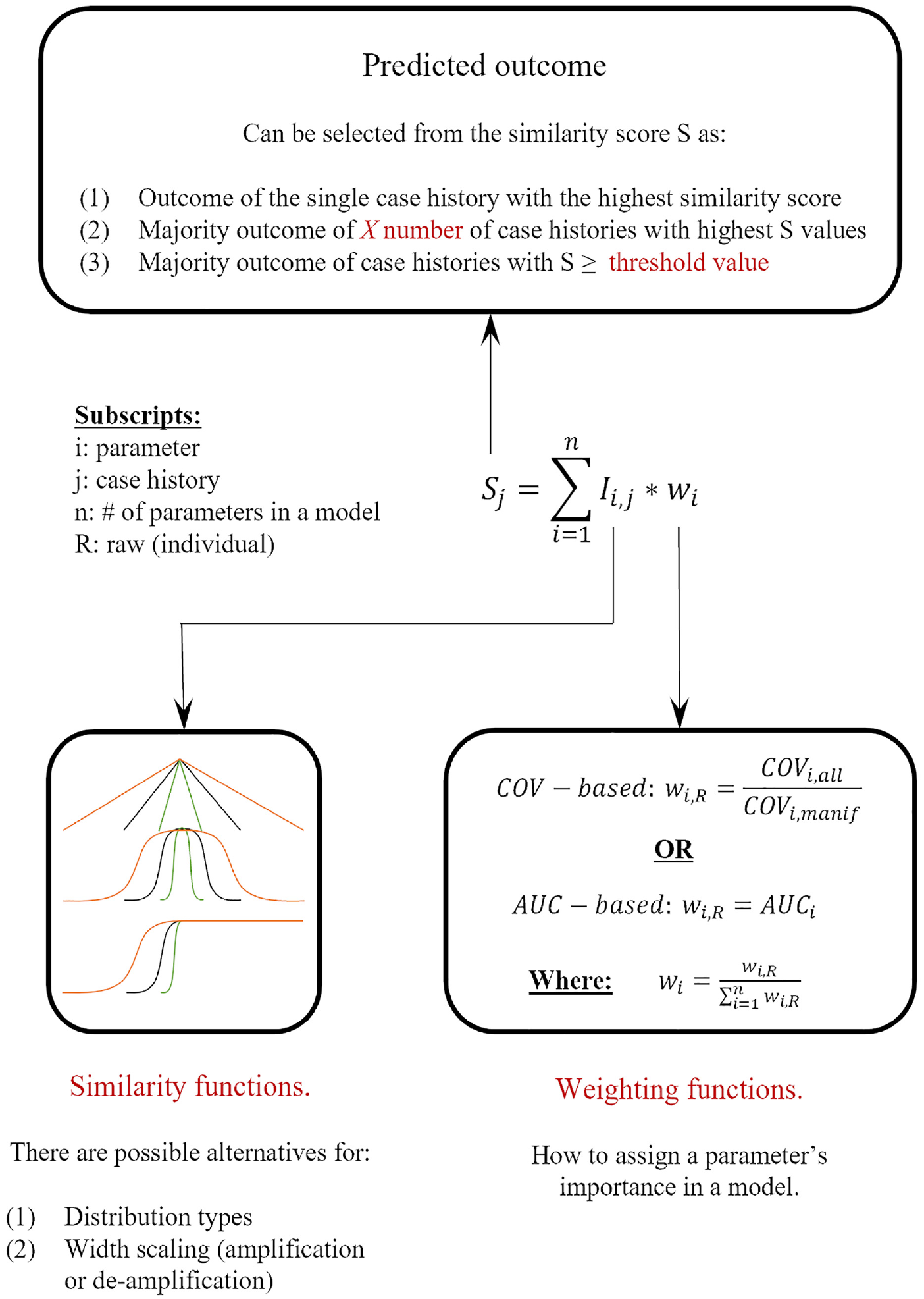
Schematic of the CBR framework employed in this study.

Similarity index

The similarity index (I) is estimated using a similarity function f(Z) that assigns a value based on the relative difference (Z) between the design case parameter (D) and the same parameter for the case history (C):

I_{i, j} = f (Z_{i, j}) = f ((D_{i, j} - C_{i, j}) / σ_{N, i})

(8)

where σ_N is a normalization coefficient to prevent differences in the magnitude of the different parameter values affecting the results. We tried three different similarity functions based on a normal distribution (base case), triangular distribution, and a modified normal distribution (Figure 3). When the design case parameter and the case history parameters are equal, the relative difference, Z, becomes zero and the similarity index equals one. The normal and triangular distributions decrease evenly on both sides of the peak, indicating that the larger the difference between the design case parameter and the case history parameter, the lower the similarity index (i.e. they are less similar). The modified normal distribution is the same as the normal distribution except the similarity index for one side of the curve is kept equal to one out to either + infinity or − infinity instead of decreasing to zero. The reasoning behind this function is that if a case history reported surface manifestation for PGA = X, then if the design case was exactly the same but PGA > X, this would also be assumed to result in surface manifestation. Or vice versa, if a case history reported no surface manifestation for PGA = X, then for a design case with similar parameters but PGA < X, one would also expect no surface manifestation. The direction of the modified normal distribution changes depending on whether the parameter has a positive or negative correlation with manifestation (e.g. PGA and GWT have opposite modification directions), and whether surface manifestation was observed or not.

Figure 3.

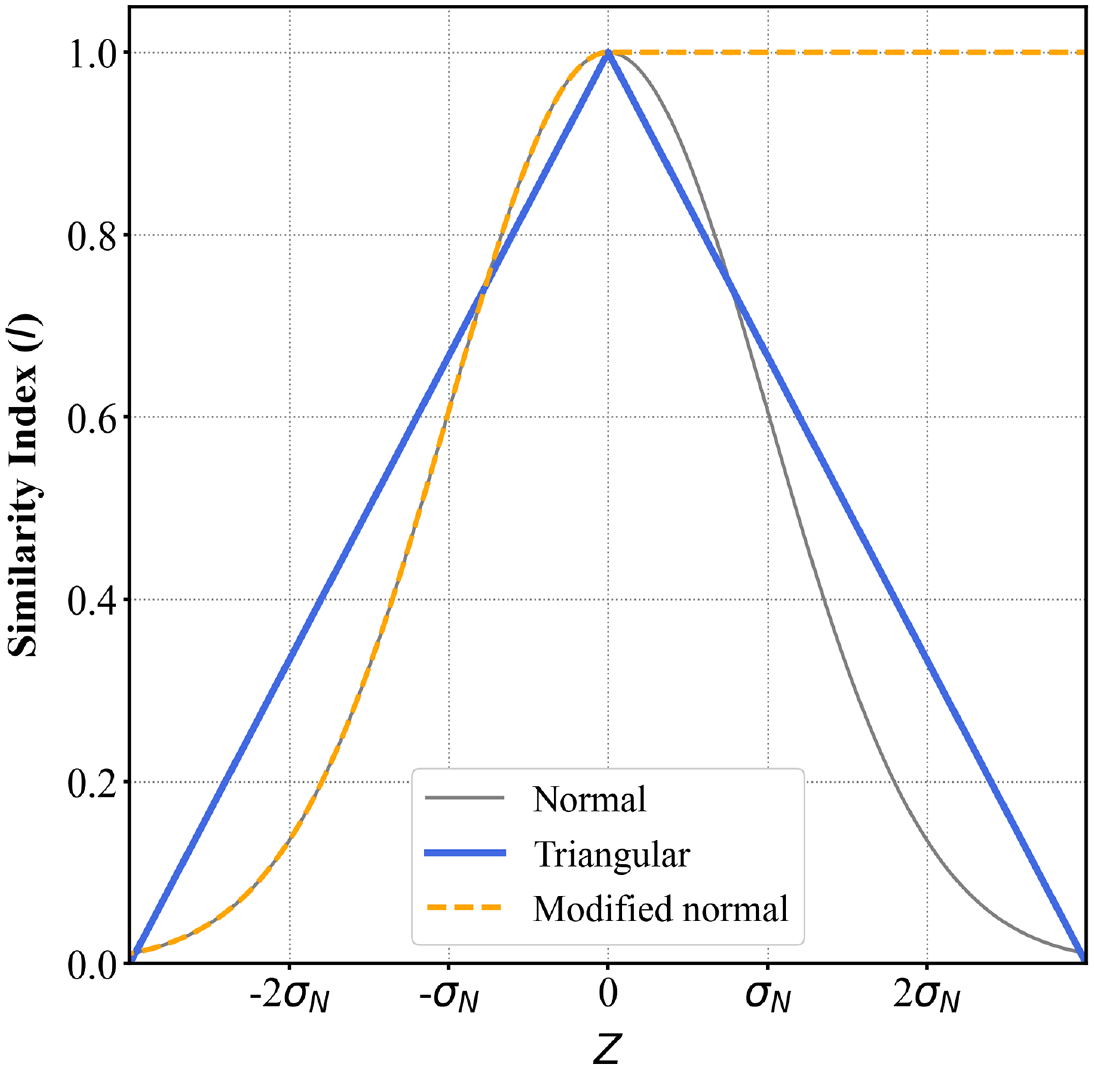
Similarity functions used in the CBR analyses.

We also tried three different values for the normalization coefficient (σ_N). We tried (1) the standard deviation of the given parameter for only the case histories with observed surface manifestations (σ_N = σ_manif; base case), similar to the work by Roberts and Engin (2019); (2) the amplified standard deviation (σ_N = A*σ_manif), which increases the width of the similarity function and gives a larger similarity index to values further from the design case value; and (3) the de-amplified standard deviation (σ_N = σ_manif /A), which narrows the similarity function and reduces the similarity index for values further from the design case value. In this work, A was arbitrarily selected to be 4 to see the effect of σ_N on the CBR results.

Weighting functions

The weight applied to each similarity index reflects the relative influence of that parameter in estimating correctly whether surface manifestation will occur or not compared to the other parameters used in the CBR analysis. We tried two different methods to estimate the weight. The first was the same as the work by Roberts and Engin (2019):

w_{i, R} = \frac{CO V_{i, all}}{CO V_{i, manif}}

(9)

w_{i} = \frac{w_{i, R}}{\sum_{i = 1}^{n} w_{i, R}}

(10)

where COV_{i, all} is the coefficient of variation of parameter i for all case histories, COV_{i, manif} is the coefficient of variation of parameter i for only case histories with observed surface manifestations, and w_iR is the raw weight. The raw weights are then normalized so that the sum of all the weights is equal to one. As a result of the normalization, the similarity score (S) has values between zero and one.

For the second method, we calculated the raw weight of each parameter (w_iR) as the area under (AUC) the receiver-operating-characteristic (ROC) curve. ROC curves plot the rate of true-positive predictions (R_TP) (i.e. manifestation is observed and predicted) against false-positive predictions (R_FP) (i.e. manifestations are not observed but are predicted to occur) when using different threshold values to differentiate the outcome. AUC is an objective and standardized metric used to evaluate the ability of a parameter to differentiate between two outcomes for different threshold values, and is commonly used in geoscience and geoengineering (e.g. Ju et al., 2020; Lin et al., 2021; Sarma et al., 2020; Upadhyaya et al., 2021, 2023). Figure 4 shows an example ROC curve and AUC for LPI using the Global database. Each point on the curve represents a different LPI threshold value. If LPI was a perfect predictor of liquefaction manifestation, then the curve would go from (0,0) to (0,1) to (1,1) and have an AUC = 1. Random guessing is equivalent to a straight line from (0,0) to (1,1) with an AUC = 0.5. The AUC therefore provides an estimate of the predictive power of each parameter individually to evaluate manifestation. The AUC values were taken as w_iR and then normalized as shown in Equation 10 to predict S values between zero and one.

Figure 4.

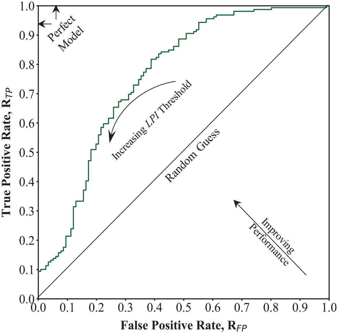
ROC curve using Global database and LPI as the diagnostic index.

Predictor parameters

To find the best CBR model to estimate liquefaction surface manifestation, we evaluated over 900 different predictor parameters. We included existing LDPs, such as LPI, LPI_ISH, LSN, L_D, C_R, and L_D/C_R described earlier. We calculated these parameters using FS_liq estimated by the CPT triggering model of Boulanger and Idriss (2016), as it presents one of the highest prediction efficacies (Geyin et al., 2020) and is widely used in practice.

Cubrinovski et al. (2019) found negligible difference in the LPI and LSN values for selected sites that had observed surface manifestation and no surface manifestation during the Canterbury earthquake sequence. They stated that the main differences between sites with observed surface manifestation compared to those with no observed surface manifestation were the presence of a vertically continuous liquefiable zone and the absence of a non-liquefiable crust. Therefore, we also evaluated parameters z_A, z_B, and z_A–z_B from the work by Hutabarat and Bray (2022). Parameter z_A is the depth from the ground surface to the top of the shallowest layer below the ground water table that has I_c < 2.6 and is at least 25 cm thick, and z_B is the depth from the ground surface to the top of the shallowest soil layer between z_A and 15 m with I_c > 2.6 and at least 25 cm thick. Parameter z_A represents the depth to the first layer susceptible to liquefaction, similar to the H₁ parameter defined in the work by Ishihara (1985). Parameter z_B is the depth to the bottom of the critical zone, and z_A–z_B is the thickness of the critical zone. Theoretically, for smaller values of z_A and larger values of z_A–z_B, the probability of liquefaction manifestation should increase. We also included the GWT as a proxy for the depth to the first susceptible layer, as this is a common parameter in regional methods (Zhu et al., 2017) and was readily available in the case history databases.

To represent the earthquake loading, we used PGA and M_w. Several studies (Kramer and Mitchell, 2006; Sideras, 2019) have found that the cumulative absolute velocity (CAV) is a better predictor of liquefaction than PGA. However, the case histories in the databases used in this study only include PGA and M_w; therefore, other earthquake loading parameters could not be assessed. In the future, other intensity measures could be calculated for the case histories and incorporated into the CBR method.

In addition to the above-listed predictor parameters, we also evaluated depth-dependent CPT-derived parameters. Table 1 lists these parameters and the reference where they are defined. Because these parameters are depth-dependent, we evaluated their mean, median, minimum, maximum, and standard deviation over depth intervals of 0–z_A, z_A–z_B, and 0–5, 0–10, 0–15, and 0–20 m for soils with I_c < 1.8 (clean sands), I_c < 2.6 (susceptible soils), and all soils irrespective of their liquefaction susceptibility. Soil unit weight values that are necessary to calculate some of these parameters were estimated using the CPT correlation of the work by Robertson and Cabal (2010). The factor of safety values were capped at a maximum of 10, which has an effect on the median, mean, standard deviation, and maximum values of FS_liq.

Table 1.

CPT-derived predictor parameters

Parameter	Name	Reference
D_R	Relative density	Idriss and Boulanger (2008)
Q_tn	Normalized tip resistance	Robertson (2009)
F_r	Sleeve friction ratio	Robertson (1990)
q_c1N	Overburden-corrected penetration resistance	Boulanger and Idriss (2016)
q_c1Ncs	Equivalent clean sand penetration resistance	Boulanger and Idriss (2016)
I_c	Soil behavior type index	Robertson and Wride (1998)
CRR_M ₌ _7.5,σ’v ₌ _1atm	Magnitude- and stress-normalized cyclic resistance ratio	Boulanger and Idriss (2016)
FS_liq	Factor of safety (at probability level of 15%)	Boulanger and Idriss (2016)
r_u	Excess pore pressure ratio	Hutabarat and Bray (2022)
h_exc	Excess hydraulic head	Hutabarat and Bray (2022)

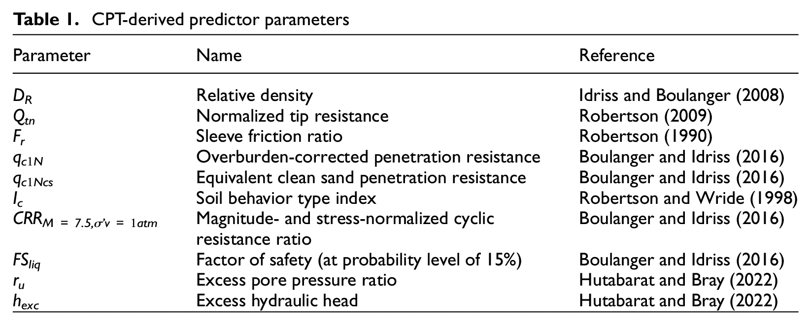
We included both the mean and median values because the median value is less affected by large outliers than the mean value. The standard deviations of parameters were included to try and capture the homogeneity (i.e. interbedded characteristics) of the soil profiles (Durante and Rathje, 2021). The more interbedded the soils are the larger the standard deviation and the more homogeneous they are the smaller the standard deviation. The values for the depth interval of 0–z_A represent the properties of the overlying crust, and the values for the depth interval of z_A–z_B represent the properties of the critical zone. We considered other generic depth intervals down to 20 m to see if these are better at capturing manifestation than parameters based on the critical zone or crust layer. Finally, values were also calculated filtering on I_c to see if parameters only for a given soil type controlled the response.

Some combinations of the CPT-derived parameters provide trivial results. These parameters were very poor predictors and were naturally filtered out in the regression analyses. For some case histories, some of the calculated parameters do not exist. For example, if there are no soils with I_c < 1.8 in the top 5 m, then all the parameters based on this filtering were replaced with an arbitrarily large number (e.g. 10,000). In this way, the CBR method can still match together case histories that do not have soils with I_c < 1.8 in the top 5 m for parameters based on this filtering. However, the CBR method will return a similarity index equal to zero when comparing to case histories that have at least a small layer with I_c < 1.8 in the top 5 m because the value calculated will be far from 10,000.

We also calculated the thickness of I_c < 1.8 and I_c < 2.6 over the depth intervals listed above and included them as predictor parameters. These parameters are zero if there are no soils meeting these criteria and therefore will give a high similarity index when compared with profiles where there are thin layers of soil meeting the filtering criteria. In addition, the thickness of I_c < 1.8 or 2.6 can also be used as a proxy to capture the finding in the work by Cubrinovski et al. (2019) that the thickness of liquefiable soil, even above or below the critical zone, can affect the manifestation response. These simple parameters do not, however, consider whether the liquefiable layers are continuous or not.

For the depth interval of 0–z_A (the overlying cap), we also calculated the thickness of I_c > 2.6 (cap-thick), which is more meaningful for this depth interval than the thickness of I_c less than a given threshold. Finally, we evaluated the thickness of FS_liq < 1.0 over the given depth intervals. The thickness of FS_liq < 1.0 is similar to LPI and LSN but simpler in form and is over different depth intervals rather than just the top 20 m.

Model development

To evaluate which combination of predictor parameters resulted in the best CBR model, we used Matthews Correlation Coefficient (MCC) as the goodness-of-fit measure (Matthews, 1975). MCC is a scalar value that measures the correlation between the true and predicted values:

MCC = \frac{TP * TN - FP * FN}{\sqrt{(TP + FP) * (TP + FN) * (TN + FP) * (TN + FN)}}

(11)

where TP is the number of true positives (manifestation is observed and predicted), TN is the number of true negatives (manifestation is not observed and not predicted), FP is the number of false positives (manifestation is not observed but predicted), and FN is the number of false negatives (manifestation is observed but not predicted). If MCC = 1, then the model predicts the correct response every time. If MCC = 0, then the model is no better than random guessing. The advantage of MCC over other classification metrics is that it is insensitive to class imbalance (e.g. more positive observations than negative or vice versa) and only predicts a high value if all four confusion matrix categories (TP, TN, FP, and FN) have good results. Another useful attribute is that the definition of positive and negative classes can be switched, and the score is the same. An inherent assumption in MCC is that reducing FP (over-conservative result) is just as important as reducing FN (unconservative result), which makes it an impartial metric.

To find the best combination of predictor parameters, we first tried all combinations of parameters for models with one or two parameters. This resulted in 938 one-parameter models and 439,453 two-parameter models. However, repeating this for models with three parameters was too computationally expensive (137,109,336 models). Therefore, we chose the best 175 predictor parameters based on the results of the one- and two-parameter models and evaluated all combinations of three-parameter models based on these 175 predictor parameters (877,975 models). Then, for the 100 best one-, two-, and three-parameter models, we performed a stepwise regression methodology using forward selection. In this approach, CBR was performed adding each remaining parameter one at a time to the base model. Then, the CBR model that gave the highest MCC value was retained, and the process repeated until the model had six parameters. Each model tried was then ranked according to MCC.

To find the optimum CBR parameters, we regressed on the Global database (training) and used the Canterbury database for validation (testing). We performed the regression with the Global database using a leave-one-out approach. In this approach, one case history was selected as the design case. The design case was then compared to the remaining case histories in the database using CBR to estimate whether surface manifestation would occur or not. This was repeated for each case history in the database. This ensured that every case history in the database was used as the design case one time. Finally, the results from all analyses were aggregated to compute the MCC.

We validated the CBR models developed using the Global database against the Canterbury database. For the validation, the case histories in the Canterbury database were the design cases and the Global database was the case history database. Each case history in the Canterbury database was evaluated against the Global database using a predefined set of parameters and weights derived from the Global database. Therefore, the validation is a true check as the CBR model has not seen the Canterbury data before and represents the scenario where a new earthquake occurs and the CBR model is used to predict liquefaction manifestation.

The base-case CBR models use the observed outcome of the case history with the single greatest similarity score as the predicted outcome for the design case. However, it is also possible to predict the outcome of the design case based on the observed outcomes of multiple of the most similar case histories. To explore this alternative method, we evaluated predicting the liquefaction manifestation outcome for the design case based on the observed outcomes of the 3, 5, or 10 case histories with the highest similarity scores, or the observed outcomes of all case histories with similarity scores greater than 0.75, 0.85, or 0.95. If half or more than half of the most similar case histories had observed liquefaction manifestation, then liquefaction manifestation was predicted for the design case. For example, if 6 of the 10 case histories with the highest similarity scores had observed liquefaction manifestation and 4 did not, then liquefaction manifestation was predicted for the design case. A useful benefit of this method is that probabilities of observing manifestation can also be calculated. Using the previous example, the probability of manifestation would be 60% because 6 of the 10 case histories with the highest similarity scores had observed manifestation, whereas 4 did not. If no case history had a similarity score above the 0.75, 0.85, or 0.95 threshold, then the observed outcome of the single case history with the highest similarity score was used, similar to the base case.

Results

Weights

The first step was to estimate the raw weight values for each parameter (w_R). As stated earlier, we tried two different sets of weights. The first set of weights was calculated as the coefficient of variation (COV) of all case histories for a given parameter divided by the COV of only those case histories with observed surface manifestation (COV_manif). The second set of weights was the AUC values of each parameter. Table 2 lists the AUC- and COV-derived weights (w_{R, COV} = COV / COV_manif) for the Global database. Only results for the five CPT-derived parameters with the highest AUC scores, five CPT-derived parameters with the highest w_{R, COV} values, and all existing LDP parameters and other parameters are shown. The naming convention for the CPT-derived parameters is generally based on four identifiers. The first part of the name is the CPT-derived parameter. The next identifier and first subscript is the depth interval over which the parameter is calculated. If it is a number, the depth interval is from zero to that depth in meters, if it is fsl, it signifies the depth to the first susceptible layer (0–z_a), and if it is crl, it signifies the critical zone (z_a–z_b). The next identifier in curly brackets is the I_c filter. The last identifier after the hyphen is the statistics being calculated for that parameter.

Table 2.

AUC and weights estimated from COV (w_{R, COV}) for the Global database. Only the five CPT-derived parameters with the highest AUC scores and w_{R, COV} values, and all non-CPT-derived parameters are shown

Type	Description	Notation	AUC	w_{R, COV}
CPT-based parameters with the greatest AUC	Cumulative thickness of layers with factor of safety less than unity, in the top 10 m	FSthick_{10_{all}}	0.77	1.429
	Mean r_u of all soils, in the top 10 m	Ru_{10_{all}-mean}	0.77	1.39
	Mean h_exc of all soils, in the top 10 m	hexc_{10_{all}-mean}	0.76	1.335
	Standard deviation of r_u of all soils, in top 10 m	Ru_{10_{all}-std}	0.76	1.958
	Median factor of safety of soils with I_c < 2.6, in the top 15 m	FS_{15_{Ic} _< _2.6}-median	0.75	0.838
CPT-based parameters with the greatest w_{R, COV}	Minimum factor of safety of soils with I_c < 2.6, in the top 10 m	FS_{10_{Ic} _< _2.6}-min	0.72	4.382
	Minimum F_r of all soils, in the top 5 m	Fr_{5_{all}-min}	0.63	4.052
	Minimum F_r of all soils, in the top 10 m	Fr_{10_{all}-min}	0.60	4.049
	Median CRR_Mw7.5-1 of soils with I_c < 2.6, in the critical zone	CRR_{crl_{Ic} _< _2.6}-median	0.61	4.024
	Minimum r_u of soils with I_c < 2.6, in z = (0, z_a)	Ru_{fsl_{Ic} _< _2.6}-min	0.50	3.865
Existing LDPs and other parameters	Liquefaction potential index	LPI	0.76	1.303
	Ishihara-inspired liquefaction potential index	LP_ISH	0.76	1.278
	Liquefaction severity number	LSN	0.71	1.156
	Normalized liquefaction ejecta demand	L_D/C_R	0.70	1.13
	Liquefaction ejecta demand	L_D	0.67	1.189
	Peak ground acceleration	PGA (g)	0.65	1.127
	Crust resistance	C_R	0.64	0.664
	Moment magnitude	Mw	0.61	1.065
	Thickness of soils with I_c > 2.6 in z = (0, z_a)	cap-thick (m)	0.60	1.023
	Depth of first liquefiable layer	z_A	0.59	1.168
	Groundwater table	GWT (m)	0.56	0.955
	Thickness of critical zone	z_A–z_B (m)	0.56	1.047

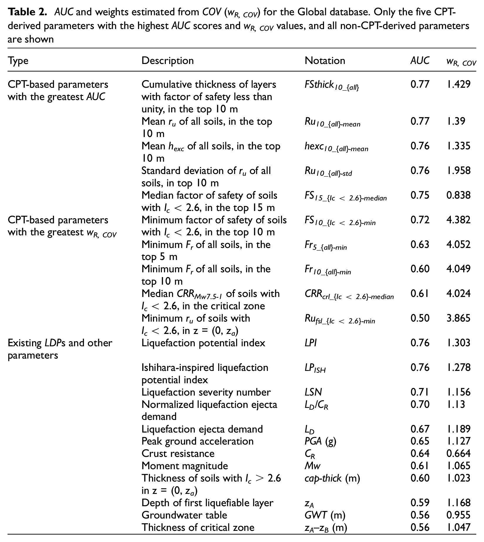
In general, the CPT-derived parameters with the largest AUC are based on r_u, FS_liq, and h_exc and the CPT-derived parameters with the largest w_{R, COV} are based on r_u, FS_liq, Fr, and CRR. For the non-CPT-derived parameters, LPI has the highest AUC and w_{R, COV} value.

Selected models

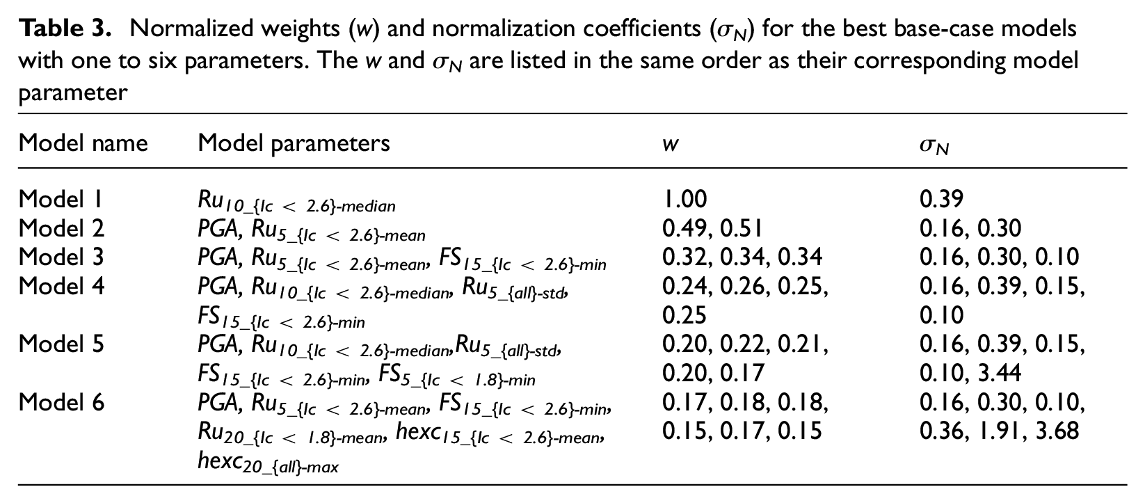
We first derived models using base-case meta-parameters, which are the AUC values as weights, a normal distribution for the similarity function with σ_N = σ_manif, and selecting only the observed outcome of the single most similar case history to predict the outcome of the design case. Table 3 lists the normalized weights (w) and normalization coefficients (σ_N) for the best models using one to six input parameters and base-case meta-parameters (Models 1–6). The w and σ_N are listed in the same order as their corresponding model parameter. The normalized weights are similar, showing that the parameters used in the selected models have similar AUC scores. Table 4 lists the MCC, true-negative rate (R_TN = TN/(TN + FP)), false-positive rate (R_FP = FP/(TN + FP)) false-negative rate (R_FN = FN/(TP + FN)), and true-positive rate (R_TP = TP/(TP + FN)) for each model. The larger the MCC, R_TN, and R_TP, and the smaller the R_FP and R_FN, the better the model. If R_TN is 0.5, this means the model is no better at predicting no manifestation cases than random guessing, and if R_TP is 0.5, this means the model is no better at predicting manifestation cases than random guessing. If either R_TN or R_TP is less than 0.5, this means the model is worse than random guessing. R_TN or R_TP values of 1 mean that the model predicts these cases perfectly (all cases in the training database are correctly predicted). The results present several interesting points, which are discussed below.

Table 3.

Normalized weights (w) and normalization coefficients (σ_N) for the best base-case models with one to six parameters. The w and σ_N are listed in the same order as their corresponding model parameter

Model name	Model parameters	w	σ_N
Model 1	Ru_{10_{Ic} _< _2.6}-median	1.00	0.39
Model 2	PGA, Ru_{5_{Ic} _< _2.6}-mean	0.49, 0.51	0.16, 0.30
Model 3	PGA, Ru_{5_{Ic} _< _2.6}-mean, FS_{15_{Ic} _< _2.6}-min	0.32, 0.34, 0.34	0.16, 0.30, 0.10
Model 4	PGA, Ru_{10_{Ic} _< _2.6}-median, Ru_{5_{all}-std}, FS_{15_{Ic} _< _2.6}-min	0.24, 0.26, 0.25, 0.25	0.16, 0.39, 0.15, 0.10
Model 5	PGA, Ru_{10_{Ic} _< _2.6}-median,Ru_{5_{all}-std}, FS_{15_{Ic} _< _2.6}-min, FS_{5_{Ic} _< _1.8}-min	0.20, 0.22, 0.21, 0.20, 0.17	0.16, 0.39, 0.15, 0.10, 3.44
Model 6	PGA, Ru_{5_{Ic} _< _2.6}-mean, FS_{15_{Ic} _< _2.6}-min, Ru_{20_{Ic} _< _1.8}-mean, hexc_{15_{Ic} _< _2.6}-mean, hexc_{20_{all}-max}	0.17, 0.18, 0.18, 0.15, 0.17, 0.15	0.16, 0.30, 0.10, 0.36, 1.91, 3.68

Table 4.

Matthews Correlation Coefficient (MCC), true-negative rate (R_TN), false-positive rate (R_FP), false-negative rate (R_FN), and true-positive rate (R_TP) for the best base-case models with one to six parameters

Model name	Model parameters	MCC	R_TN	R_FP	R_FN	R_TP
Model 1	Ru_{10_{Ic} _< _2.6}-median	0.384	0.61	0.39	0.23	0.77
Model 2	PGA, Ru_{5_{Ic} _< _2.6}-mean	0.461	0.67	0.33	0.21	0.79
Model 3	PGA, Ru_{5_{Ic} _< _2.6}-mean, FS_{15_{Ic} _< _2.6}-min	0.517	0.73	0.27	0.21	0.79
Model 4	PGA, Ru_{10_{Ic} _< _2.6}-median, Ru_{5_{all}-std}, FS_{15_{Ic} _< _2.6}-min	0.581	0.79	0.21	0.21	0.79
Model 5	PGA, Ru_{10_{Ic} _< _2.6}-median, Ru_{5_{all}-std}, FS_{15_{Ic} _< _2.6}-min, FS_{5_{Ic} _< _1.8}-min	0.593	0.78	0.22	0.19	0.81
Model 6	PGA, Ru_{5_{Ic} _< _2.6}-mean, FS_{15_{Ic} _< _2.6}-min, Ru_{20_{Ic} _< _1.8}-mean, hexc_{15_{Ic} _< _2.6}-mean, hexc_{20_{all}-max}	0.574	0.74	0.26	0.17	0.83

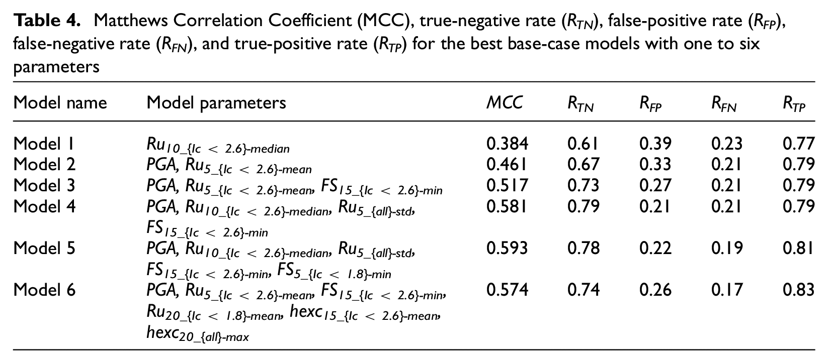
As the number of input parameters increases, the MCC increases up until five parameters, and decreases for the six-parameter model. This is most likely because adding more parameters decreases the weight of the other more influential parameters. Therefore, simply adding more parameters and making the model more complex does not necessarily result in a better model. Moreover, the model with only one parameter already has an R_TP = 0.77. Adding more parameters only marginally increases this value to 0.83. However, adding more parameters significantly increases the proportion of true negatives, from 0.61 to 0.79.

All six of the models in Table 3 consist of one or more of PGA, r_u, FS_liq, and h_exc. This agrees well with the results shown in Table 2, where these parameters have the highest AUC values. FS_liq is a direct indicator of liquefaction triggering and therefore a strong predictor of liquefaction manifestation. Parameters r_u and h_exc are correlated to FS_liq (r_u is a function of FS_liq and h_exc is a function of r_u and σ’_v) and therefore also performed well. It is interesting, however, that other parameters such as LPI, LPI_ish, or LSN, which are also functions of FS_liq, and other factors such as crust thickness and depth did not provide better models. These results may be attributable to the regional depth-weighting algorithms embedded into the existing LDPs not performing well for a Global database. It is expected that manifestation models perform better with the implementation of regionalized w(z), magnitude scaling factors (MSF), and stress reduction factors (r_d), as highlighted in the work by Green (2022). In addition, none of the models includes parameters based on the depth interval of the crust (0–z_A) or the critical zone (z_A–z_B), which we expected to be better predictors than the other depth intervals. Finally, Models 1 and 2 only use CPT data over the top 10 and 5 m, respectively, and Models 4–5 only use CPT data over the top 15 m. This is in contrast to LPI, LPI_ish, or LSN, which take weighted averages over the top 20 m, but similar to the model proposed in the work by Hutabarat and Bray (2022), which only considers the top 15 m of a soil profile.

Regional models

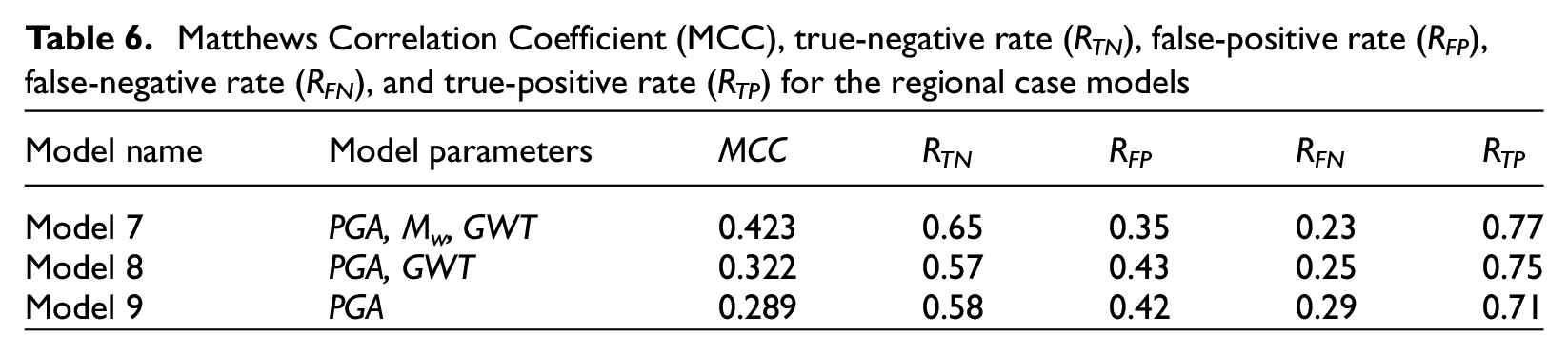
In addition to the best-fit models presented above, we explored three alternative models based only on PGA, M_w, and GWT to evaluate the ability of CBR to predict liquefaction manifestation with limited input parameters. These models could therefore be used for regional analyses where geotechnical data are sparse. Table 5 lists the normalized weights (w) and normalization coefficients (σ_N) for three models (Models 7–9) using only these parameters, and Table 6 lists the results. The best model uses all three parameters and provides a similar fit to the data as the two-parameter model listed in Table 4 (Model 2).

Table 5.

Normalized weights (w) and normalization coefficients (σ_N) for the regional models. The w and σ_N are listed in the same order as their corresponding model parameter

Model name	Model parameters	w	σ_N
Model 7	PGA, Mw, GWT	0.33, 0.36, 0.31	0.60, 0.16, 1.45
Model 8	PGA, GWT	0.54, 0.46	0.16, 1.45
Model 9	PGA	1.00	0.16

Table 6.

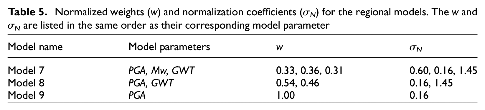
Matthews Correlation Coefficient (MCC), true-negative rate (R_TN), false-positive rate (R_FP), false-negative rate (R_FN), and true-positive rate (R_TP) for the regional case models

Model name	Model parameters	MCC	R_TN	R_FP	R_FN	R_TP
Model 7	PGA, M_w, GWT	0.423	0.65	0.35	0.23	0.77
Model 8	PGA, GWT	0.322	0.57	0.43	0.25	0.75
Model 9	PGA	0.289	0.58	0.42	0.29	0.71

Validation

The models were validated against the Canterbury database. Each case history in the Canterbury database was compared to the Global database using CBR and the models described above. Table 7 presents the results of the validation for each of the models. Similar to the model development, as the number of input parameters increases, the MCC generally increases. However, the MCC values for the validation are less than the values found when developing the models, which is expected, because the models were not trained on the Canterbury data. The maximum true-negative rate (rate that manifestation is not observed and not predicted) is 0.76 using the models with one or six parameters. The maximum true-positive rate (rate that manifestation is observed and predicted) is 0.72 using the five-parameter model.

Table 7.

Model results validated against the Canterbury database

Model name	Model parameters	MCC	R_TN	R_FP	R_FN	R_TP
Model 1	Ru_{10_{Ic} _< _2.6}-median	0.311	0.76	0.24	0.45	0.55
Model 2	PGA, Ru_{5_{Ic} _< _2.6}-mean	0.356	0.68	0.32	0.31	0.69
Model 3	PGA, Ru_{5_{Ic} _< _2.6}-mean, FS_{15_{Ic} _< _2.6}-min	0.392	0.72	0.28	0.31	0.69
Model 4	PGA, Ru_{10_{Ic} _< _2.6}-median, Ru_{5_{all}-std}, FS_{15_{Ic} _< _2.6}-min	0.389	0.73	0.27	0.32	0.68
Model 5	PGA, Ru_{10_{Ic} _< _2.6}-median, Ru_{5_{all}-std}, FS_{15_{Ic} _< _2.6}-min, FS_{5_{Ic} _< _1.8}-min	0.427	0.72	0.28	0.28	0.72
Model 6	PGA, Ru_{5_{Ic} _< _2.6}-mean, FS_{15_{Ic} _< _2.6}-min, Ru_{20_{Ic} _< _1.8}-mean, hexc_{15_{Ic} _< _2.6}-mean, hexc_{20_{all}-max}	0.435	0.76	0.24	0.32	0.68
Model 7	PGA, Mw, GWT	0.108	0.59	0.41	0.48	0.52
Model 8	PGA, GWT	0.179	0.58	0.42	0.39	0.61
Model 9	PGA	0.233	0.65	0.35	0.41	0.59

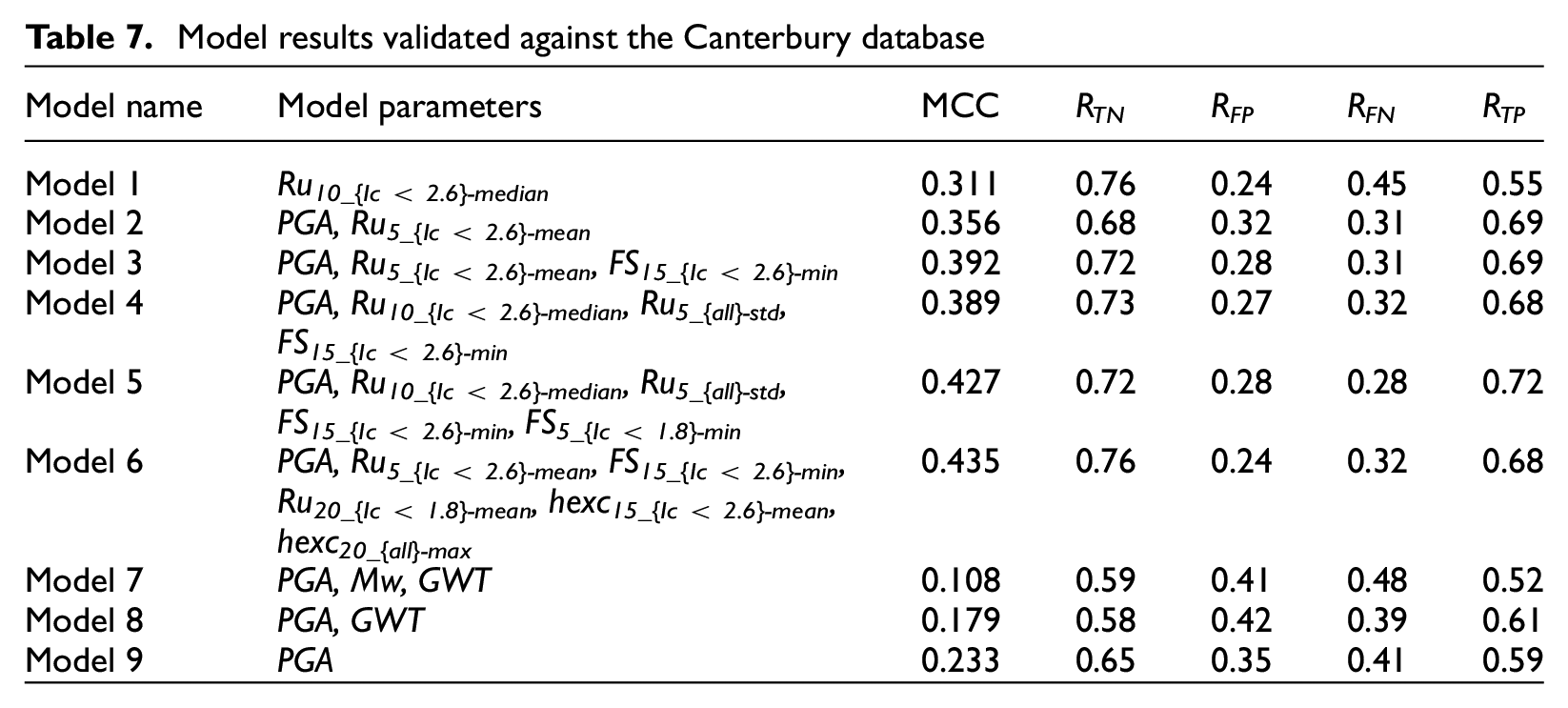
The three alternative models that do not require CPT data have lower MCC scores as well, which is expected. However, the model with only PGA performs the best, while the model with PGA, M_w, and GWT performs the worst of the three. This is opposite to the trend seen when developing the models, where the model with PGA, M_w, and GWT performed the best and PGA by itself was the worst. This shows that the regional CBR models are sensitive to the database used to perform the CBR calculation and may not provide reliable results when extrapolated to design cases outside the case history database.

Discussion

Effect of model meta-parameters

As discussed in the “Methodology” section, we evaluated several meta-parameters of the CBR model. These meta-parameters included (1) weighting functions based on either the AUC (base case) or the ratio of the COV of a given parameter for all case histories to the COV of the parameter for only the case histories with observed surface manifestation (w_{R, COV}); (2) similarity function based on either a normal distribution (base case), triangular distribution, or a normal distribution with one half of the distribution equal to one (modified normal); (3) similarity function based on a normal distribution with a standard deviation calculated as the standard deviation of the given parameter for only the case histories with observed surface manifestations (σ_N = σ_manif, base case), or σ_N multiplied or divided by four, and; (4) using only the single most similar case history (base case) to predict the outcome, the majority outcome of the 3, 5, or 10 most similar case histories, or the majority outcome of all case histories with similarity scores greater than 0.75, 0.85, or 0.95 together to predict the outcome.

Table 8 presents the MCC for the models given in Tables 4 and 6 for the base case and each of the different meta-parameter variations trained on the Global database. There is no one change in meta-parameters that consistently gives the best MCC for each model, and the base-case meta-parameters do not give the best MCC for each model either. The difference in MCC ranges from −0.38 to + 0.06. This result could change if the best models were initially derived using the change in the meta-parameters, or if multiple meta-parameters were changed simultaneously; however, this is outside the scope of the current study.

Table 8.

MCC values for different meta-parameters trained on the Global database. The italic and bold numbers are the largest MCC per model

Meta-parameter	Model name
	1	2	3	4	5	6	7	8	9
Base case	0.38	0.46	0.52	0.58	0.59	0.57	0.42	0.32	0.29
S > 0.75	0.42	0.32	0.39	0.45	0.47	0.46	0.19	0.22	0.20
S > 0.85	0.38	0.38	0.45	0.44	0.42	0.41	0.26	0.31	0.20
S > 0.95	0.41	0.36	0.39	0.50	0.44	0.47	0.23	0.11	0.19
Best 3	0.33	0.42	0.48	0.46	0.43	0.43	0.34	0.35	0.11
Best 5	0.38	0.47	0.41	0.35	0.33	0.49	0.30	0.22	0.20
Best 10	0.38	0.43	0.45	0.45	0.39	0.50	0.26	0.28	0.20
COV weights	0.38	0.45	0.52	0.57	0.58	0.58	0.42	0.32	0.29
De-amplification	0.38	0.46	0.48	0.53	0.56	0.63	0.44	0.31	0.29
Amplification	0.38	0.46	0.53	0.59	0.58	0.57	0.42	0.32	0.29
Tail distribution	0.40	0.23	0.24	0.20	0.22	0.27	0.21	0.29	0.23
Triangle distribution	0.38	0.45	0.50	0.58	0.55	0.60	0.44	0.36	0.29

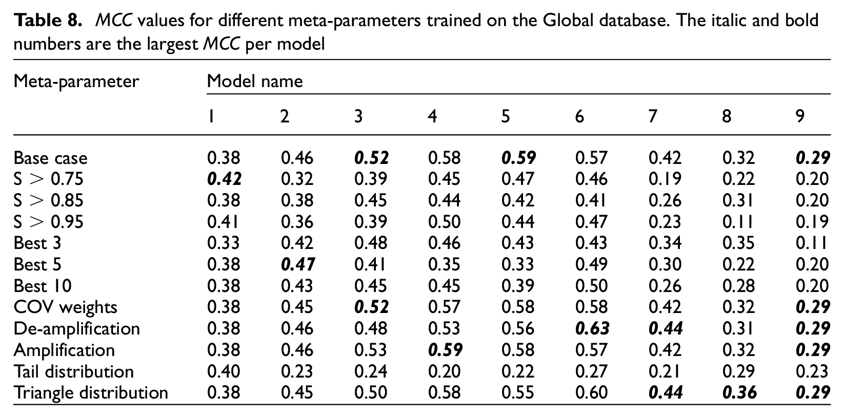
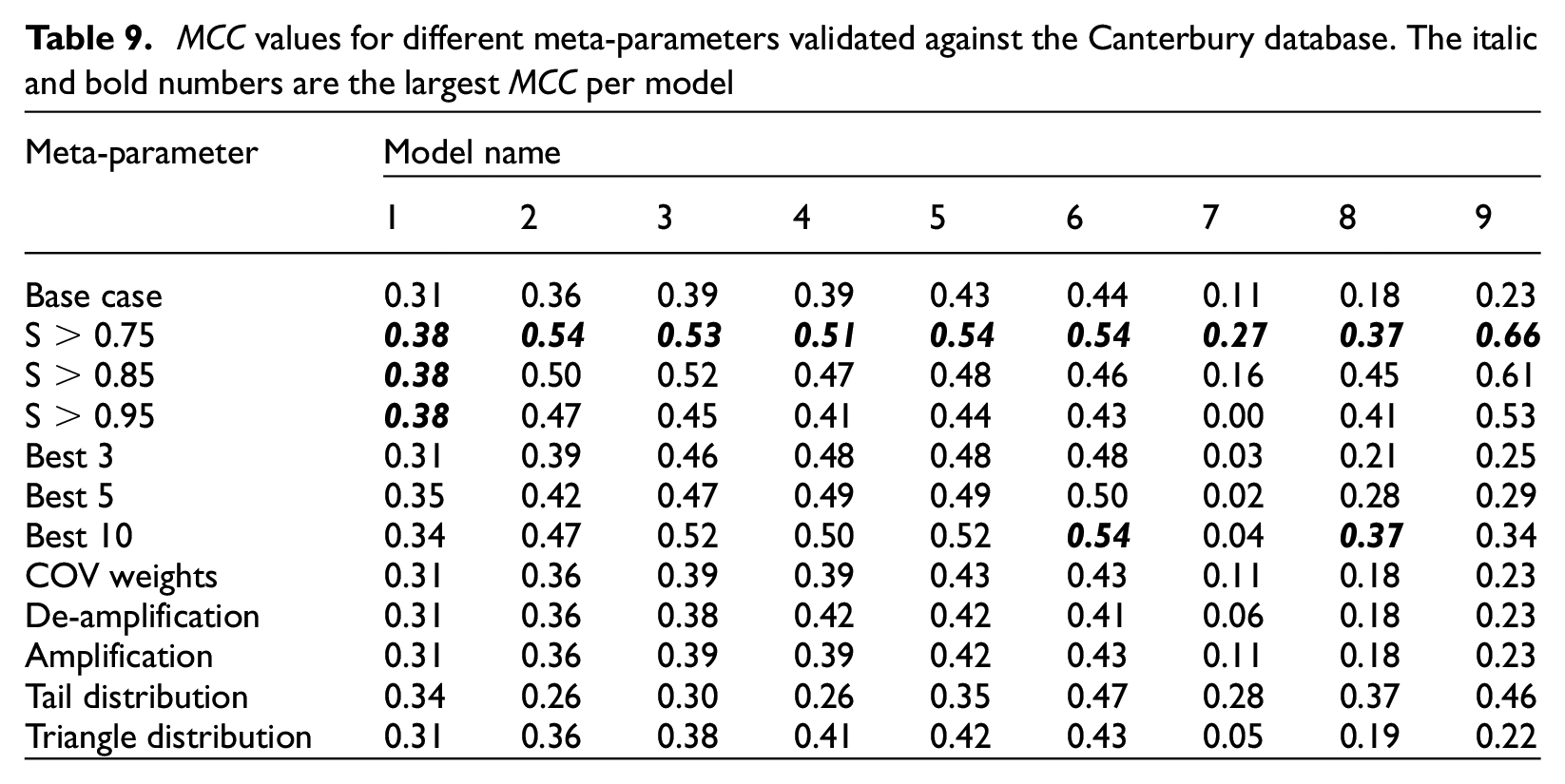
Table 9 presents the MCC for the same models as in Table 8 but validated against the Canterbury database. For the validation exercise, taking the majority outcome of all case histories with a similarity score > 0.75 provides a consistently better MCC for all the models tested. The difference is significant, with an increase in the MCC of 0.43 for the model with only PGA (Model 9) and an increase in more than 0.10 for all other models except Model 1. This could be because the Canterbury database represents a distinct set of case histories that do not match any one event or case history in the Global database. As a result, taking all the most similar case histories above a threshold (S > 0.75) and taking the majority outcome ensure a more robust result than simply taking the single case history with the highest similarity score.

Table 9.

MCC values for different meta-parameters validated against the Canterbury database. The italic and bold numbers are the largest MCC per model

Meta-parameter	Model name
	1	2	3	4	5	6	7	8	9
Base case	0.31	0.36	0.39	0.39	0.43	0.44	0.11	0.18	0.23
S > 0.75	0.38	0.54	0.53	0.51	0.54	0.54	0.27	0.37	0.66
S > 0.85	0.38	0.50	0.52	0.47	0.48	0.46	0.16	0.45	0.61
S > 0.95	0.38	0.47	0.45	0.41	0.44	0.43	0.00	0.41	0.53
Best 3	0.31	0.39	0.46	0.48	0.48	0.48	0.03	0.21	0.25
Best 5	0.35	0.42	0.47	0.49	0.49	0.50	0.02	0.28	0.29
Best 10	0.34	0.47	0.52	0.50	0.52	0.54	0.04	0.37	0.34
COV weights	0.31	0.36	0.39	0.39	0.43	0.43	0.11	0.18	0.23
De-amplification	0.31	0.36	0.38	0.42	0.42	0.41	0.06	0.18	0.23
Amplification	0.31	0.36	0.39	0.39	0.42	0.43	0.11	0.18	0.23
Tail distribution	0.34	0.26	0.30	0.26	0.35	0.47	0.28	0.37	0.46
Triangle distribution	0.31	0.36	0.38	0.41	0.42	0.43	0.05	0.19	0.22

Comparison with existing models

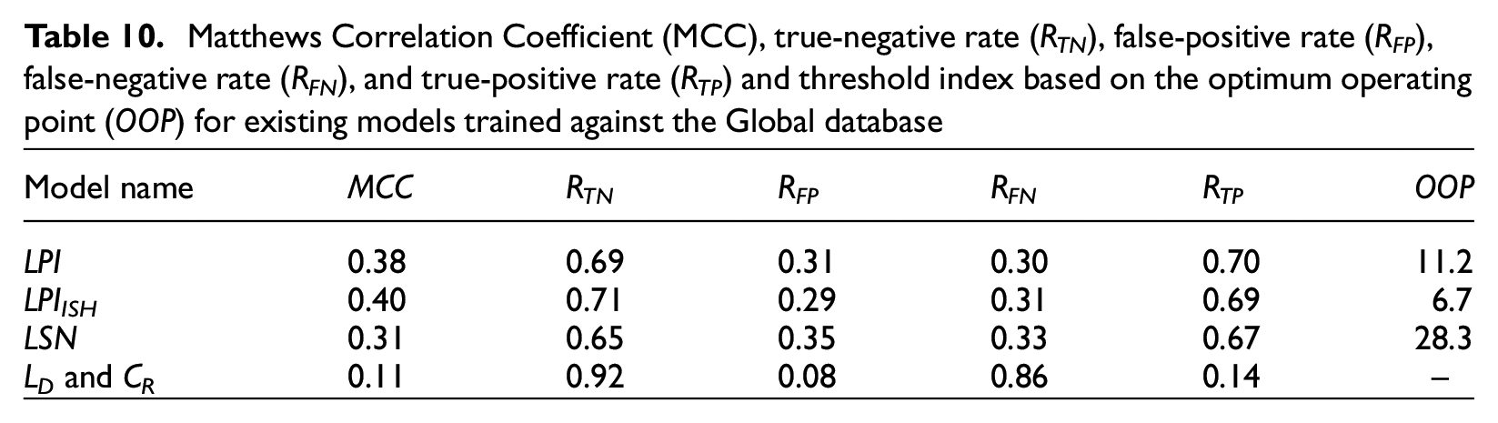
To understand the performance of the CBR models, we compared them with existing models. Figure 5 presents confusion matrices for LPI against the Global database and the Canterbury database. Confusion matrices are simply a graphical representation of R_TN, R_FP, R_FN, and R_TP. In addition, Tables 10 and 11 list the MCC, R_TN, R_FP, R_FN, and R_TP when using LPI, LPI_ISH, LSN, and the method of Hutabarat and Bray (2022) (L_D and C_R) against the Global database and the Canterbury database, respectively. For LPI, LPI_ISH, and LSN, threshold values of 11.2, 6.7, and 28.3 were used. These threshold values were chosen as the optimum operating point (OOP) obtained from ROC analyses using the Global database. The OOP is the best (optimum) threshold value that minimizes both the false-positive and false-negative counts. Therefore, using the OOP as a threshold assumes the cost of false positives is the same as false negatives. We then used the OOP value obtained from the Global database against the Canterbury database. This is similar to the validation of the CBR models and what would be done in practice if a new earthquake occurred and these LDPs were applied. For the Hutabarat and Bray (2022) model, we classified all cases in the “None” category (C_R, L_D pair below the line defined as (0, 2.5), (100, 2.5) and (250, 25)) as no manifestation and the rest as manifestation. There are a couple of key points that stand out when comparing the predictive capabilities of the existing models to the CBR models.

Figure 5.

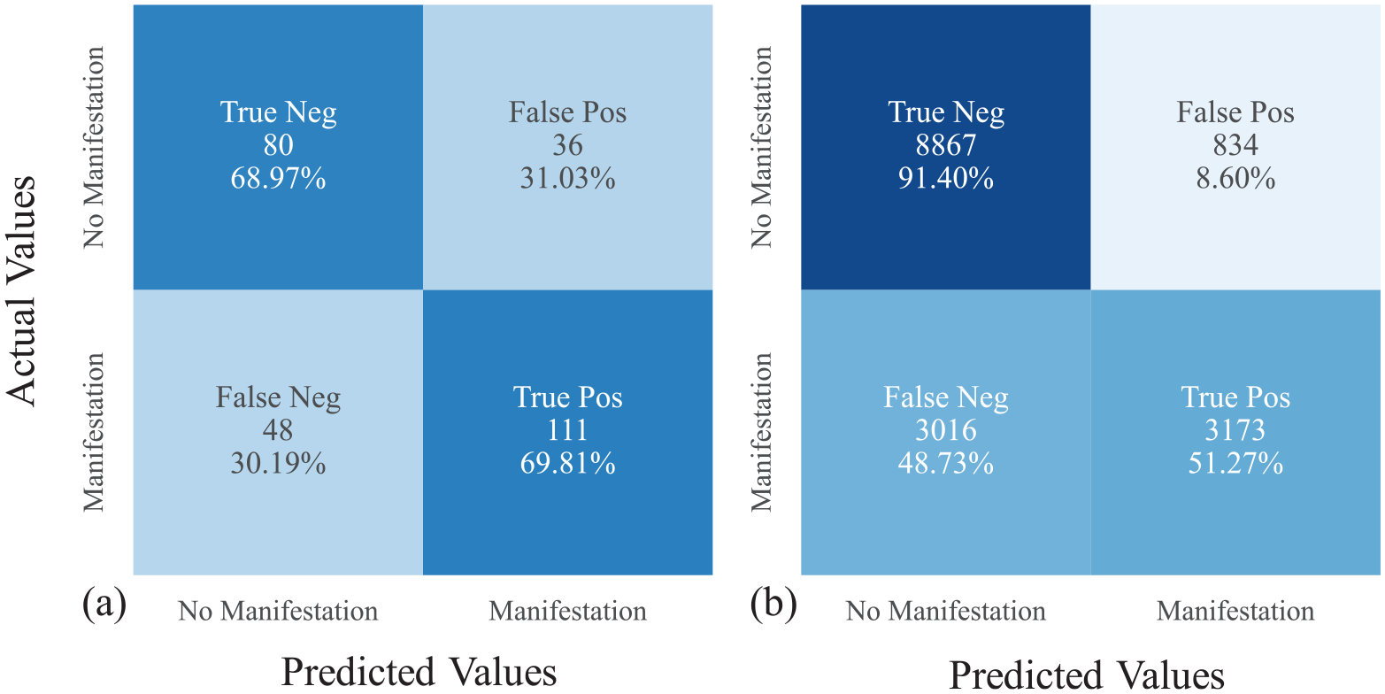
Confusion matrix for LPI using the Boulanger and Idriss (2016) triggering method for the (a) Global database and LPI threshold = 11.2 (MCC = 0.38) and (b) Canterbury database and LPI threshold = 11.2 (MCC = 0.48).

Table 10.

Matthews Correlation Coefficient (MCC), true-negative rate (R_TN), false-positive rate (R_FP), false-negative rate (R_FN), and true-positive rate (R_TP) and threshold index based on the optimum operating point (OOP) for existing models trained against the Global database

Model name	MCC	R_TN	R_FP	R_FN	R_TP	OOP
LPI	0.38	0.69	0.31	0.30	0.70	11.2
LPI_ISH	0.40	0.71	0.29	0.31	0.69	6.7
LSN	0.31	0.65	0.35	0.33	0.67	28.3
L_D and C_R	0.11	0.92	0.08	0.86	0.14	–

Table 11.

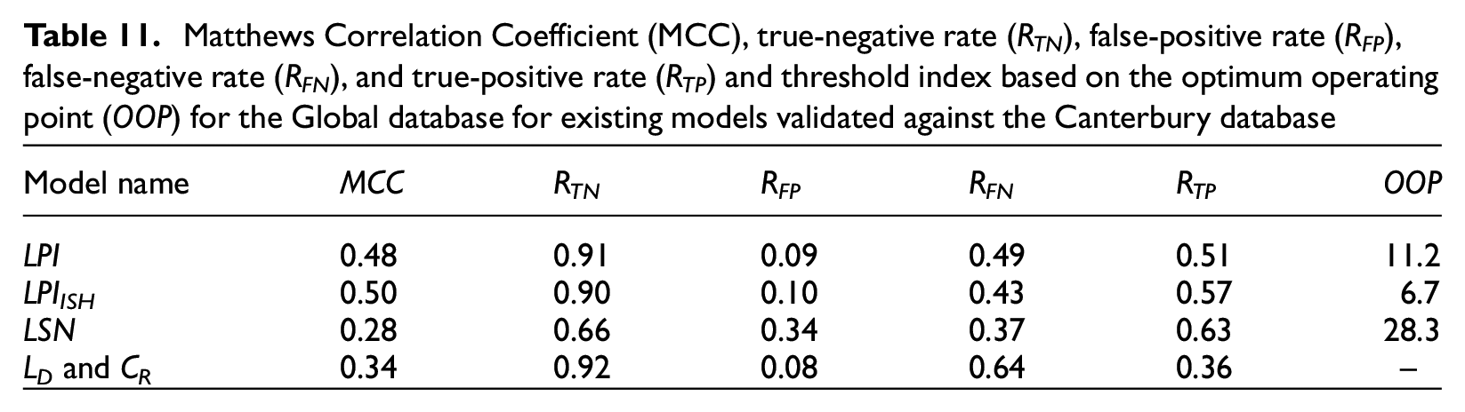
Matthews Correlation Coefficient (MCC), true-negative rate (R_TN), false-positive rate (R_FP), false-negative rate (R_FN), and true-positive rate (R_TP) and threshold index based on the optimum operating point (OOP) for the Global database for existing models validated against the Canterbury database

Model name	MCC	R_TN	R_FP	R_FN	R_TP	OOP
LPI	0.48	0.91	0.09	0.49	0.51	11.2
LPI_ISH	0.50	0.90	0.10	0.43	0.57	6.7
LSN	0.28	0.66	0.34	0.37	0.63	28.3
L_D and C_R	0.34	0.92	0.08	0.64	0.36	–

All the base models except Models 1, 8, and 9 have higher MCC than LPI, LPI_ISH, LSN, and the method of Hutabarat and Bray (2022) when using the Global database. This may seem trivial because the CBR models were trained against the Global database, but then so were LPI, LPI_ISH, and LSN. What this result shows then, is that when using the same input data and when trained on the same database of case histories, CBR can generate models with better predictive power than existing models. The Hutabarat and Bray (2022) model has a low R_TP value because it was developed to estimate only manifestation due to ejecta, and not other forms of manifestation, such as cracking or settlement, which are included in the Global database. Therefore, even if it correctly predicts cases with ejecta manifestation, it misses other forms of manifestation because it was not strictly developed to predict their occurrence.

When validated against the Canterbury database, Models 2–6 still have higher MCC than LSN and the method of Hutabarat and Bray (2022). However, LPI and LPI_ISH have higher MCC than all the base-case CBR models. This is only for the base-case models. If we compare the CBR models when taking the majority outcome of all case histories with similarity scores greater than 0.75 to predict the outcome, Models 4, 5, and 6 have higher MCC for both the training database (Global database) and the validation database (Canterbury) than the existing models (MCC = 045, 0.47, and 0.46 for the Global database and MCC = 0.51, 0.54, and 0.54 for the Canterbury database for Models 4, 5, and 6, respectively, compared to MCC = 0.4 and 0.5 for LPI_ISH). These results show that the CBR method has the potential to generate models with greater predictive capabilities than existing models using the same input data, even when validated against previously unseen data.

When using the OOP derived for the Global database against the Global database, the R_TN and R_TP values reach about 70% for both LPI and LPI_ISH. However, employing the same OOP against the Canterbury database causes R_TP values to decrease to 51% and 57% for LPI and LPI_ISH, respectively, while the R_TN increases to 91% and 90%. This is because the optimum threshold values for the Canterbury database are lower than for the Global database. As a result, true manifestation cases are incorrectly predicted to be no manifestation while almost all the no manifestation cases are correctly predicted. Therefore, even though the MCC value actually increases for LPI and LPI_ISH, the R_TP is less than all the base-case models except Models 1 and 7 when validated against the Canterbury model. When validated against the Canterbury database the MCC for LSN is about the same as for the Global database. The Hutabarat and Bray (2022) method has a higher MCC for the Canterbury database than the Global database, which is expected because it was developed based on case histories from the Canterbury sequence.

Advantages and practical implications of CBR

Potential advantages of the CBR method over traditional LDPs is that CBR does not require the definition of a threshold value to differentiate between surface manifestation. This makes CBR easier to use and more consistent in practice. In addition, when using the observed outcomes of multiple of the most similar case histories to predict the outcome of the design case, a probability of liquefaction manifestation occurrence can be predicted. CBR models also inherently merge liquefaction susceptibly, triggering, and manifestation. As a result, the level of accuracy is clearly defined for the entire liquefaction analysis, as opposed to the present state-of-practice where susceptibility, triggering, and manifestation models developed by various authors and separate datasets are often used together, and the collective accuracy of these different combinations is unknown. Finally, compared with other Artificial Intelligence methods, such as ANN that can feel like a black box for many, CBR is a fully transparent method that allows users to follow the reasoning on every level. This makes it easier to use in practice and easier to understand when aberrant results are predicted.

The main practical implication of these CBR models is to determine if surface manifestation, such as settlement, lateral spreading, cracking, or sand boils will occur or not. This is important for preliminary site investigations and land use planning. CBR models for manifestation could also be used in conjunction with triggering models to assess liquefaction hazard. Potential applications of the CBR models include site-specific liquefaction analyses where CPT data are available, regional analyses where CPT data are unavailable, or when CPT data are depth-restricted. For example, along pipeline and cable routes, CPT data are often only collected over the top 5 m to evaluate pipe–soil interaction and reduce costs. This study showed that CBR models (e.g. Model 2) can be developed that only require CPT data over the top 5 m and still have a comparable prediction success rate (i.e. ~70%) as existing models that require the top 20 m of CPT data.

Limitations of CBR

One of the main limitations of the CBR method is that it is dependent on the case history database used to develop it, even more so than traditionally derived empirical models. This is because unlike traditional models that identify trends in the data that can then be extrapolated, CBR selects the result of the most similar case history. This is a strength when the trends are highly nonlinear and not easy to fit with traditional functional forms. However, when used with design cases outside the parameter space of the case histories in the database, CBR could provide poor results. This will be seen by a low similarity score. As a result, when using CBR, the similarity score should always be checked, and results from predictions with low similarity scores should be used with caution.

Another limitation seen in the “Validation” section is that models based on limited data, such as Models 7–9, are sensitive to the database used to perform the CBR calculation. For example, Model 7, which is based only on PGA, M_w, and GWT, has a higher MCC when derived for the Global database than existing models (MCC = 0.42 compared to 0.40) even though it uses no CPT data as input. However, this surprising result is most likely because the case histories in the database are from areas that were expected to liquefy. Therefore, there are few clay sites that experienced large shaking but did not liquefy that would be incorrectly predicted by the model. When validated against the Canterbury database, Model 7 performs poorly, which supports this conclusion and highlights the importance of model validation.

In addition, there are uncertainties and biases related with the databases used in this work, such as the accuracy of the CPT data, timing of the data collection, uncertainties in GWT, the distance between the CPT trace and observed manifestation, and inconsistencies in data collection methodologies throughout the years, among others. However, a substantial portion of the Global database was compiled from the same databases used to develop commonly used triggering curves (e.g. Boulanger and Idriss, 2014; Idriss and Boulanger, 2008; Moss et al., 2006; Robertson and Wride, 1998). Therefore, these uncertainties are also present in previous triggering and manifestation models.

Finally, the models explored in this study only provide a yes or no answer to whether surface manifestation occurred. If surface manifestation occurred, then it is probable that there is a soil susceptible to liquefaction and liquefaction triggering occurred, but the severity of the surface manifestation and the factors of safety against liquefaction with depth are unknown. Theoretically, CBR could be used to predict these values if the data were available. We chose to predict only yes or no manifestation cases because this is the only information available in the Global database. However, the Canterbury database contains liquefaction severity, therefore, CBR could be used to predict liquefaction severity but only for the Canterbury region. To predict factors of safety against liquefaction would require knowledge of the response of each individual layer of each case history, or defining a critical layer for each case history and assuming that if surface manifestation was observed, then the critical layer triggered, as has been done for previous triggering models. However, the selection of a critical layer is highly uncertain and can be subjective.

Future research

This work shows that CBR as a liquefaction prediction methodology has potential, especially as the database of case histories continues to increase. However, more work is needed to refine the models and test their robustness. To this end, we suggest several potential avenues of future research:

Compiling and evaluating additional ground-motion predictor parameters, such as CAV, which has been shown to be a better predictor of liquefaction triggering that PGA (Kramer and Mitchell, 2006);

Compiling additional-free, readily available geospatial parameters (e.g. distance to water, surface topography, precipitation) and developing and comparing regional CBR models to regional liquefaction models, such as Zhu et al (2017);

Incorporating new case histories as they become available (e.g. the NGL database, Brandenberg et al., 2020);

Augmenting the empirical database of case histories with simulated case histories, for example, a simulated clay site with high PGA and no observed liquefaction, or if a case history with PGA = X has observed liquefaction manifestation, then a simulated case history that also has observed manifestation could be created with PGA > X and all other parameters the same;

Using the Canterbury database as the training database and estimating manifestation severity, not just occurrence or no occurrence;

Developing CBR models for liquefaction manifestation using other in situ tests than CPT, such as the SPT, shear-wave velocity measurements (Vs), or a combination of test types;

Developing a probabilistic hierarchical model based on multiple CBR models that accounts for the finite sample uncertainty using robust statistical analyses, such as bootstrapping;

Designing a web application to estimate liquefaction manifestation based on CBR models to facilitate the use of CBR models in practice and updating as more case history data become available.

Conclusion

This study explored the potential of the Artificial Intelligence process called CBR as a method to predict liquefaction manifestation. The main outcomes of the study are (1) a framework to apply CBR to liquefaction manifestation analyses; (2) evaluation of input parameters for use in CBR; (3) evaluation of CBR meta-model parameters and their effect on model predictiveness; (4) development of manifestation models with better predictive power than currently existing models; and (5) suggestions for future avenues of research.

The proposed CBR framework to predict liquefaction manifestation consists of three main steps. First, a given parameter from the design case is compared with the same parameter from each case history in a database. The difference, or “distance” between the design case and case histories results in a similarity index (I) for that parameter for each case history. This step is repeated for as many parameters as desired (e.g. D_R at a given depth, PGA, M_w). Second, the weighted average of the similarity indexes for each case history in the database is calculated to provide a similarity score (S). The weights are related to the relative predictive strength of each parameter. Third, the observed outcome (manifestation or no manifestation) of the single case history with the highest similarity score (i.e. the most similar case history to the design case) or the majority outcome of the multiple most similar case histories is then used to predict the outcome of the design case. This framework provides a basis for future work.

Using the above framework, we found that the CBR models that were the best at predicting liquefaction manifestation were composed mainly of the input parameters PGA, r_u, FS_liq, and h_exc. None of the best models were found to include existing LDPs, such as LPI, LPI_ish, or LSN, or parameters based on the depth interval of the crust (0–z_A) or the critical zone (z_A–z_B). Instead, the input parameters for the best models were mainly based on generic depth intervals of 0–5, 0–10, and 0–15 m. The optimum number of input parameters appears to be three to five, based on the input parameters tried in this study. This is most likely because adding more parameters decreases the weight of the other more influential parameters.

We found that changing meta-model parameters, such as input parameter weights, similarity function shapes, and similarity function widths, has a negative or small positive increase on the prediction accuracy. However, taking the majority result of all case histories with similarity scores greater than 0.75 provides a consistently better MCC for most of the models when validating them against the Canterbury database. This may be because the Canterbury database represents a distinct set of case histories that do not match any one event or case history in the Global database. As a result, selecting all the most similar case histories above a threshold and taking the majority outcome ensures a more robust result than simply taking the single case history with the highest similarity score.

Some of the CBR models developed in this study were shown to have better predictive power than currently existing models, such as LPI, LPI_ISH, or LSN, using the same input data (i.e. PGA, M_w, GWT, and CPT data). However, more research is needed to refine these models before they can be used in practice. To this end, we provide several suggestions for future research (see the “Future Research” section). This work shows that CBR as a liquefaction prediction methodology has great potential, especially as the database of case histories continues to increase.

Research Data

sj-csv-1-eqs-10.1177_87552930231203573 – Supplemental material for Evaluation of case-based reasoning to estimate liquefaction manifestation

Supplemental material, sj-csv-1-eqs-10.1177_87552930231203573 for Evaluation of case-based reasoning to estimate liquefaction manifestation by Brian Carlton, Mertcan Geyin and Harun Kursat Engin in Earthquake Spectra

This article is distributed under the terms of the Creative Commons Attribution 4.0 License (https://creativecommons.org/licenses/by/4.0/) which permits any use, reproduction and distribution of the work without further permission provided the original work is attributed as specified on the SAGE and Open Access pages (https://us.sagepub.com/en-us/nam/open-access-at-sage).

Research Data

sj-py-3-eqs-10.1177_87552930231203573 – Supplemental material for Evaluation of case-based reasoning to estimate liquefaction manifestation

Supplemental material, sj-py-3-eqs-10.1177_87552930231203573 for Evaluation of case-based reasoning to estimate liquefaction manifestation by Brian Carlton, Mertcan Geyin and Harun Kursat Engin in Earthquake Spectra

Research Data

sj-xlsx-2-eqs-10.1177_87552930231203573 – Supplemental material for Evaluation of case-based reasoning to estimate liquefaction manifestation

Supplemental material, sj-xlsx-2-eqs-10.1177_87552930231203573 for Evaluation of case-based reasoning to estimate liquefaction manifestation by Brian Carlton, Mertcan Geyin and Harun Kursat Engin in Earthquake Spectra

Footnotes

Acknowledgements

The authors thank Prof. Brett Maurer (University of Washington) for his suggestions.

Declaration of conflicting interests

The author(s) declared no potential conflicts of interest with respect to the research, authorship, and/or publication of this article.

Funding

The author(s) disclosed receipt of the following financial support for the research, authorship, and/or publication of this article: This work was performed using funding provided by the Norwegian Research Council and the Norwegian Geotechnical Institute.

Data and resources

The Global database (https://doi.org/10.17603/ds2-wftt-mv37) and Canterbury database () are available at DesignSafe-CI. The base-case CBR models are provided as an Excel spreadsheet and in the python programming language as an electronic supplement.

References

Aamodt

Plaza

(1994) Case-based reasoning: Foundational issues, methodological variations, and system approaches. AI Communications 7(1): 39–59.

Architectural Institute of Japan (2001) Recommendations for Design of Building Foundations. Tokyo, Japan: Architectural Institute of Japan, p. 486 (in Japanese).

Boulanger

DeJong

(2018) Inverse filtering procedure to correct cone penetration data for thin-layer and transition effects. In: Cone penetration testing 2018 (CPT’18) (eds Hicks

Pisano

Peuchen

), Delft, The Netherlands, 21–22 June, pp. 25–44. London: CRC Press.

Boulanger

Idriss

(2016) CPT-based liquefaction triggering procedures. Journal of Geotechnical and Geoenvironmental Engineering 140(2): 04015065.

Boulanger

Idriss

(2014) CPT and SPT based liquefaction triggering procedures. Report No. UCD/CGM-14/01. Davis, CA: Center for Geotechnical Modeling, University of California.

Brandenberg

Zimmaro

Stewart

Kwak

Franke

Moss

RES

Cetin

Can

Ilgac

Stamatakos

Weaver

Kramer

(2020) Next-generation liquefaction database. Earthquake Spectra 36(2): 939–959.

Bray

Sancio

(2006) Assessment of the liquefaction susceptibility of fine-grained soils. Journal of Geotechnical and Geoenvironmental Engineering 132(9): 1165–1177.

Cubrinovski

Rhodes

Ntritsos

van Ballegooy

(2019) System response of liquefiable deposits. Soil Dynamics and Earthquake Engineering 124: 212–229.

Durante

Rathje

(2021) An exploration of the use of machine learning to predict lateral spreading. Earthquake Spectra 37(4): 2288–2314.

10.

Engin

Nadim

Carotenuto

Bach

(2018) Estimation of pile capacities using case base reasoning method. In: 4th international symposium on computational geomechanics, Assisi, Italy, 2–4 May. IC2 E- International Centre for Computational Engineering.

11.

Geyin

Baird

Maurer

(2020) Field assessment of liquefaction prediction models based on geotechnical versus geospatial data, with lessons for each. Earthquake Spectra 36(3): 1386–1411.

12.

Geyin

Maurer

(2020) Fragility functions for liquefaction-induced ground failure. Journal of Geotechnical and Geoenvironmental Engineering 146(12): 04020142.

13.

Geyin

Maurer

Bradley

Green

van Bellegooy

(2021) CPT-based liquefaction case histories compiled from three earthquakes in Canterbury, New Zealand. Earthquake Spectra 37(4): 2920–2945.

14.

Goh

Chua

(2009) Case-based reasoning for construction hazard identification: Case representation and retrieval. Journal of Construction Engineering and Management 135(11): 1181–1189.

15.

Green

(2022) Regionalization of liquefaction triggering models. In: Wang

Zhang

Wang

(eds) Proceedings of the 4th international conference on performance based design in earthquake geotechnical engineering, Beijing 2022 (PBD-IV 2022), 15–17 August (Geotechnical, Geological and Earthquake Engineering, vol. 52). Cham: Springer.

16.

Holzer

Bennett

Noce

Padovani

Tinsley

III (2006) Liquefaction hazard mapping with LPI in the greater Oakland, California, area. Earthquake Spectra 22(3): 693–708.

17.

Hutabarat

Bray

(2022) Estimating the severity of liquefaction ejecta using the cone penetration test. Journal of Geotechnical and Geoenvironmental Engineering 148: 04021195.

18.

Idriss

Boulanger

(2008) Soil liquefaction during earthquakes. Monograph MNO-12. Oakland, CA: Earthquake Engineering Research Institute, p. 261.

19.

Ishihara

(1985) Stability of natural deposits during earthquakes. In: Proceedings of the 11th international conference on soil mechanics and foundation engineering. San Francisco, CA, 12–16 August, Vol. 1, pp. 321–376. CRC Press.

20.

Ishihara

Yoshimine

(1992) Evaluation of settlements in sand deposits following liquefaction during earthquakes. Soils and Foundations 32(1): 173–188.

21.

Iwasaki

Tatsuoka

Tokida

Yasuda

(1978) Practical method for assessing soil liquefaction potential based on case studies at various sites in Japan. In Proceedings of the second international conference on microzonation, San Francisco, CA, 26 November – 1 December. Washington, DC: National Science Foundation.

22.

Huang

Van Asch

TWJ

Huang

Fan

Wang

(2020) Landslide early warning, case studies from Southwest China. Engineering Geology 279: 105917.

23.

Juwaied

(2018) Applications of artificial intelligence in geotechnical engineering. ARPN Journal of Engineering and Applied Sciences 13(8): 2764–2785.

24.

Kim

Shim

(2014) Combining case-based reasoning with genetic algorithm optimization for preliminary cost estimation in construction industry. Canadian Journal of Civil Engineering 41: 65–73.

25.

Kolodner

(1992) An introduction to case-based reasoning. Artificial Intelligence Review 6: 3–34.

26.

Kramer

Mitchell

(2006) Ground motion intensity measures for liquefaction hazard evaluation. Earthquake Spectra 22(2): 413–438.

27.

Lesniak

Zima

(2018) Cost calculation of construction projects including sustainability factors using the Case Based Reasoning (CBR) method. Sustainability 10(5): 1608.

28.

Lin

Wotherspoon

Bradley

Motha

(2021) Evaluation and modification of geospatial liquefaction models using land damage observational data from the 2010–2011 Canterbury earthquake sequence. Engineering Geology 287: 106099.

29.

Matthews

(1975) Comparison of the predicted and observed secondary structure of T4 phage lysozyme. Biochimica et Biophysica Acta (BBA)—Protein Structure 405(2): 442–451.

30.

Maurer

Green

Taylor

ODS

(2015b) Moving towards an improved index for assessing liquefaction hazard: Lessons from historical data. Soils and Foundations 55(4): 778–787.

31.

Maurer

Green

Cubrinovski

Bradley

(2015a) Assessment of CPT-based methods for liquefaction evaluation in a liquefaction potential index framework. Géotechnique 65(5): 328–336.

32.

Moss

RES

Seed

Kayen

Stewart

Der Kiureghian

Cetin

(2006) CPT-based probabilistic and deterministic assessment of in situ seismic soil liquefaction potential. Journal of Geotechnical and Geoenvironmental Engineering 132(8): 1032–1051.

33.

Roberts

Engin

(2019) Evaluation of liquefaction triggering potential using the case-based reasoning method with CPT field data. In: Earthquake geotechnical engineering for protection and development of environment and constructions: 7th international conference on earthquake geotechnical engineering (eds Silvestri

Moraci

), Rome, Italy, 17–20 June, pp. 4720–4727. London: CRC Press.

34.

Robertson

(1990) Soil classification using the cone penetration test. Canadian Geotechnical Journal 27(1): 151–158.

35.

Robertson

(2009) Interpretation of cone penetration tests—A unified approach. Canadian Geotechnical Journal 46(11): 1337–1355.

36.

Robertson

(2016) Cone Penetration Test (CPT)-based Soil Behaviour Type (SBT) classification system—An update. Canadian Geotechnical Journal 53: 1910–1927.

37.

Robertson

Cabal

(2010) Estimating soil unit weight from CPT. In: 2nd international symposium on cone penetration testing, Huntington Beach, CA, USA, May 9–11.

38.

Robertson

Wride

(1998) Evaluating cyclic liquefaction potential using cone penetration test. Canadian Geotechnical Journal 35(3): 442–459.

39.

Sarma

Dey

Krishna

(2020) Influence of digital elevation models on the simulation of rainfall-induced landslides in the hillslopes of Guwahati, India. Engineering Geology 268: 105523.

40.

Seed

Idriss

(1971) Simplified procedure for evaluating soil liquefaction potential. Journal of Geotechnical and Geoenvironmental Engineering 97(9): 1249–1273.

41.

Sideras

(2019) Evolutionary intensity measures for more accurate and informative evaluation of liquefaction triggering. PhD dissertation, Department of Civil and Environmental Engineering, University of Washington.

42.

Upadhyaya

Green

Rodriguez-Marek

Maurer

(2023) True liquefaction triggering curve. Journal of Geotechnical and Geoenvironmental Engineering 149(3): 04023005.

43.

Upadhyaya

Maurer

Green

Rodriguez-Marek

(2021) Selecting the optimal factor of safety or probability of liquefaction triggering for engineering projects based on misprediction costs. Journal of Geotechnical and Geoenvironmental Engineering 147(6): 04021026.

44.

van Ballegooy

Malan

Lacrosse

Jacka

Cubrinovski

Bray

O’Rourke

Crawford

Cowan

(2014) Assessment of liquefaction-induced land damage for residential Christchurch. Earthquake Spectra 30(1): 31–55.

45.

Yau

Yang

(1996) A case-based reasoning approach for construction planning. In: Proceedings of the 13th international symposium on automation and robotics in construction, Tokyo, Japan, 11–13 June.

46.

Yoon

Jung

Hyun

(2016) Decision-making support systems using case-based reasoning for construction project delivery method selection: Focused on the road construction projects in Korea. The Open Civil Engineering Journal 10: 500–512.

47.

Youd

Idriss

Andrus

Arango

Castro

Christian

Dobry

Finn

WDL

Harder

Hynes

Ishihara

Koester

Liao

SSC

Marcuson

Martin

Mitchell

Moriwaki

Power

Robertson

Seed

Stokoe

(2001) Liquefaction resistance of soils: Summary report from the 1996 NCEER and 1998 NCEER/NSF workshops on evaluation of liquefaction resistance of soils. Journal of Geotechnical and Geoenvironmental Engineering 127(10): 817–833.

48.

Zhang

Robertson

Brachman

RWI

(2002) Estimating liquefaction induced ground settlements from CPT. Canadian Geotechnical Journal 39(5): 1168–1180.

49.

Zhang

Robertson

Brachman

RWI

(2004) Estimating liquefaction-induced lateral displacements using the standard penetration test or cone penetration test. Journal of Geotechnical and Geoenvironmental Engineering 130(8): 861–871.

50.

Zhu

Baise

Thompson

(2017) An updated geospatial liquefaction model for global application. Bulletin of the Seismological Society of America 107(3): 1365–1385.

Supplementary Material

Please find the following supplemental material available below.

For Open Access articles published under a Creative Commons License, all supplemental material carries the same license as the article it is associated with.

For non-Open Access articles published, all supplemental material carries a non-exclusive license, and permission requests for re-use of supplemental material or any part of supplemental material shall be sent directly to the copyright owner as specified in the copyright notice associated with the article.

0.00 MB

0.03 MB

0.01 MB

0.31 MB