
Abstract
In this study, we evaluated the performance of the United States Geological Survey velocity model developed for the San Francisco Bay Area (SFBA), version 21.1. The evaluation was performed through high-resolution three-dimensional physics-based ground motion simulations of seven small-magnitude earthquakes (ranging from magnitude 3.8 to 4.4) that occurred on the eastern side of the San Francisco Bay. The simulations were performed in the frequency range from 0 to 5 Hz with a minimum shear-wave velocity of 250 m/s, which allowed the capture of wave propagation effects of the near-surface soft materials that characterize local basins. Based on the direct comparison of Fourier amplitude spectra between recorded and simulated ground motions for more than 250 stations, we found that the velocity model generally performs well in the frequency range of 0.2–5 Hz. The median value of the Fourier amplitude residuals was found to be near zero for all seven earthquakes. The slight over-prediction of 0.2 log-natural units at frequencies above 3 Hz in our simulations was attributed to the potentially inaccurate representation of the source radiation pattern by a double-couple point source model, and simple representation of shallow small-scale underground structural complexity in the velocity model. Maps of spectral amplitude differences between the simulated and recorded data were used to identify areas responsible for systematic ground motion over-predictions or under-predictions. For example, while some sub-domains over soft sediments show over-prediction patterns, the block east of the Hayward fault is prone to exhibit patterns of under-prediction. These maps can be used to guide future refinements of the SFBA velocity model. Since our simulation methodology allows for the decoupling of the source and wave propagation effects, the ground motion data generated by our simulations can also be used to quantify the epistemic uncertainty due to the velocity model, in empirically based ground motion estimates for the SFBA.
Keywords
Introduction
The San Francisco Bay Area (SFBA) is one of the most densely populated metropolitan regions on the West Coast of the United States. It is located in a complex geological environment forged by active tectonics, giving rise to regional natural hazards. Given its geologic features, a significant portion of the region’s infrastructure, such as ports and bridges, is built over soft materials between very soft marine sediment and sandy fills placed to create artificial terrain on the sea and level streams at the foot of hills (Parks, 2019). These shallow materials can strongly affect the spatial amplification pattern of seismic waves (e.g. Ghofrani et al., 2013; Hartzell et al., 2016; Kramer, 1996; Lebrun et al., 2001; Rodgers et al., 2019), especially in areas with strong velocity contrasts between stiff rocks and soft basin sediments.
The Hayward fault is one of the main contributors to the seismic hazard in the SFBA, particularly on the eastern side of the San Francisco Bay (Aagaard et al., 2016). It is well known from probabilistic seismic hazard analysis that the seismic hazard of the Eastern Bay area is governed by earthquakes of magnitudes ranging from 6.8 to 7.2 on the Hayward fault at intermediate and high spectral frequencies (Field et al., 2015). The last large-magnitude earthquake that occurred on the Hayward fault was in 1868 (Toppozada et al., 2002). Lienkaemper et al. (2010) evaluated the recurrence interval between the last 12 large-magnitude events on the Hayward fault over the last 1900 years. They found that the mean recurrence interval varies between 138 and 161 years depending on the span of time analyzed, with a standard deviation around 60 years. The United States Geological Survey (USGS) has predicted a 72% probability of occurrence of a magnitude of at least 6.7 in the SFBA in the next 30 years, with the Hayward fault being the main contributor to the rate of occurrence (Aagaard et al., 2016).
The exponential growth of computational resources in the last decade has enabled numerically solving the elastodynamic wave equation for large domains while incorporating softer materials and has pushed physics-based ground motion modeling to higher frequencies. A key question related to these recent advancements in computational capabilities is how well we can predict ground motions at a specific site from a given set of earthquake scenarios. This question is especially important for large-magnitude events (above 6.5) and at short rupture distances (shorter than 20 km), where the recorded motion datasets lack observations (e.g. NGA-West2; Ancheta et al., 2014). The lack of such data also hinders the validation of velocity models that are used in physics-based simulations of strong ground motions. One option available for testing regional models consists of simulations of small local earthquakes. The large amount of available recorded data from small earthquakes in the SFBA has created the opportunity to test the performance of velocity models developed for the SFBA.
In this study, we investigate the performance of the USGS v21.1 SFBA community velocity model (USGS VM; Aagaard and Hirakawa, 2021) in simulations of ground motions from seven small local earthquakes on the Hayward and Calaveras faults, in the frequency range 0–5 Hz. The moment magnitude of the seven earthquakes ranges from 3.8 to 4.4. The earthquakes were recorded by a dense network of stations throughout the SFBA. Because of the low ground motion amplitude, the soil response during these small earthquakes is expected to remain essentially linear at all recording sites. Due to their small rupture area, these small-magnitude earthquakes were modeled as pure double-couple point sources. Therefore, the differences between recorded and simulated waveforms can be mainly attributed to velocity model uncertainties associated with the complex shallow geology, including the near-surface material representation, and, to a lesser extent, to the seismic source parameterization, including epicenter location, depth, focal mechanism, and source-time function. The minimum shear-wave velocity is capped at 250 m/s in our simulations, and the adopted computational grid allows for accurate numerical modeling up to 5 Hz. The near-surface materials with relatively low velocity are expected to have a non-negligible impact on the simulated waveforms, especially at high frequencies (Hu et al., 2022; Taborda and Bielak, 2014). The anelastic wave propagation modeling was performed using SW4, a computer program based on an anelastic finite difference method of the fourth-order accuracy (Petersson and Sjögreen, 2012, 2015; Sjögreen and Petersson, 2012). SW4 allows the inclusion of surface topography through a near-surface curvilinear mesh.
The SFBA velocity model was originally created to simulate the main large-magnitude earthquakes that impacted the region in the last 120 years: the M7.9 1906 San Francisco and M6.9 1989 Loma Prieta earthquakes (Aagaard et al., 2008a, 2008b). Their approach for constructing the velocity model is based on the spatial distribution of the local geologic units, which is used to build a three-dimensional (3D) geologic model. The elastic material properties, such as shear and compressional wave velocities, density, and anelastic attenuation properties, were assigned based on empirical relationships from Northern California models applied on each geologic unit (e.g. Brocher, 2005, 2008). The anelastic properties are represented through quality factors. Several assessments of the velocity model based on first-wave arrival times have been used to refine the velocity model in the past, especially at low frequencies (below 0.5 Hz). After its first release, the velocity model underwent several modifications that improved its performance in several areas (Hirakawa and Aagaard, 2022). Figure 1 shows a schematic 3D view of the spatial distribution of the most important geologic units and blocks constituting the velocity model and the local fault system.
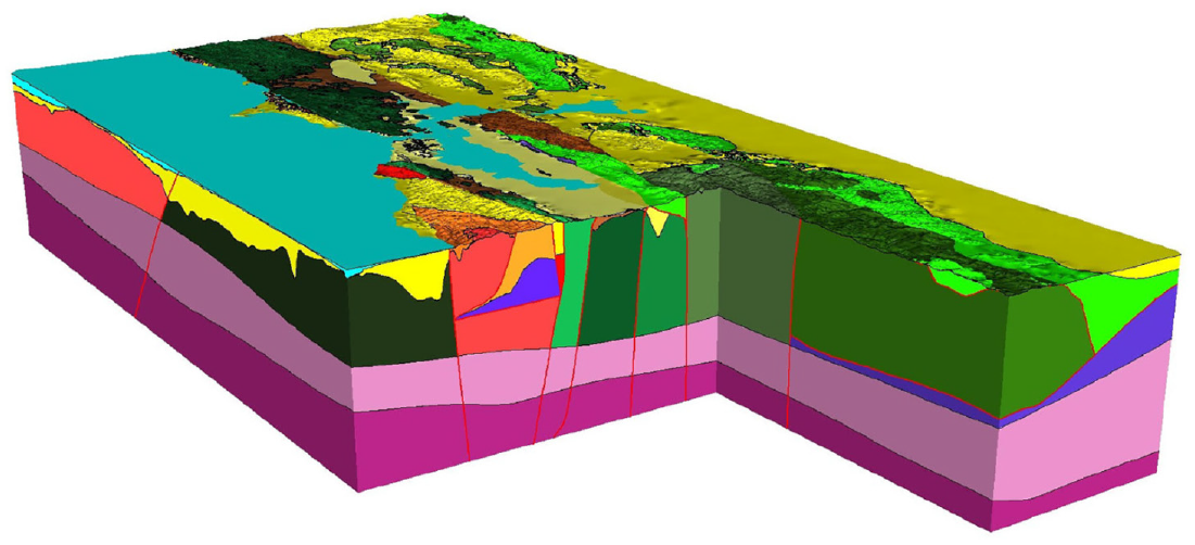
Conceptual and schematic 3D view of the San Francisco Bay Area geologic model (shared by Evan Hirakawa from the United States Geological Survey and available at https://www.usgs.gov/media/images/3d-geologic-model). The red lines display the main local faulting system in depth.
The velocity model performance was first evaluated through a qualitative comparison between recorded and simulated waveforms and then extended to a quantitative analysis. The overall modeling bias and its spatial variability were evaluated by comparing spectral amplitude residuals between recorded and simulated ground motions in the Fourier and spectral acceleration domains. The residuals’ spatial distribution allowed for the recognition of systematic suboptimal prediction patterns of under- or over-prediction extracted from direct comparisons between recorded and simulated data at a large number of seismic stations across the SFBA. We also used the waveform duration as another ground motion parameter to evaluate the performance of the velocity model. The comparison of the waveform duration between recorded and simulated ground motions aids us in identifying areas where the velocity model may not fully represent small-scale geologic features.
Several authors (e.g. Hu et al., 2022; Savran and Olsen, 2019; Taborda and Bielak, 2014; Taborda et al., 2016) have adopted the Anderson’s (2004) scale in quantitative evaluations of ground motion simulation performance. Anderson’s scale provides a quantitative framework to evaluate the match between recorded and simulated waveforms. Nevertheless, its applicability is limited beyond a relative comparison between scores from different studies. Other authors have used goodness-of-fit plots to analyze the waveform matching in the spectral response and Fourier domains (Hernández-Aguirre et al., 2023; Pitarka et al., 2004; Smerzini et al., 2022). In contrast, the methodology used in our study quantifies the epistemic uncertainty induced by the velocity model, allowing direct estimation of the misfit between simulated and recorded data. This misfit is expected to be inherent to any simulated wave field propagated through this velocity model. Therefore, we can directly propagate the estimated epistemic uncertainty in seismic hazard analysis applications.
This article starts by describing the earthquakes used in this study and our approach to modeling the seismic sources. Then, we present the key features of the USGS velocity model, characterized by blocks delineated by the local faulting system. Once the seismic sources and the velocity model are described, we evaluated the velocity model performance using the aforementioned intensity measures that quantify the accuracy of the simulated ground motions. Finally, we discuss our results regarding the performance of the USGS velocity model and the potential implications of our findings on constraining wave path effects in ground motion simulations for large earthquakes in the SFBA.
Seismic source characterization
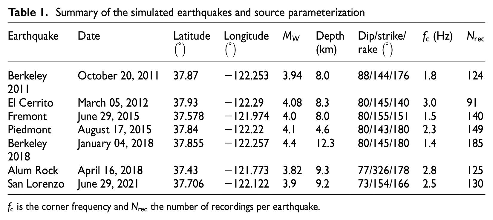
The seven small-magnitude earthquakes used in our simulations occurred between 2011 and 2021, with magnitudes ranging from 3.8 to 4.4. Six of the 7 events occurred on the Hayward fault, and one occurred on the Calaveras fault (Alum Rock event), close to the point of merging between these two faults. Simulating events on the western side of the San Francisco Bay would widen the azimuthal sampling. However, no events with magnitudes above 3.5 have occurred on the San Andreas fault in the last 20 years. Table 1 presents the location of each earthquake and Figure 2 shows a map of the earthquake epicenters, their focal mechanisms, and the stations used in our simulations.
Summary of the simulated earthquakes and source parameterization
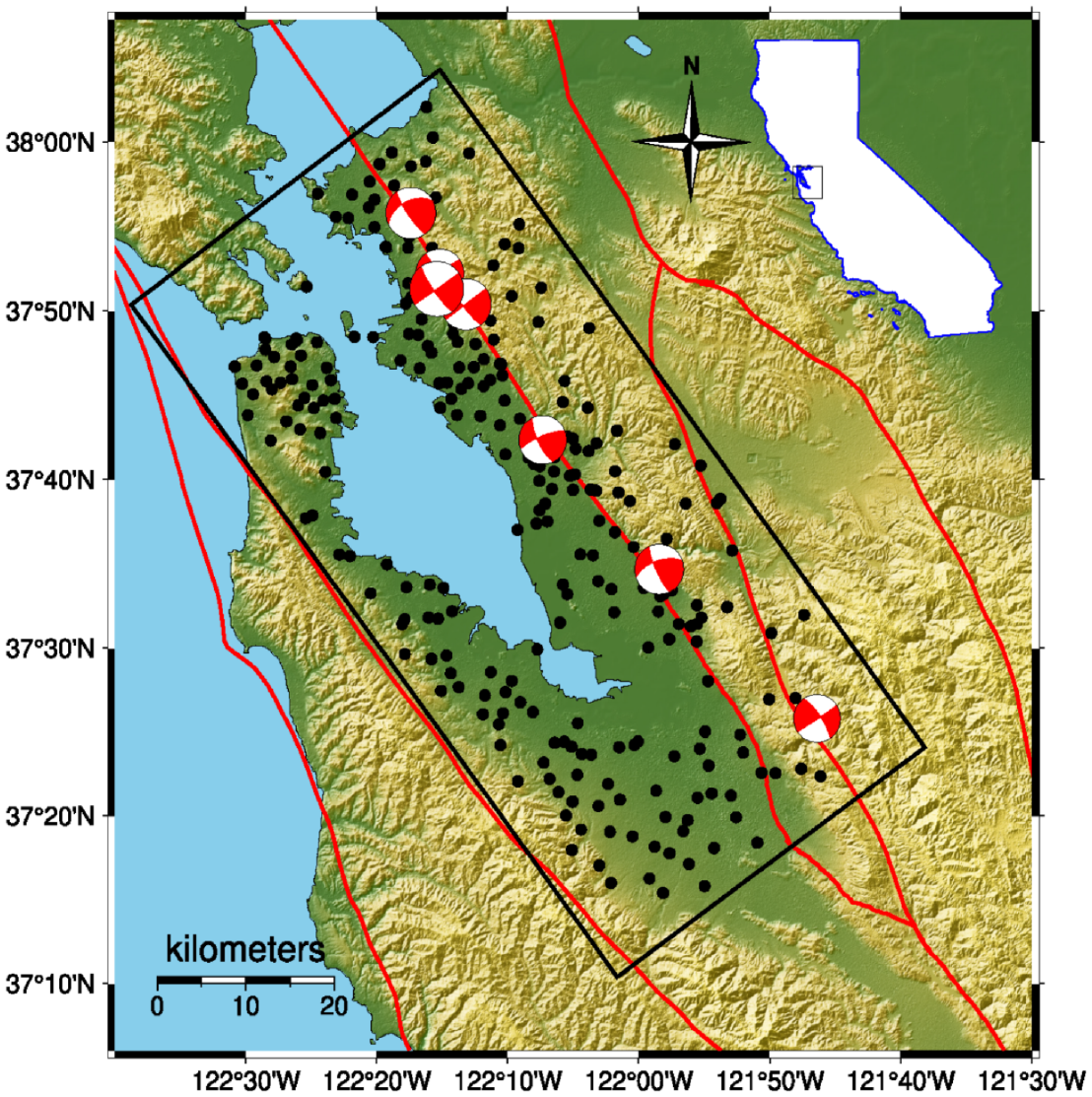
Map of the San Francisco Bay Area showing the locations of the stations (black dots), small earthquakes indicated by their focal mechanism, and the computational domain (black rectangle) used in this study. The red traces represent the regional fault system in the San Francisco Bay Area. The inset at the top-right corner shows the specific area of study with respect to the California state.
The earthquakes were simulated by double-couple point sources. The data from Hirakawa and Aagaard (2022) were adopted for the source and focal mechanism characterization (strike, dip, rake, depth, epicenter location, and magnitude), except for the San Lorenzo earthquake, which occurred after the publication of their article. Hence, its double-couple source mechanism was characterized using the information reported by the Northern California Earthquake Data Center. Table 1 presents the source parameters adopted in modeling the seven earthquakes.
The recorded waveforms were downloaded using the mass-downloading module from the open-source ObsPy package written in Python (Beyreuther et al., 2010). A small number of recordings were discarded as being unreliable based on inconsistencies in the timing of waveform phases. The dataset used in our study has a total of 943 records over 7 events and 273 stations. The simulated and recorded waveforms were resampled to 0.01 s, and a Butterworth acausal bandpass filter of order 3 between 0.1 and 5 Hz was applied. After transforming the waveforms to the Fourier domain for the Fourier amplitude analysis, we smoothed them using a Hanning window of 13 points.
The Liu source-time function (STF; Liu et al., 2006) was adopted to model how the source releases energy over time. Being consistent with rupture dynamics, this slip rate function is not symmetric; it is characterized by a large initial peak and a gradual amplitude decay that represents the healing process of the rupture (e.g. Pitarka et al., 2021).
The corner frequency,
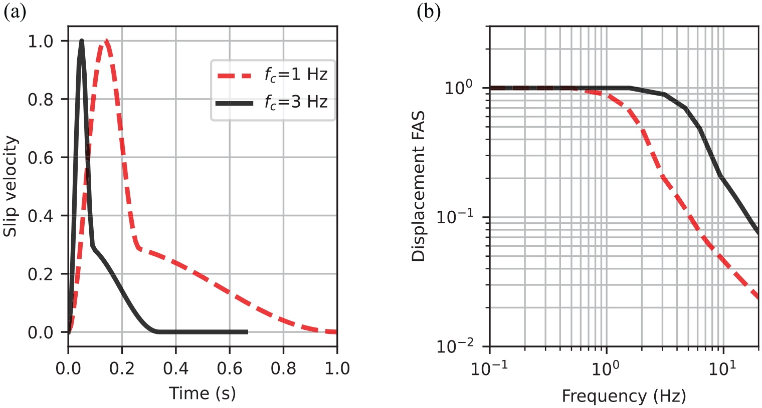
Example of Liu source-time functions for two corner frequencies: 1 and 3 Hz. (a) Slip velocity of the source-time function in the time domain. (b) Displacement spectra of the source-time function in the Fourier domain. The source-time function amplitude was normalized in the time and Fourier domain.
Velocity model
In our simulations, we used a sub-domain of the detailed USGS v21.1 SFBA VM (Aagaard and Hirakawa, 2021). This sub-domain includes the sedimentary basin and the hills on the east and west sides of the Bay Area. The free surface shear-wave velocity is shown in Figure 4. The Hayward fault causes an abrupt change in the materials’ seismic properties along most of the fault trace, which can be seen in the map view of the free surface shear-wave velocity. Toward the west of the Hayward fault, the surficial materials are softer, representing soft marine sediments and artificial fills. The eastern side of the Hayward fault has stiffer materials that have been uplifted by the local tectonic activity.
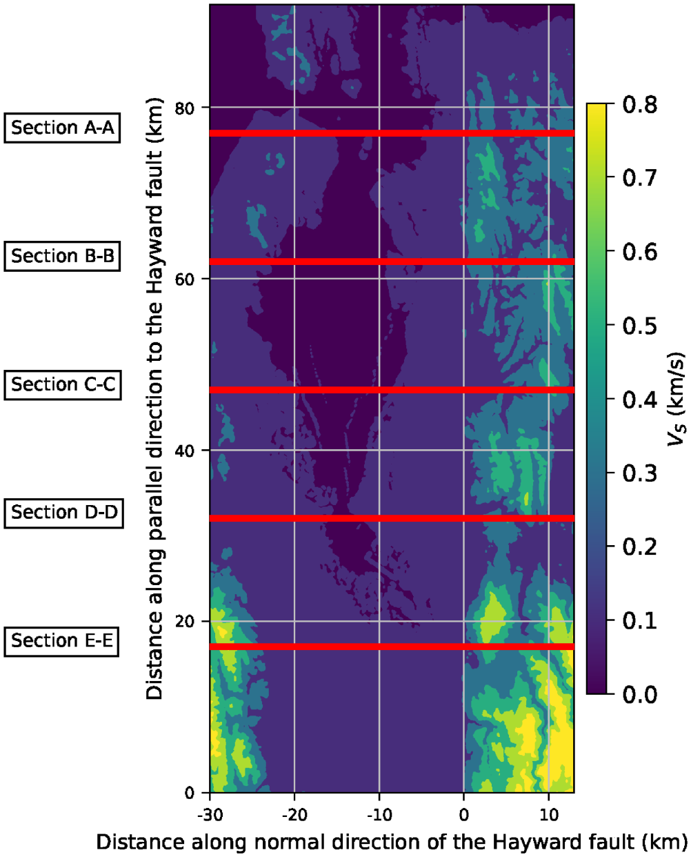
Map view of the free surface shear-wave velocity in the simulation domain, extracted from the United States Geological Survey velocity model. The thick E-W red lines indicate the location of the velocity model cross-sections shown in Figure 5.
The SFBA region has complex geological structures that are expected to have a significant effect on wave propagation across the Bay Area. The northern area is characterized by two blocks separated by the Hayward fault, as it is shown in the cross-sections A-A,B-B, and C-C in Figure 5. The block located west of the Hayward fault has a shallow layer of soft Quaternary marine sediments, underlaid by sedimentary basins that extend up to 1 km depth (see cross-sections B-B and C-C) and then by sequences of sandstones and sedimentary metamorphic rocks, the Franciscan complex (Bailey et al., 1964; Phelps et al., 2008). The eastern block is constituted mainly by sequences of sedimentary rocks deposited in the late Mesozoic Era, the Great Valley complex (Bartow and Nilsen, 1990). The shallowest layers in the eastern block are characterized by stiffer materials than those in the western block. Due to this geological contrast, the eastern block tends to be stiffer at the surface than the western block, with shear-wave velocities usually above 500 m/s, but at larger depths, it has lower shear-wave velocities than the western block.
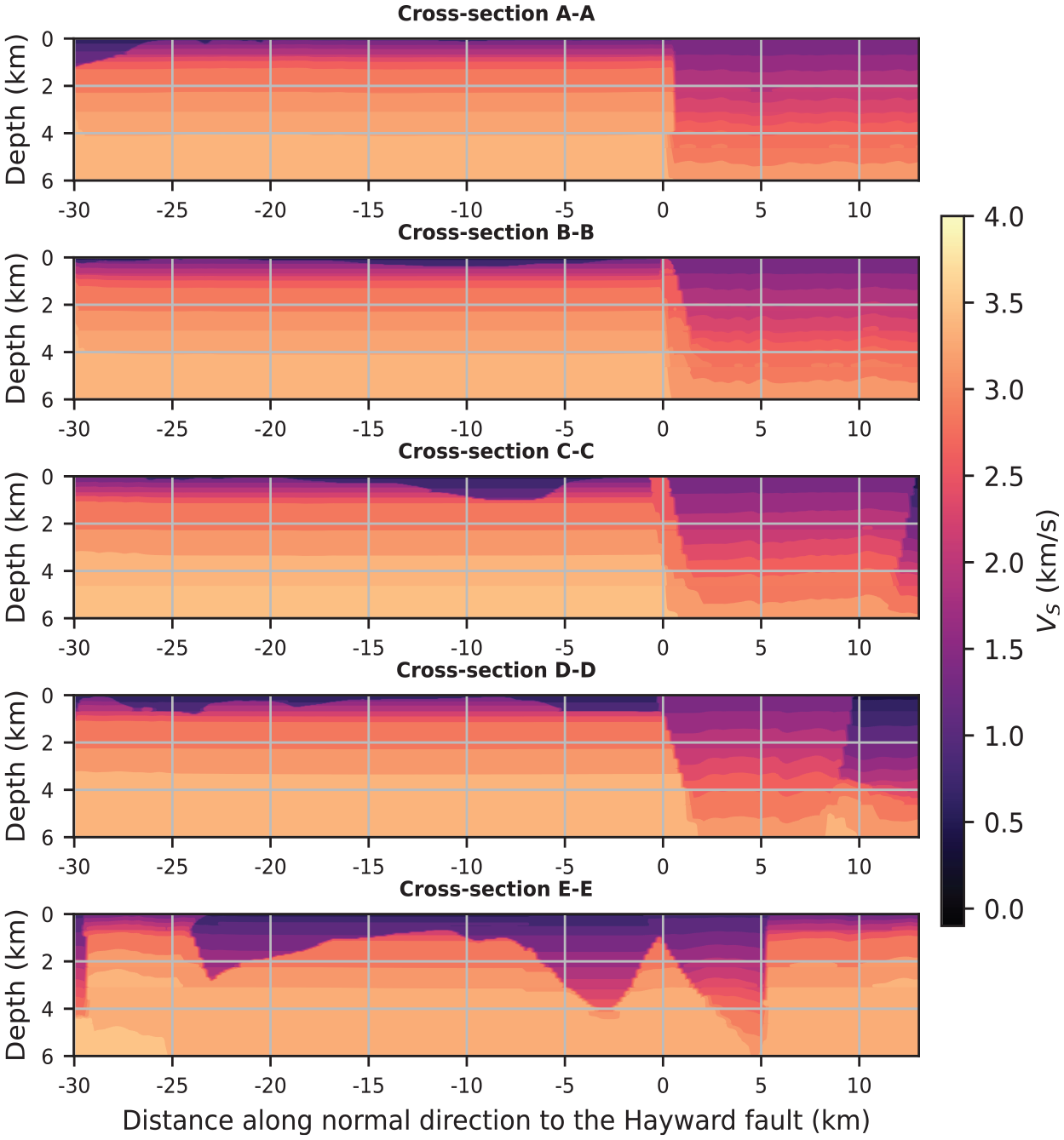
Northeast-southwest vertical cross-sections of the velocity model. The location of the cross-sections is indicated in Figure 4. The Hayward fault can be identified at 0 normal distance, through the strong velocity contrast between the western and eastern block. The Calaveras fault can be identified in cross-sections C-C and D-D as the dipping block around coordinate 10 km. Despite the simulations being run with topography, these cross-sections do not include the topography.
As shown in the cross-sections D-D and E-E in Figure 5, the local geology in the southern area of the western block is more complex than that in the northern area. The Calaveras fault bounds the eastern block from the east, shortening its width toward the south as seen in the cross-sections C-C, D-D, and E-E. The San Jose and Santa Clara regions, shown in the cross-section E-E, between horizontal coordinates −24 to 5 km, are underlaid by deeper sedimentary basin structures with an irregular geometry. The effects of these structures on the simulated waveforms are mostly manifested by basin wave reverberations and secondary surface waves that increase the waveform complexity and ground motion duration, as Frankel et al. (2001) showed by deploying a seismic array in the southern Bay Area.
In addition to the potential misrepresentation of the deep underground structure, another source of epistemic uncertainty in community velocity models is the simplification of the near-surface materials (e.g. Taborda and Bielak, 2014). The seismic properties of near-surface materials at shallow depths are usually represented by the time-averaged shear-wave velocity in the first 30 m,
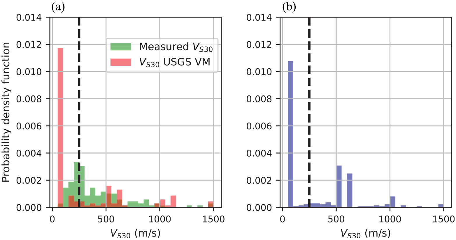
(a) United States Geological Survey velocity model-based (red bars) and measured (Tehrani et al., 2022; green bars)
Our ground motion simulations were performed with SW4, a parallelized computer program that employs an elastic finite difference method to solve the elastic wave equation in heterogeneous media. SW4 allows for the inclusion of a curvilinear mesh with vertical refinement to model the surface topography (Petersson and Sjögreen, 2023). Our simulations included the surface topography, which has a resolution of 100 m at the surface and a minimum shear-wave velocity of 250 m/s. A minimum grid spacing of 6.25 m was required to ensure proper numerical accuracy for frequencies up to 5 Hz, thus ensuring 8 points per wavelength in all our mesh. The wave attenuation is modeled through a linear visco-elastic model characterized by the quality factors (
Velocity model performance
Qualitative analysis
Our qualitative analysis of the velocity model performance in ground motion simulations of recorded earthquakes was focused on characterizing the waveform fit in terms of amplitude and wave phases by using three categories: good, fair, and poor. They were based on three criteria. The first criterion is the similarity of wave phases, the second is the amplitude match in the time and frequency domain, and the third criterion is the waveform and amplitude fit considering all three components of ground motions. A good waveform fit means that, overall, the recorded and simulated ground motions satisfy all three criteria. A fair fit means that at most two of the three criteria are satisfied. A poor fit is a case where two or more criteria are not satisfied.
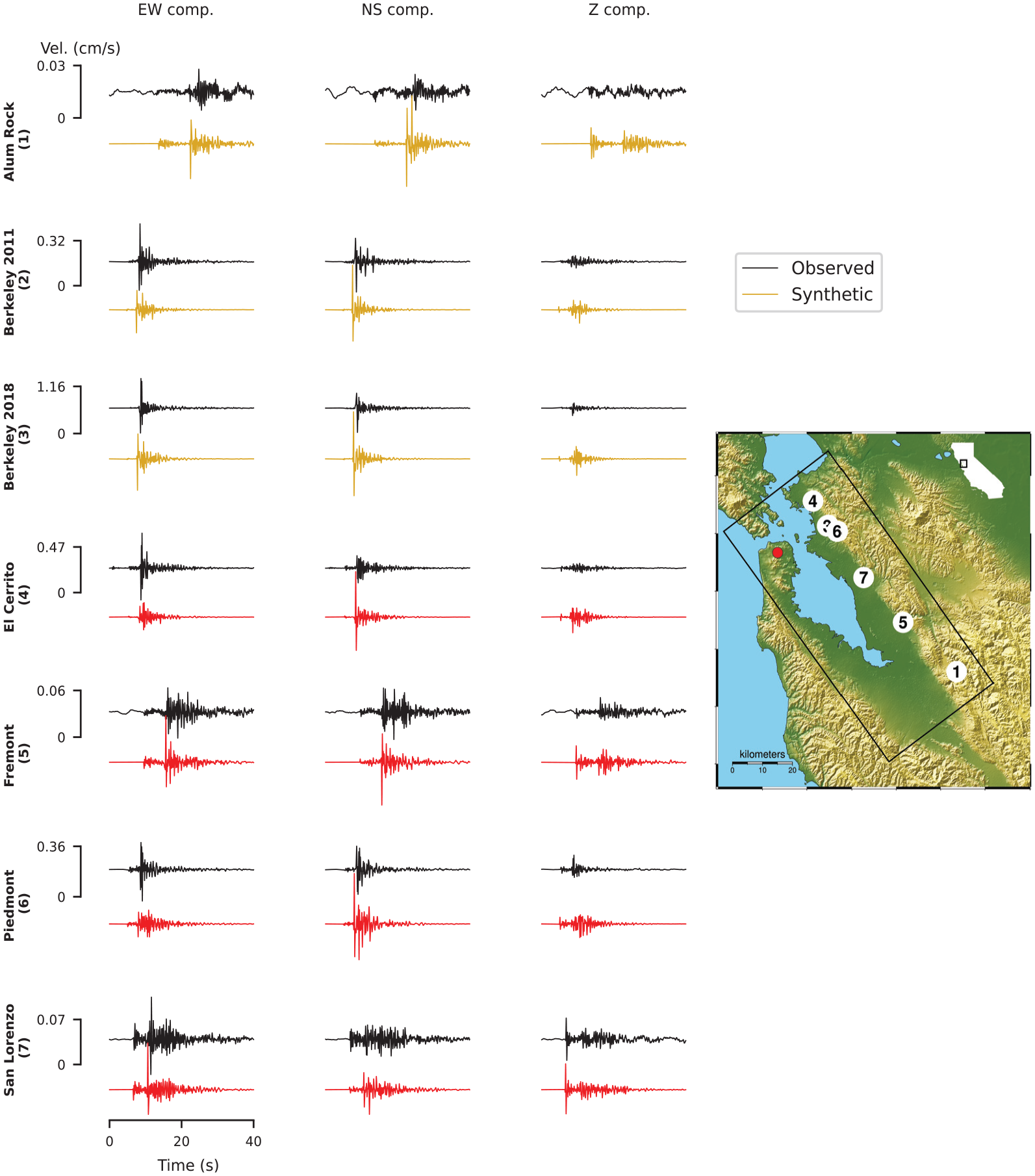
As illustrated in Figure 7, the quality of the simulated waveforms at a given station (J056) is event-dependent, implying a wave path dependency. The waveform fit at this station is good for four earthquakes and fair for the three others. This site is located on the San Francisco Peninsula, which, as shown later, is a region that manifests azimuthally dependent wave path effects, especially at high frequencies. Nevertheless, the simulated ground motions at this station capture most of the recorded waveform complexities associated with basin effects along wave paths crossing the San Francisco Bay. Figure 8 demonstrates that for a given seismic source, in this case the Berkeley 2018 earthquake, the waveform fit varies from good to poor depending on the station location relative to the seismic source. A similar trend is also seen in the frequency content of the waveforms, as shown in Figure 9, where we compare the recorded and simulated Fourier amplitude spectra of the waveforms shown in Figure 8.
Waveform match quality at station J056. Comparison of recorded (black) and simulated (different colors) waveforms of ground motion velocity for the seven earthquakes, band-passed filtered between 0.2 and 5 Hz. The earthquake’s name is indicated on the left of each trace. Red color indicates good, and yellow indicates fair waveform match quality. The amplitude for the plots was normalized within each earthquake, showing the maximum value between the six waveforms of each earthquake in the vertical axis.
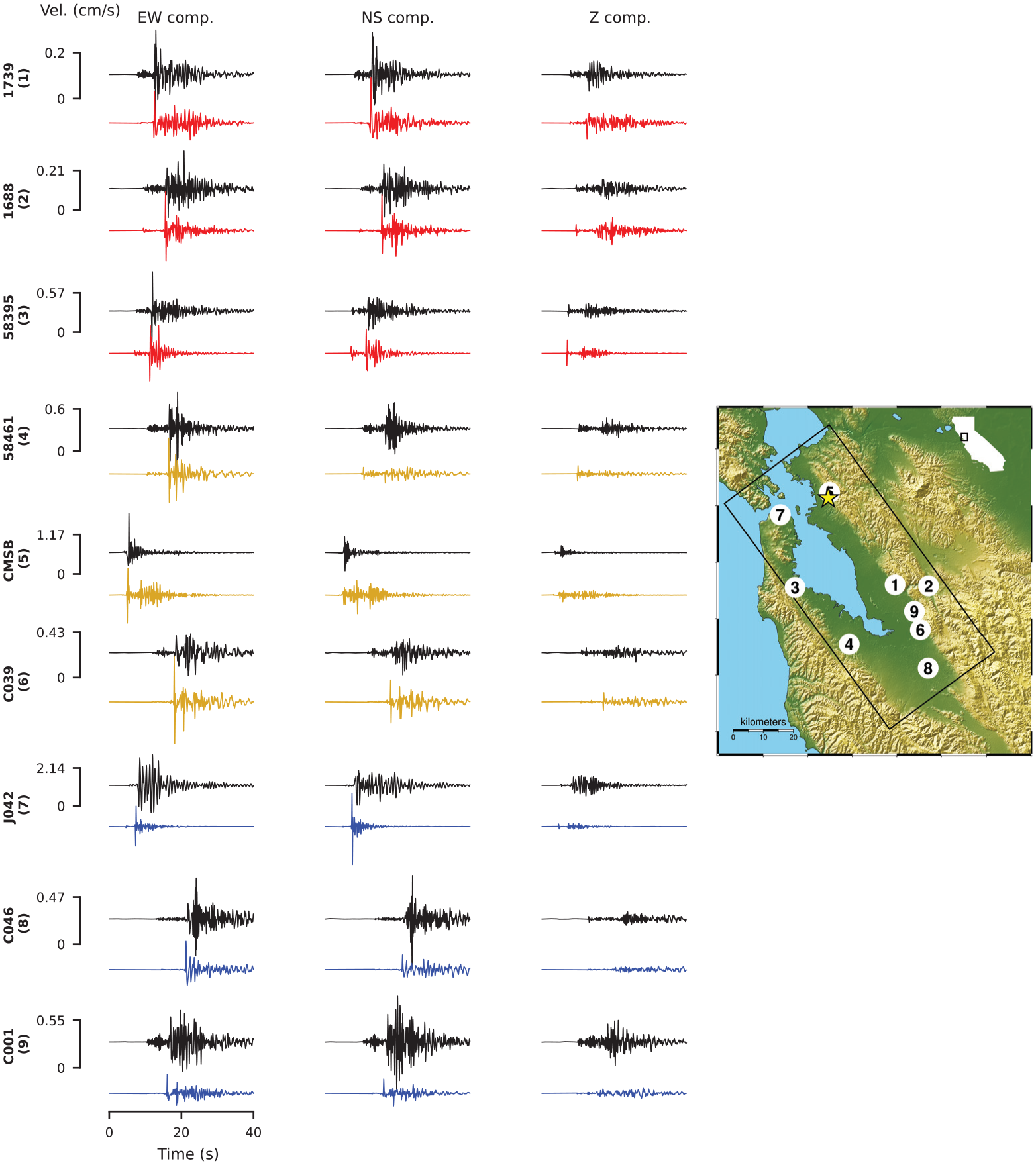
Comparison of recorded (black) and simulated (different colors) waveforms of ground motion velocity band-passed filtered between 0.2 and 5 Hz for the Berkeley 2018 earthquake at 9 stations. The station name is indicated on the left of each trace. Red, yellow, and blue colors correspond to good, fair, and poor waveform matching quality, respectively. The amplitude for the plots was normalized within each station, showing the maximum value between the six waveforms of each earthquake in the vertical axis.
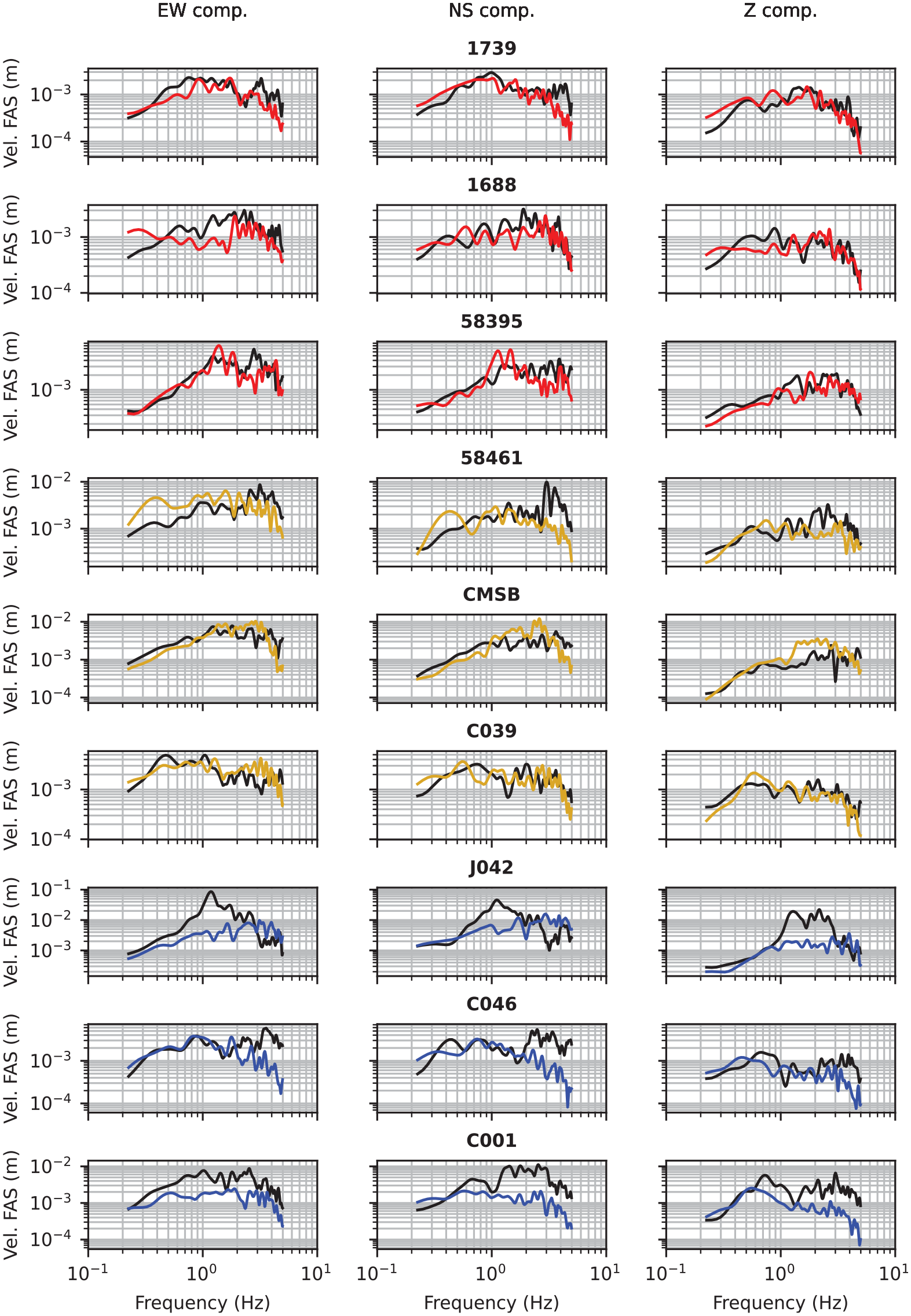
Comparisons of recorded (black) and simulated (different colors) Fourier amplitude spectra of ground motion for the Berkeley 2018 earthquake at the 9 stations shown in Figure 8. The station name is indicated above the central plot of each row. Red, yellow, and blue colors correspond to good, fair, and poor waveform matching quality, respectively.
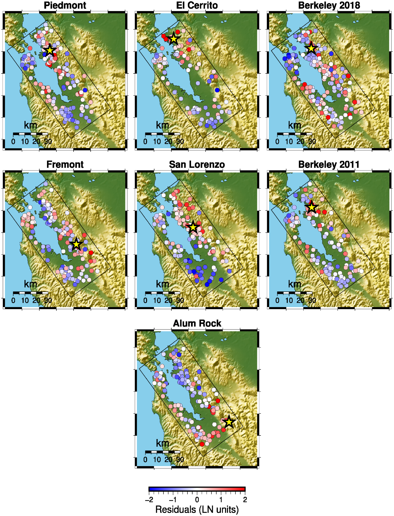
As a first-order comparison, the spatial pattern of the waveform matching can be used as an indicator of the quality of the velocity model along paths across the SFBA. This is demonstrated in Figure 10, which displays the simulated ground motion quality at all recording stations for all seven earthquakes. Although the overall spatial pattern of the simulated ground motion quality varies from one earthquake to the other, a close inspection reveals areas where the simulated ground motion quality is consistent among all scenarios. For example, the quality of the simulated waveforms is good at most of the stations located on the west edge of the bay, including some sites in the San Francisco Peninsula, for all the earthquakes. This demonstrates that the model is capable of reproducing wave propagation effects along paths across the bay. A similar observation can be made for most of the sites located on the east side of the bay, where the number of sites with good or fair quality waveform fit is much larger than those with a poor fit. It is important to note that the simplification of the source radiation pattern applied to the earthquake’s point source modeling can impact the simulation quality. The waveform quality at sites within the epicentral area and close to the nodal planes is sensitive to the focal mechanism, where a small misrepresentation of the focal mechanism can significantly affect the ground motion amplitude.
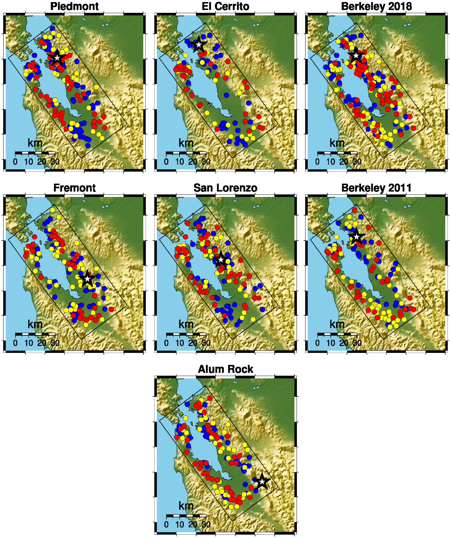
Waveform matching quality obtained for seven earthquakes at seismic stations indicated by colored circles. Red, yellow, and blue colors correspond to good, fair, and poor quality, respectively. The earthquake epicenter is indicated by the black star, and the earthquake’s name is indicated at the top of each panel.
Overall velocity model performance
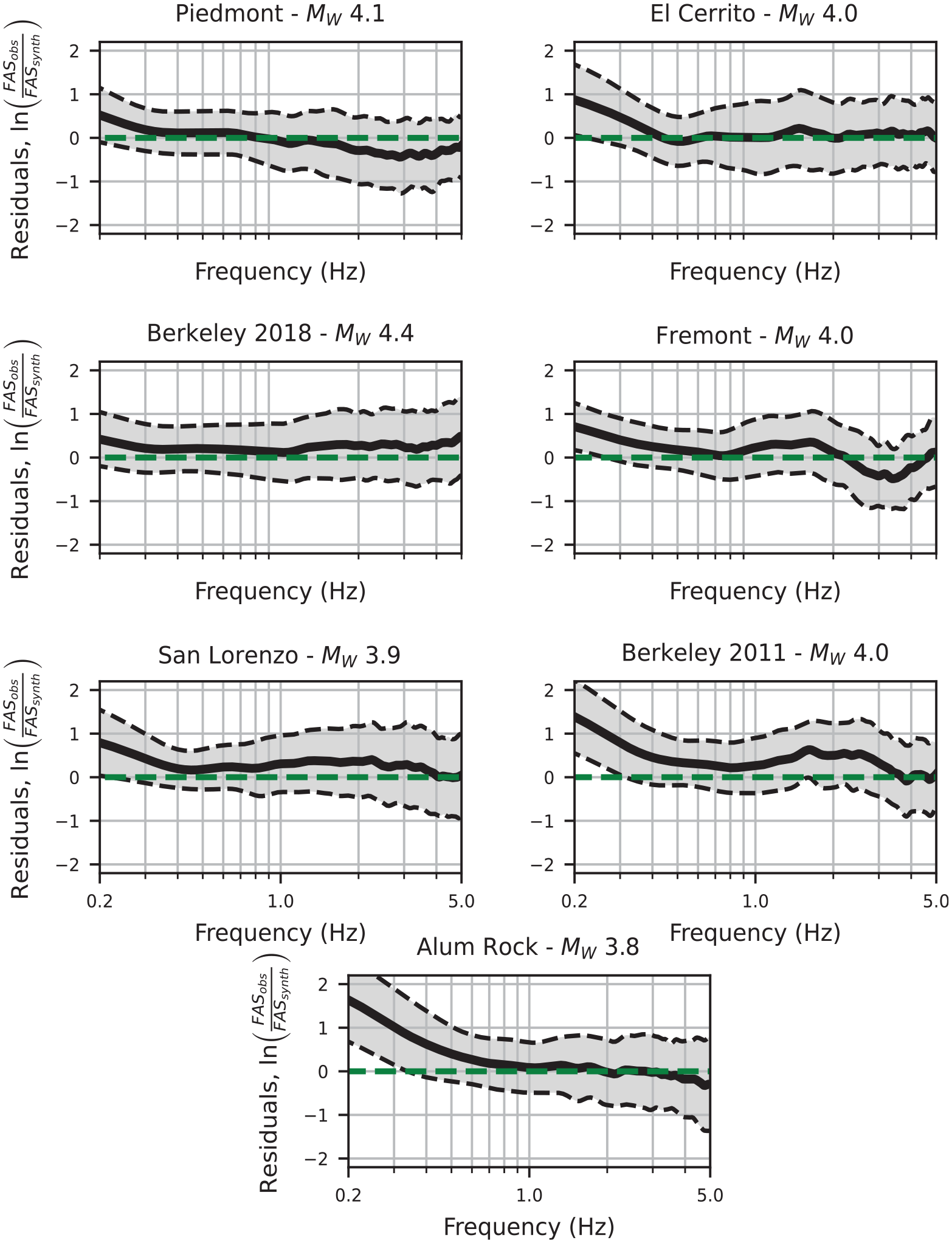
We evaluated the overall systematic bias between recorded and simulated data in the Fourier domain in the frequency range of 0–5 Hz to provide a quantitative assessment of the simulation performance. The Fourier amplitudes allow for a direct comparison of the frequency content of the recorded and simulated waveforms related to both source and wave propagation effects. The residuals between recorded and simulated waveforms in the log-natural scale are shown in Figure 11 for the horizontal component for each earthquake, adopting the format described in Goulet et al.’s (2015) study. Berkeley 2018, El Cerrito, and San Lorenzo show a near-zero bias between 0.2 and 5 Hz. The residuals of Piedmont, Fremont, Berkeley 2011, and Alum Rock fluctuate around zero, with a maximum over-prediction peak of 0.4 log-natural units (LN units) at frequencies above 3 Hz. The same comparison of residuals for the vertical component is shown in Figure 12. The vertical component shows mean residuals with larger between- and within-event fluctuations around zero; nevertheless, the maximum within-event bias does not exceed 0.5 LN units. Some events show a break point in the mean residual at low frequencies, with a trend toward under-prediction in the bias (positive bias), as for example Alum Rock with a bias of 1 and 1.5 LN units for the horizontal and vertical components, respectively. This mismatch is significant also for the El Cerrito, San Lorenzo, and Berkeley 2011 earthquakes. Because this mismatch is earthquake-dependent and is more pronounced at long-distance stations where the source-related long-period waves have relatively low amplitudes, our interpretation is that it is due to large-amplitude long-period ambient noise at the time when these three earthquakes occurred. This earthquake-dependent mismatch has also an impact in the standard deviation, which tends to increase below 0.4 Hz.
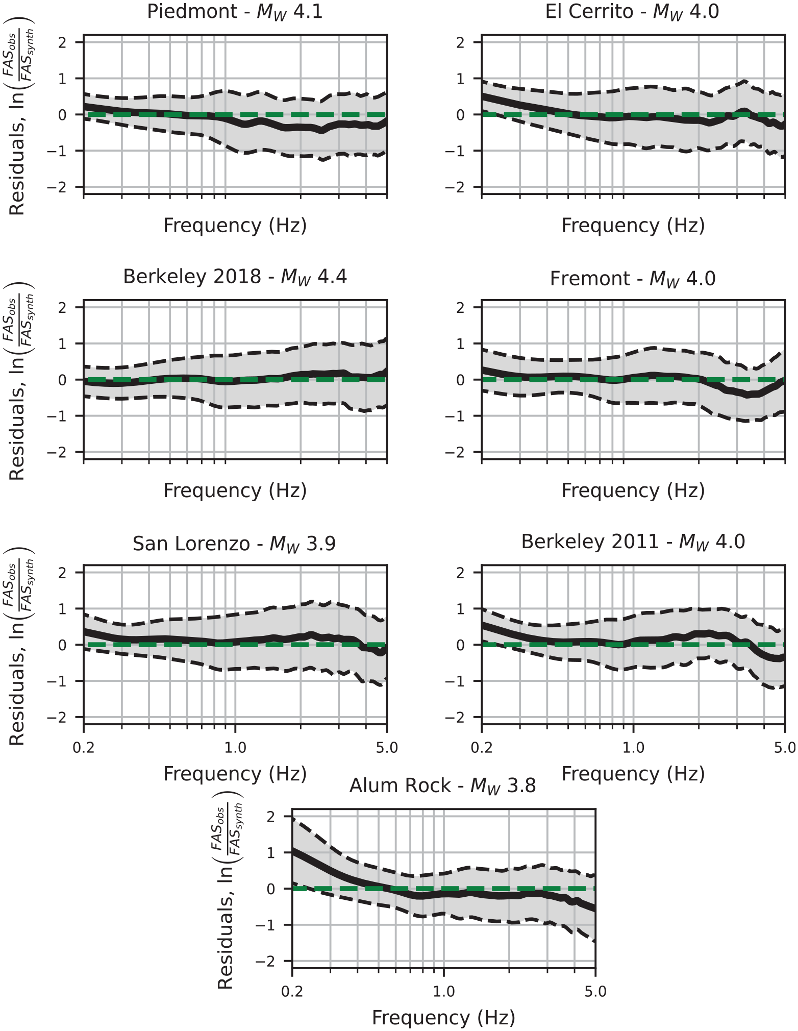
Comparison of the within-event Fourier amplitude residuals for the horizontal component of the ground motion averaged over the recording stations for each event. The solid line is the bias expressed by the log-natural of the amplitude ratio between the recorded and simulated motions as a function of frequency. The shaded area corresponds to the 16th–84th residuals’ percentile. Each panel corresponds to each of the seven earthquakes. The name of the earthquake is indicated on top of each panel.
Same as Figure 11, but for the vertical component.
It is important to note that, as shown in Figure 13, the simulations of the horizontal ground motion, when averaged across all seven earthquakes, have a near zero bias up to 3 Hz. This figure shows the mean and standard deviation of the horizontal and vertical components for the seven simulated earthquakes. The vertical component’s mean bias is centered at zero except for a frequency band between 1 and 3 Hz, where a slight under-prediction of around 0.25 LN units appears. We believe that the mismatch between the recorded and simulated ground motion at frequencies below 0.5 Hz, observed in almost all considered earthquakes, is caused by the relatively high local ambient noise.
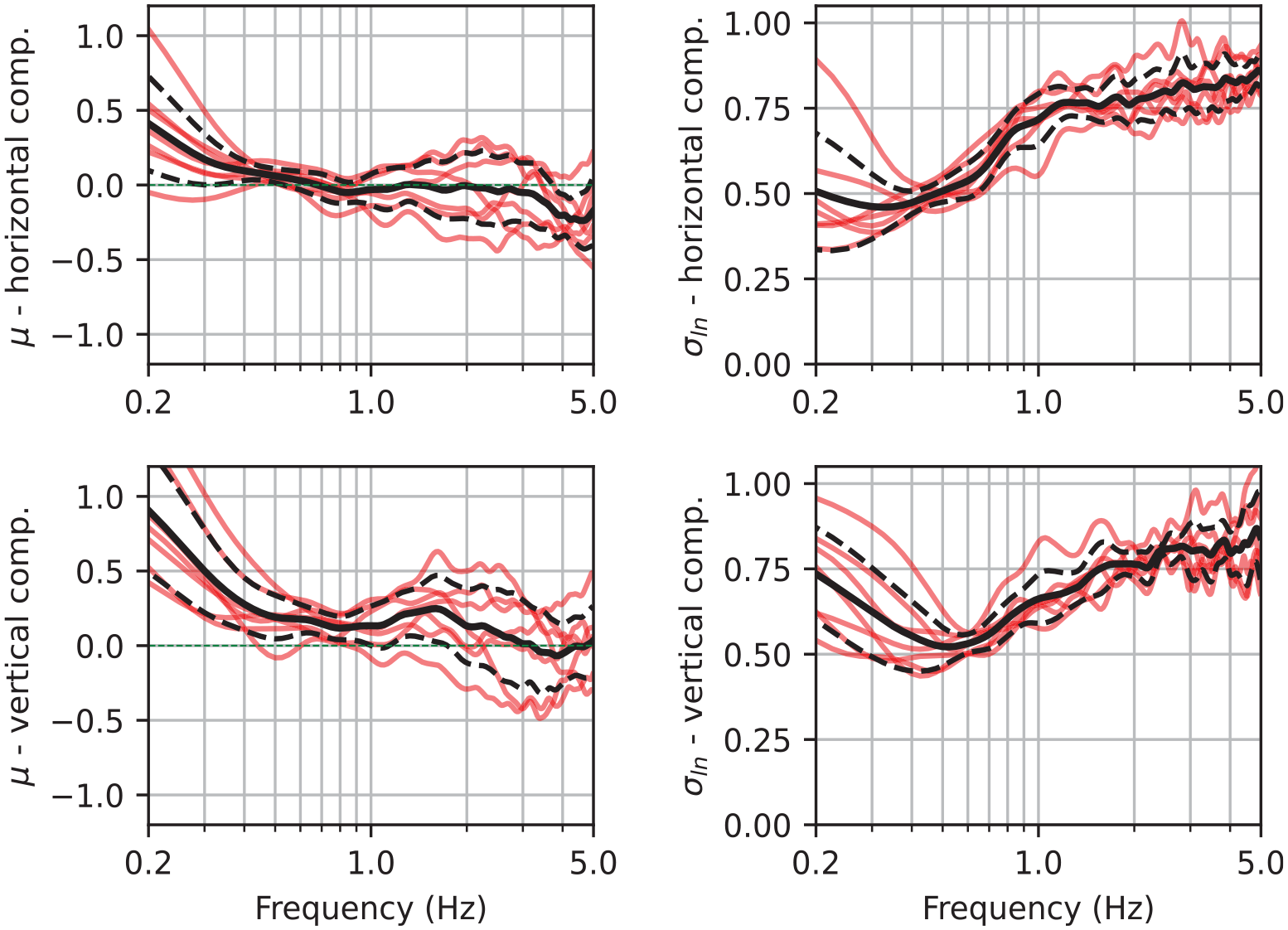
Mean (left panels) and standard deviation (right panels) of the within-event Fourier amplitude residuals averaged over seven simulated earthquakes. The upper and lower panels correspond to the horizontal and vertical components, respectively. The black solid lines are the mean of the 7 events, and the dashed lines correspond to the 16th–84th percentile. The red traces show the individual standard deviations for each earthquake.
The standard deviation of both components increases at higher frequencies, reflecting the impact of the mismatch between recorded and simulated ground motion due to small-scale heterogeneities, especially near the free surface (Lu and Ben-Zion, 2022). This behavior was also observed by Taborda et al. (2016) in their broadband simulations of the Chino-Hills earthquake in the Los Angeles basin using a 3D regional velocity model. They showed that the standard deviation between the recorded and simulated ground motions increases at higher frequencies. Another interesting finding in our analysis is that the standard deviation of the residuals is similar among all considered earthquakes, especially for the vertical component; the within-event standard deviation converges to a narrow band among the simulation of the 7 events. This implies that the accuracy obtained in our simulations and modeling methodology is stable among the 7 events.
Spatial distribution of spectral acceleration residuals
In this section, we analyze the spatial distribution of the spectral acceleration residuals. Maps of the spectral acceleration residuals for the horizontal component at 0.5, 1.0, and 4.0 Hz (2.0, 1.0, and 0.25 s) are illustrated in Figures 14 to 16, respectively. These maps show clear patterns of under- and over-predictions within each event at three different spectral frequencies. For example, a roughly circular region surrounding the San Lorenzo earthquake epicenter shows consistent patterns of under-prediction. On the other hand, the southernmost corner of our domain consistently displays over-predictions, suggesting that the soft sediments in the southwestern part of the SFBA can be singled out as areas where the model needs to be improved.
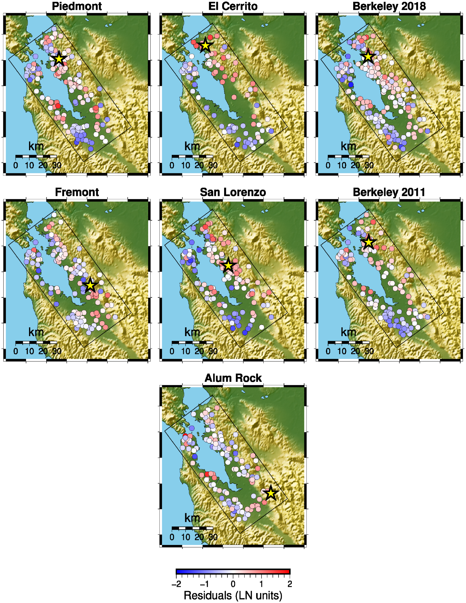
Total spectral acceleration residuals at 0.5 Hz computed at each station indicated by colored circles. The colored circles represent the residual and the yellow star the epicenter location.
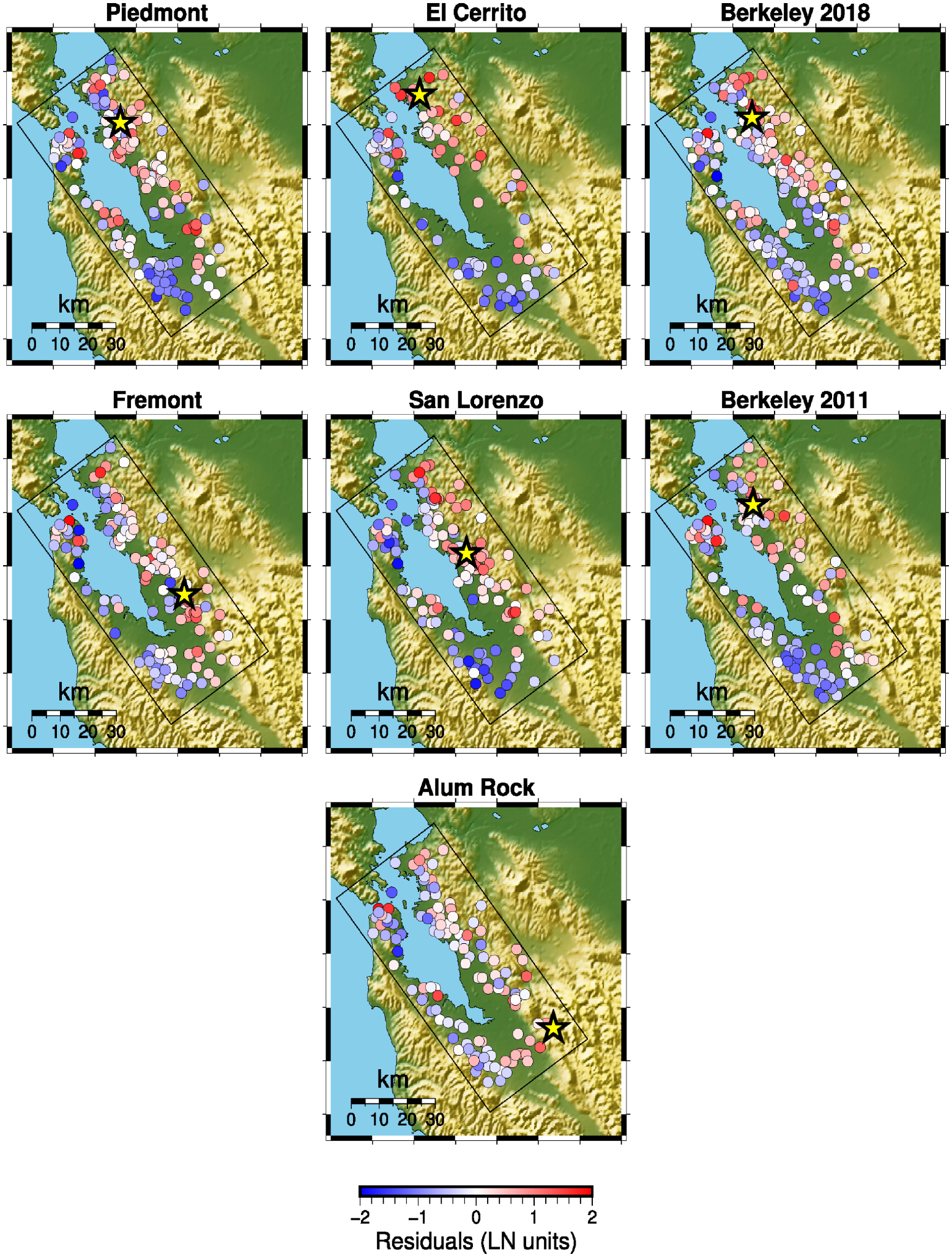
Total spectral acceleration residuals at 1.0 Hz computed at each station indicated by colored circles. The colored circles represent the residual and the yellow star the epicenter location.
Total spectral acceleration residuals at 4.0 Hz computed at each station indicated by colored circles. The colored circles represent the residual and the yellow star the epicenter location.
The spatial correlation of the residuals is a manifestation of poorly characterized path effects. For example, the West San Jose area (southwest corner of the San Francisco basin) exhibits strong path effects for different earthquakes at these three frequencies. The simulation of the San Lorenzo earthquake produces the largest over-prediction in this area, with a source site azimuthal variation between 150° and 180°. In contrast, the simulation of the Alum Rock earthquake produces the largest under-prediction with azimuths varying between 215° and 270°. This is consistent with Stidham et al. (1999) and Dolenc and Dreger (2005), who using 3D physics-based ground motion simulations and seismic array analysis, respectively, found strong basin effects in this region of the SFBA. The San Francisco Peninsula also experiences azimuth-dependent path effects. They are observed mostly at high frequencies. Ground motions of events located to the east of the basin are over-predicted at frequencies above 4 Hz (e.g. San Lorenzo and Fremont earthquakes), and for events located to the south, along the Hayward fault, the over-prediction gradually becomes relatively small (e.g. Alum Rock earthquake), and we can even observe a slight under-prediction of the ground motion amplitude. It appears at high frequencies, suggesting shallow geologic structures may cause this ground motion azimuthal variability.
To get a deeper insight into these 3D path effects, in Figure 17 we show the example of waveforms recorded and simulated at station 1796 in Santa Clara for the seven earthquakes. The recorded waveforms from earthquakes coming from the north to northwest exhibit phases with comparable amplitudes after the main shear-wave phase arrivals. In contrast, the waveforms coming from the northeast to the east (Alum Rock and Fremont) induce a smaller waveform reverberation in the recorded waveforms. The simulated data captured some of these phases after the main shear wave arrival but lacked the recorded waveforms’ complexities and amplitudes. This effect can also be observed in the simulated Fourier amplitude spectra (Figure 18). The shape of the simulated spectra from several events tends to be similar, while the recorded spectral shapes show more complex event-dependent variations, as relative spectral amplitude fluctuations between the recorded and simulated waveforms at a fixed frequency for different source–receiver pairs exist. The amplitude of the recorded waveforms at a given frequency is larger than the simulated waveforms for some earthquakes, while the opposite behavior is observed for others. A better representation in the velocity model of the 3D structures that induce these complexities is necessary for reproducing these recorded path effects.
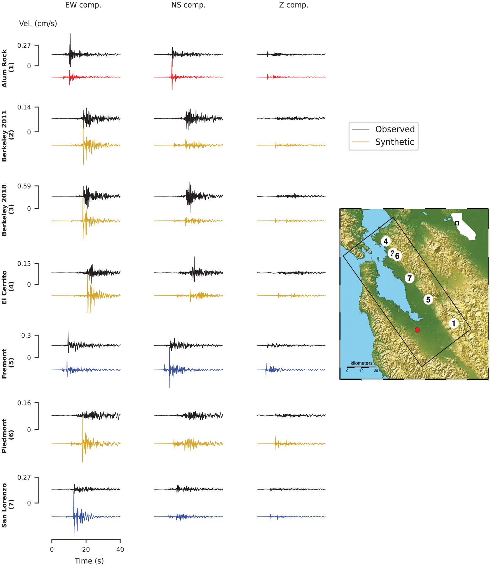
Comparison of recorded (black) and simulated (different colors) time histories of ground motion velocity band-passed filtered between 0.2 and 5 Hz at station 1796 (red circle in the map) obtained for the seven earthquakes. The earthquake name is indicated on the left of each trace. Red, yellow, and blue colors correspond to good, fair, and poor waveform matching quality, respectively. Numbered white circles in the map indicate the earthquake’s epicenter location. The amplitude for the plots was normalized within each earthquake, showing the maximum value between the six waveforms of each earthquake in the vertical axis.
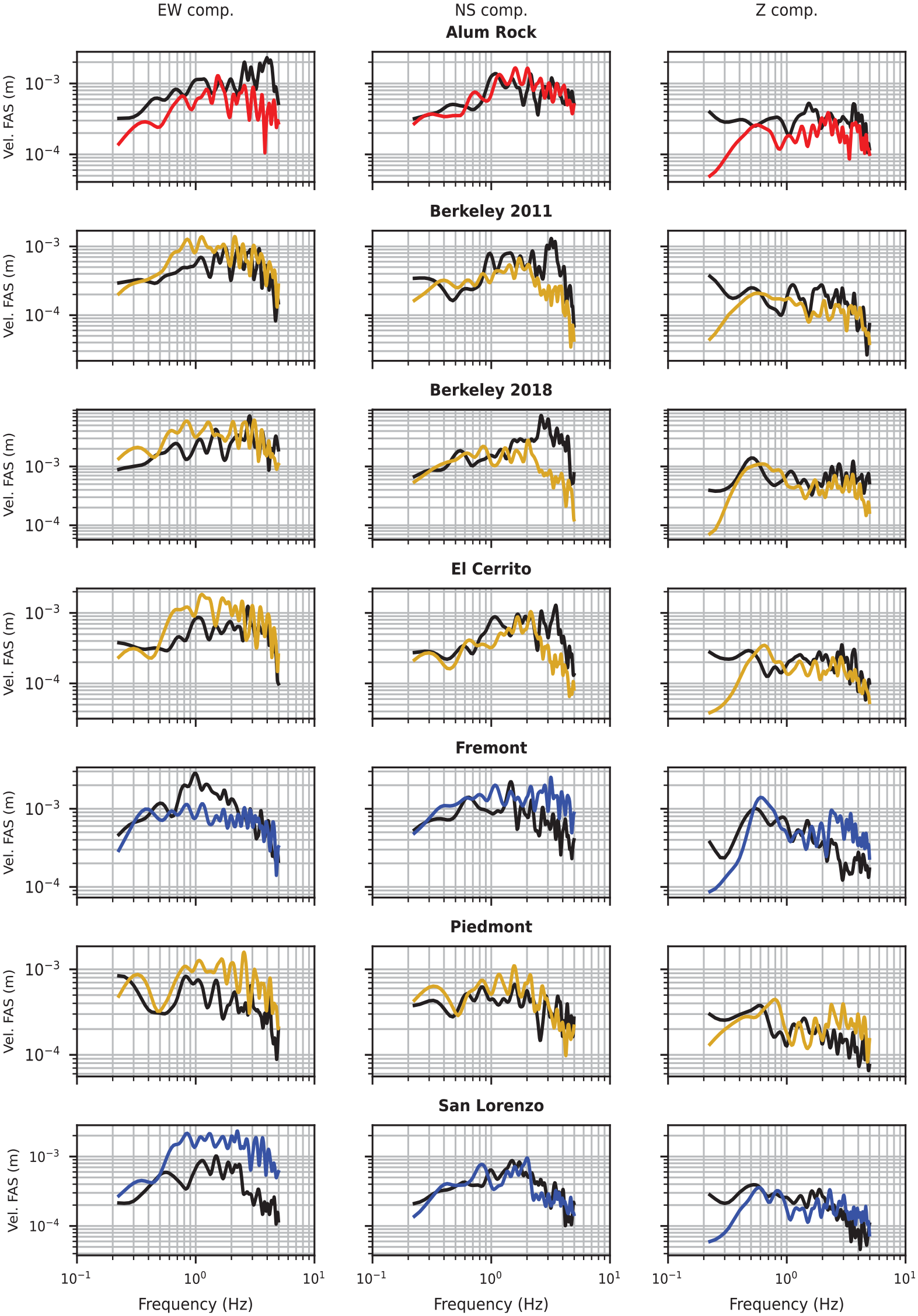
Comparisons of recorded (black) and simulated (different colors) Fourier amplitude spectra of ground motion at station 1796 obtained for seven earthquakes. The earthquake name is indicated on top of each panel. Red, yellow, and blue colors correspond to good, fair, and poor waveform matching quality, respectively.
The difference in the residual distributions obtained for the Piedmont and Berkeley 2018 and 2011 earthquakes indicates that earthquakes in similar locations but with different hypocentral depths can result in different wave propagation effects. This interesting observation can be made by analyzing the residual distribution from the previous maps and Figures 17 and 18, showing that the path effects are not only azimuthally dependent but also event-depth dependent. The close proximity of their epicenter could lead to the assumption that their impulsive response should be similar. However, the difference in their hypocentral depths (ranging from 4.5 to 12.3 km) impacts the wave fields, showing poorly represented depth-dependent path effects.
Modeling of spatial patterns of suboptimal predictions
One of the valuable features of this extensive database of small event observations is the opportunity to assess areas for potential improvement in the existing regional velocity model. The spectral acceleration residuals between recorded and simulated ground motions are spatially correlated, which allows us to model their spatial patterns. We estimate the median spatial distribution of these residuals to evaluate suboptimal prediction patterns in our computational domain (i.e. areas of systematic under- or over-prediction). We decoupled the residuals from the observation at site “s” from the earthquake “e” into three main terms as:

in which
Equation 1 was solved using the Gaussian process module of pymc, a Bayesian modeling package written in Python (Salvatier et al., 2016).
Inference of the spatially varying term,
Treasure and Yerba Buena islands are not characterized in the velocity model, keeping the same velocity structure as the nearby bay sediments (see Figure 4). The impact of this characterization is shown in Figure 19 with systematic patterns of over-prediction. The velocity model should be updated in this area by including the buried geology structures surrounding these islands, which give rise to the Yerba Buena outcrop.
The USGS velocity model performance will improve by explaining the sources of the discrepancies captured by
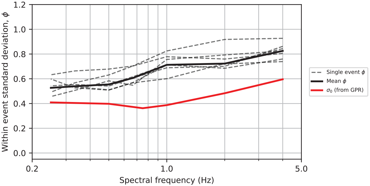
Within-event standard deviation for the spectral acceleration,
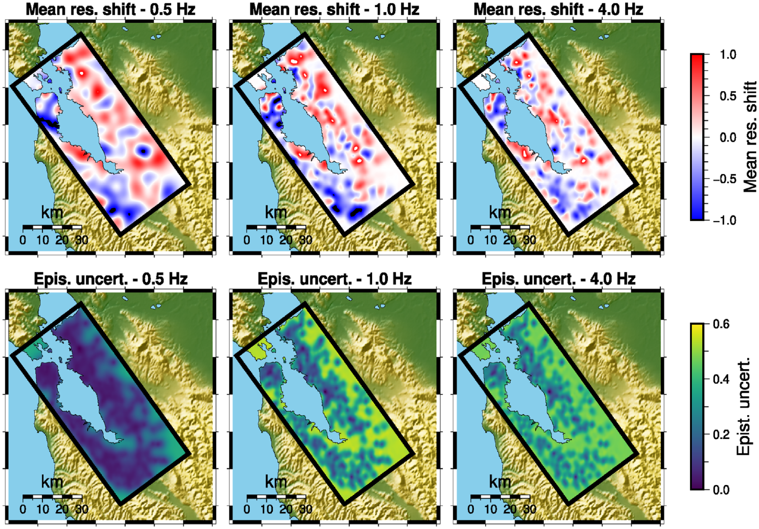
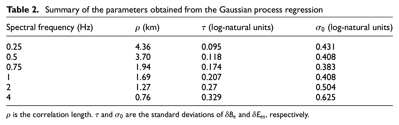
The hyper-parameters from the Gaussian process regression are shown in Table 2. The correlation length ranges from 4.36 km at 0.25 Hz to 0.76 km at 4 Hz, showing that the higher the frequency, the smaller the correlation length. The standard deviation of
Summary of the parameters obtained from the Gaussian process regression
The spatially varying systematic misfit,
Waveform duration analysis
Complex geologic structures cause wave scattering, which can create secondary wave phases in addition to primary source-generated body waves and surface waves. Most of these phases, also known as coda waves, arrive after the primary shear waves, thus increasing the duration of ground motions. The normalized Arias intensity is often used to quantify how the total seismic energy is spread over time, indirectly quantifying the presence of these additional phases (Pinilla-Ramos et al., 2023). We adopt
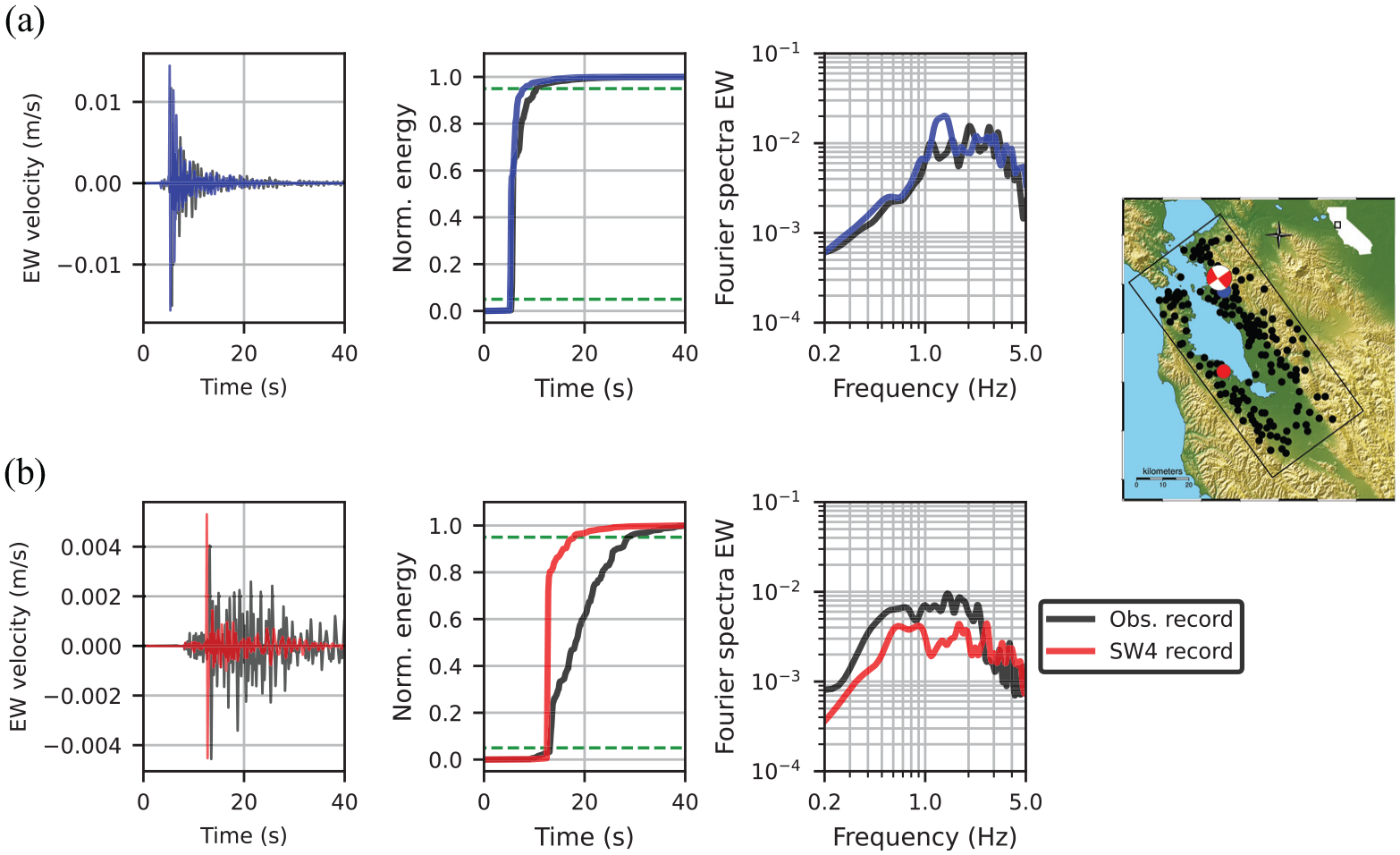
Example of waveforms’ duration at two sites for East-West (EW) component. (a) Station C005 (blue color) shows a similar duration between simulated and recorded waveforms. (b) Station J037 (red color) develops strong surface wave amplitude in the recorded waveforms after the arrival of the shear-wave phases. The simulated waveforms do not develop this more complex impulsive response pattern.
We evaluated spatial patterns of
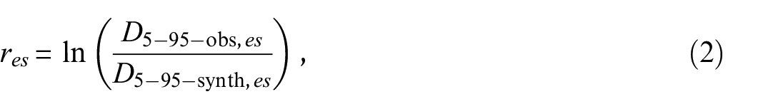
in which
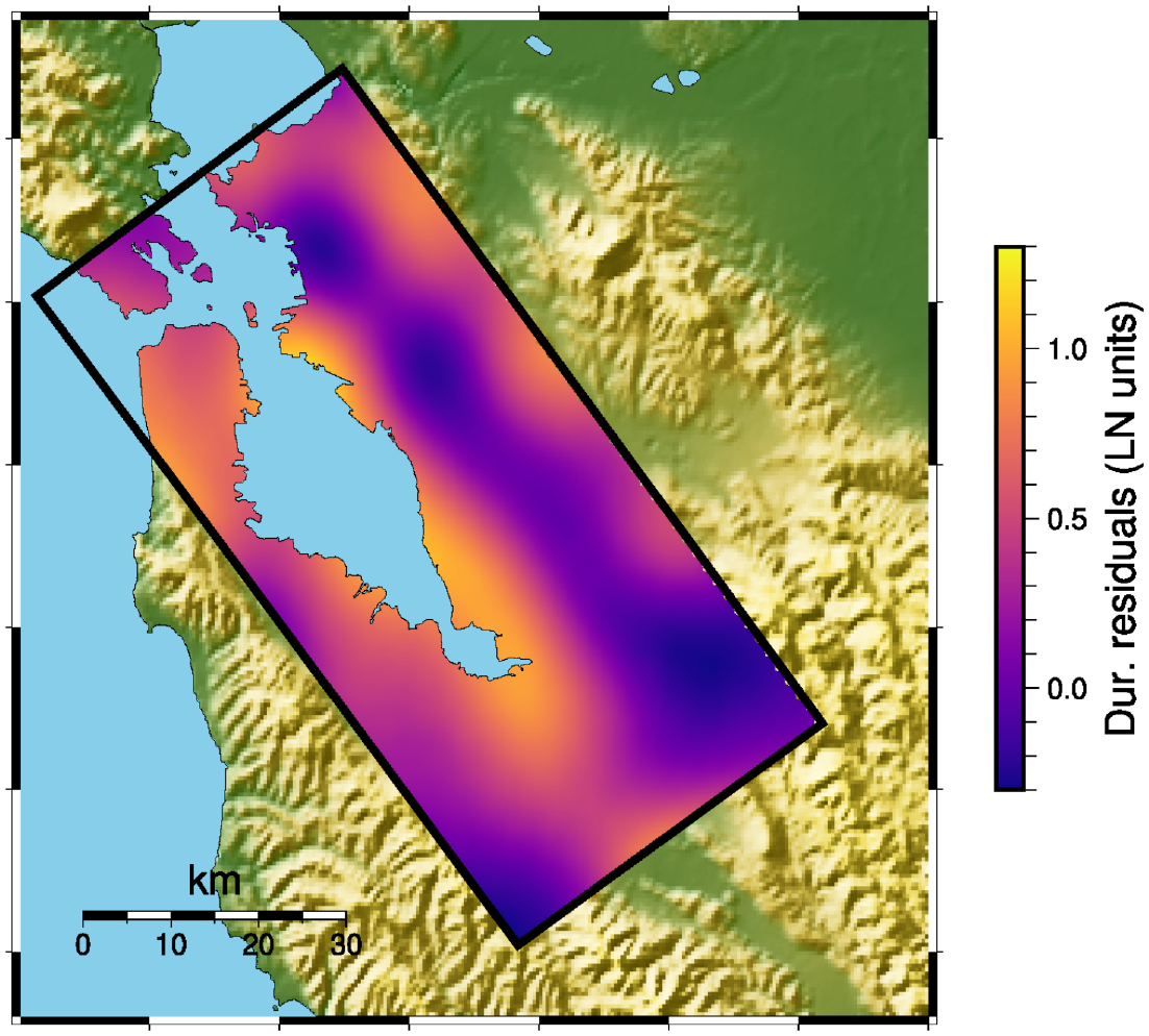
Spatial distribution of the
Discussion
This study focuses on the performance evaluation of the USGS velocity model using physics-based ground motion modeling of earthquakes in the SFBA. In our analysis, we tried to identify the cause of the misfit between the recorded and simulated ground motions, which can mainly be linked to the velocity model, earthquake source, and material stress–strain characterizations adopted in our simulations. Conceptually, we can decouple the variance of the systemic misfit between simulated and recorded waveforms as:

in which
Use of spatial patterns of suboptimal predictions to improve the velocity model
The spectral amplitude residuals’ maps identify features that can be enhanced in future versions of the velocity model, quantifying the benefits of these improvements. For instance, the soft sediments of the Bay basin tend to produce systematic over-prediction of the recorded ground motion, suggesting that the model needs improvements in areas with very soft surface sediments. Moreover, the western block exhibits over-prediction of spectral acceleration, especially in Santa Clara, San Jose, Fremont, and several areas of the SFBA. This could also be due to differences in the actual shallow velocity structure, but this time with the velocity model having lower values. In addition, the seismic properties in the regions surrounding Treasure Island and Yerba Buena Island, where the current USGS velocity model does not include the rock outcrop of these islands, need to be added.
We modeled the residuals using Gaussian process regressions, a stochastic machine learning technique (Rasmussen and Williams, 2005) that allows us to track these spatial patterns. By explaining the sources of the differences our model identified, being tracked by
Future refinements of the velocity model can take advantage of the fact that in California,
Corner frequency
The corner frequency,
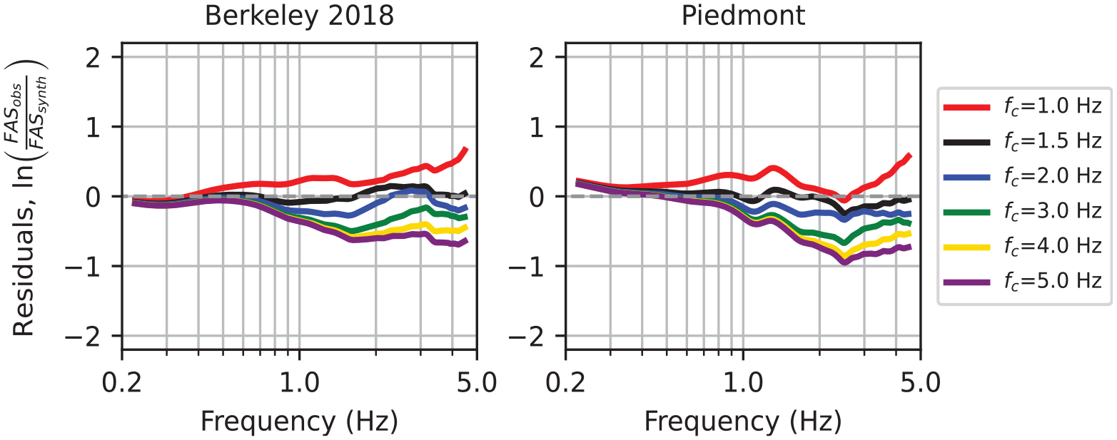
Sensitivity analysis performed on the corner frequency,
Earthquake location
As was shown in the “Velocity model” section, there is a strong impedance contrast between the western and the eastern block of the Hayward fault. Because of this lateral contrast, the wave field has multiple paths compared to a 1D velocity model (Baise et al., 2003; Stidham et al., 1999). Head waves traveling through an interface with strong impedance contrasts will arrive earlier in the softer block (Allam et al., 2012) compared to a 1D velocity model, which, together with the manifestation of multiple paths, add complexities to the estimation of the event location. Nevertheless, the waveform comparison between recorded and simulated data does not show a significant bias in the arrival time, meaning that, on average, the sources’ locations and the velocity model adopted provide good results. This indicates that the added complexities to the estimation of the event location have little effect in this case. This is consistent with Hirakawa and Aagaard (2022), who updated this version of the velocity model based on inversions of the arrival time of waveforms from small-magnitude earthquakes through simulations using SW4.
Stochastic variability in the velocity model
We showed that the velocity model has an overall good performance, with a slight systematic over-prediction at high frequencies (above 3 Hz) and a shorter duration of the simulated waveforms compared to the recorded waveforms. One possibility for improving the performance at high frequencies is the inclusion of stochastic variability in the velocity model. This leads to more realistic waveforms (Savran and Olsen, 2019; Pitarka and Mellors, 2021), being able to reconcile this bias observed above 3 Hz and improving the waveform matching (Graves and Pitarka, 2016). Adding stochastic variability in the geologic structure will aid in reconciling some differences observed in the waveform duration by adding more phases induced by internal reflection effects due to a more diffuse wave propagation regime. Natural materials have inherent variabilities in their properties spread out in space, and data are needed to constrain the stochastic perturbation generator models. Consequently, the inclusion of stochastic small-scale variability in velocity models is expected to improve the quality of the simulated ground motion on a broad frequency range (e.g. Graves and Pitarka, 2016). Despite the fact that it is appealing to control the over-prediction at high frequencies by increasing the velocity model randomization, we should consider that the randomization of the velocity model cannot be blindly increased outside the boundaries of real variabilities in natural materials. The stochastic variability decreases the spatial coherence of the waveforms, hindering the phase matching in the time domain. As shown by Abrahamson et al. (2022), an increment of the velocity model randomization increases the standard deviation of the phase difference in the frequency domain, decreasing the waveform coherence. They state that randomization excess in the velocity model can reduce the waveform coherence, with a consequent increase in the within-event standard deviation.
Source radiation pattern
The variance decomposition in the “Modeling of spatial patterns of suboptimal predictions” section shows that the between-event standard deviation increases at higher frequencies. This is consistent with the theoretical framework of source characterization. Point-source mechanisms provide a proper source characterization when the wave field is observed in wavelengths much larger than the event size (Aki and Richards, 2002; Kostrov and Das, 1988). Even moderate to large earthquakes at teleseismic distances can be represented as point-source double-couple mechanisms without missing general information about the earthquake at the observed wavelengths. However, for wavelengths comparable to the rupture dimensions, details of the dynamic rupture process of the fault could become important. The smallest wavelength we solved is 50 m, while the ruptures’ dimensions can range between 1.0 and 2.5 km (based on the scaling equations from Leonard (2010)); therefore, the finiteness of the rupture at this scale could matter. In addition, because of the plastic damage-breakage process developed during the earthquake rupture, the source radiation pattern could have a significant non-double-couple component (isotropic and Compensated Linear Vector Dipole (CLVD)), especially for crack-type ruptures, as small earthquakes are (Ben-Zion and Ampuero, 2009; Lyakhovsky et al., 2016). In these cases, the shear-wave radiation pattern is influenced by the damage process in the whole source volume, leading to a more complex mechanism than the classical deviatoric rose of a double-couple mechanism (Kurzon et al., 2022; Lyakhovsky et al., 2016). More in-depth investigations of observed source radiation patterns are required to provide robust constraints to modeling the frequency-dependent radiation pattern and facilitate the inclusion of non-double-couple components in source models used in ground motion simulations of small earthquakes. For instance, we should quantify the benefits of adopting a frequency-dependent radiation pattern, including non-double-couple components, and how much the accuracy increases.
Misfit contributions between source characterization and wave propagation
In the evaluation of the accuracy of simulation model results, a key point is the extent to which mismodeled effects in the source characterization contribute to the misfit between recorded and simulated waveforms and, thus, what error is introduced by adopting a point-source double-couple mechanism with a Liu STF, emulating a symmetric circular crack. Studies of source radiation patterns of small earthquakes (Takenaka et al., 2003; Trugman et al., 2021; Vidale, 1989) suggest that the radiation pattern is predominantly a double couple for close source–receiver distances and maximum frequency ranging from 3.5 to 16 Hz, depending on the author. Based on an extensive dataset of earthquakes in Southern California, Trugman et al. (2021) showed that the focal mechanism maintains about 90% of its shear component up to 16 Hz for distances smaller than 35 km. Based on these findings, it is reasonable to assume that in the frequency range 0–3 Hz the differences between recorded and simulated waveforms tend to be dominated by wave propagation effects, with a lesser contribution from the mismodeled radiation pattern effects. Nevertheless, it is acknowledged that wave propagation regimes in a diffuse media lead to a loss of the source radiation pattern toward the manifestation of non-double-couple components, the effects of which are embedded in wave field observational data.
Going forward, it will be desirable to move toward the parameterization of stochastic perturbations of the velocity structure to obtain an enhanced representation of the high-frequency range of the wave field in 3D physics-based regional-scale simulations. This is a key step to include in future developments for this kind of simulation, especially when pushing toward the even higher frequencies enabled by computational advancements. Similarly, source directivity could be important as we move toward higher frequency simulations. Even ruptures of small earthquakes are not symmetrical and exhibit some tendency to nucleate at the edge of rupture areas (Brietzke and Ben-Zion, 2006). This asymmetry induces a zenithal and azimuthal dependency on how an observer perceives the wave field’s low-frequency amplitude and corner frequency (Kaneko and Shearer, 2014, 2015), indicating that the corner frequency is not only a source parameter but also an observer parameter. For practical purposes, this manifests as local variations of the corner frequency from the observer’s standpoint, which can have an impact on the local illumination provided by the simulated source with respect to the actual observations. The degree to which source characterization in a simulation model influences the misfit between recorded and simulated data should be a focus of future research to facilitate a more comprehensive understanding of simulation data misfit and an appropriate parametric representation of earthquake sources.
Conclusions
Our ground motion simulations of seven small-magnitude earthquakes recorded in the SFBA suggest that, overall, the SFBA USGS velocity model v21.1 performs well in capturing the recorded wave path effects. The comparison of the residuals in the Fourier amplitude domain obtained for each earthquake indicates that the bias between the recorded and simulated ground motion averaged over more than 200 stations is close to zero in the frequency range 0.25–3 Hz. A slight over-prediction of 25% was observed between 3 and 5 Hz. The standard deviation of the residuals between recorded and simulated data ranges from 0.48 LN units at 0.25 Hz to 0.8 LN units at 5 Hz. The relatively low bias suggests that, in general, the performance of our source parameterization, in addition to the velocity model used in our simulations, is acceptable. We concluded that most of the misfit between the recorded and simulated waveforms was caused by the inadequate wave propagation effects due to velocity model inaccuracies in several areas.
The spectral acceleration residuals were found to be spatially correlated between and within each earthquake. We modeled the residuals using Gaussian process regressions, a stochastic machine learning technique (Rasmussen and Williams, 2005) that allows us to track these spatial patterns. The outputs of these regressions can aid in the identification of sub-domains that may need future refinements in new versions of the velocity model. For instance, the spectral acceleration residuals in the eastern block show systematic under-predictions, especially in the hills east of the Hayward fault. On the contrary, the western block exhibits over-prediction of spectral acceleration, especially in Santa Clara, San Jose, Fremont, and several other areas of the SFBA.
In addition to the comparison of the spectral amplitude, we also looked at comparisons of the waveform duration between simulated and recorded waveforms, represented by the normalized Arias intensity parametrization
Our methodology for assessing the velocity model performance is helpful in trying to decouple the three primary sources of uncertainty: the rupture characterization, velocity model, and constitutive models. Since we simulated small-magnitude earthquakes, and assuming that the materials would remain within a linear deformation regime, we could adopt a linear elastic stress–strain relationship. This avoids the increase of epistemic uncertainty due to testing different non-linear constitutive models. We obtained a quantitative evaluation of the velocity model performance by directly comparing recorded and simulated waveforms. This methodology provides a basis for propagating epistemic uncertainties in seismic hazard analysis applications based on 3D regional physics-based simulations.
Data and resources
The simulation of recorded ground motions from these earthquakes at the SFBA stations was performed at the National Energy Research Scientific Computing Center under the framework of the EQSIM project (McCallen et al., 2021a, 2021b) and at the Oak Ridge Leadership Computing Facility under the DOE Innovative and Novel Computational Impact on Theory and Experiment program. The simulated and recorded waveforms are available in Xarray format in the electronic supplement. The USGS velocity model for the SFBA is available on the USGS website.
Footnotes
Acknowledgements
These simulated ground motion predictions relevant to the seismic evaluation of energy systems were supported by the U.S. Department of Energy Office of Cybersecurity, Energy Security, and Emergency Response. The authors gratefully acknowledge the Perlmutter computer access and excellent support from the National Energy Research Scientific Computer Center at the Lawrence Berkeley National Laboratory and the Frontier GPU-accelerated exaflop system access at the Oak Ridge National Laboratory made possible by the DOE’s Innovative and Novel Computational Impact on Theory and Experiment program. Arben Pitarka’s work was performed under the auspices of the U.S. Department of Energy by Lawrence Livermore National Laboratory under Contract DE-AC52-07NA27344. Pablo Castellanos-Nash, Irene Liou, Franklin Oyala, Andrew Patel, and Ethan Meick provided thoughtful and critical analyses of the writing and content of this article.
Declaration of conflicting interests
The author(s) declared no potential conflicts of interest with respect to the research, authorship, and/or publication of this article.
Funding
The author(s) received no financial support for the research, authorship, and/or publication of this article.