Investigating the sensitivity of losses to time-dependent components of seismic risk modeling

Abstract

Conventional earthquake risk modeling involves several notable simplifications, which neglect: (1) the effects on seismicity of interactions between adjacent faults and the long-term elastic rebound behavior of faults; (2) short-term hazard increases associated with aftershocks; and (3) the accumulation of damage in assets due to the occurrence of multiple earthquakes in a short time window, without repairs. Several recent earthquake events (e.g. 2010–2011 Canterbury earthquakes, New Zealand; 2019 Ridgecrest earthquakes, USA; and 2023 Turkey–Syria earthquakes) have emphasized the need for risk models to account for the aforementioned short- and long-term time-dependent characteristics of earthquake risk. This study specifically investigates the sensitivity of monetary loss (i.e. a possible earthquake-risk-model output) to these time dependencies, for a case-study portfolio in Central Italy. The investigation is intended to provide important insights for the catastrophe risk insurance and reinsurance industry. In addition to salient catastrophe risk insurance features, the end-to-end approach for time-dependent earthquake risk modeling used in this study incorporates recent updates in long-term time-dependent fault modeling, aftershock forecasting, and vulnerability modeling that accounts for damage accumulation. The sensitivity analysis approach presented may provide valuable guidance on the importance and appropriate treatment of time dependencies in regional (i.e. portfolio) earthquake risk models. We find that the long-term fault and aftershock occurrence models are the most crucial features of a time-dependent seismic risk model to constrain, at least for the monetary loss metrics examined in this study. Accounting for damage accumulation is also found to be important, if there is a high insurance deductible associated with portfolio assets.

Introduction

Several recent earthquake events (e.g. 2010/2011 moment magnitude M_W 7.1–6.2 Christchurch sequence, New Zealand; 2019 M_W 6.4–7.1 Ridgecrest sequence, USA; and 2023 Turkey–Syria M_W 7.8–7.5 sequence) have emphasized the need to explicitly account for time dependencies in seismic risk assessments. This is because short-term (i.e. months to years) space-time clustering of earthquakes after large mainshocks can cause significant amplification of damage and loss due to the relatively large ground-motion intensities that aftershocks can produce (e.g. Marzocchi and Taroni, 2014; Papadopoulos and Bazzurro, 2020), and the increased vulnerability of building stock/infrastructure systems after the main event and before any repair actions (e.g. Gentile and Galasso, 2021; Hatzigeorgiou and Beskos, 2009; Kam et al., 2011). The occurrence of mainshocks is also governed by long-term (i.e. decades to centuries) time-dependent mechanisms, such as elastic rebounding (Reid, 1910)—that is, faults cyclically accumulating elastic strain energy and releasing it when the fault rocks’ internal strength/capacity is reached—and stress-based fault-interaction triggering (Toda et al., 1998), which causes long-term clustering of large mainshocks (Mignan et al., 2018).

Yet, the current state-of-practice in seismic portfolio risk assessment involves some significant simplifications that neglect the aforementioned time-dependent features of earthquake risk. Investigations of the effects of these simplifications on portfolio risk calculations have been sparse. Porter et al. (2017) performed a sensitivity study with the long-term time-dependent version of the Uniform California Earthquake Rupture Forecast (UCERF3, Field et al., 2014), exploring the effect of elastic rebound behavior on financial risk (monetary loss) estimates for the state of California. Papadopoulos and Bazzurro (2020) accounted for both aftershocks and (a relatively simplistic representation of) damage accumulation in an investigation of monetary loss estimates for a region in Central Italy. These studies further underline the importance of considering various time dependencies in seismic risk calculations, but neither incorporate a complete suite of time-dependent features in their respective assessments. Other related sensitivity studies have limited their focus to site-specific risk implications associated with aftershocks and damage accumulation for specific building types (e.g. Han et al., 2015, 2016; Tesfamariam and Goda, 2017).

This study involves a more comprehensive investigation of the effects of time dependencies in portfolio earthquake risk models, which is specifically intended to provide important insights for the catastrophe (CAT) insurance and reinsurance industry. The event-based time-dependent earthquake risk assessment approach presented here is an end-to-end framework that integrates existing methodologies for: (1) long-term time-dependent fault modeling that includes fault-interaction triggering between major known faults; (2) aftershock occurrence modeling; and (3) state-dependent vulnerability modeling to capture the impact of damage accumulation due to multiple ground motions. This study then explores the sensitivity of a selection of portfolio-level monetary loss metrics to the integrated features of the framework. For the first time in the literature (to the best of the authors’ knowledge), the investigation also considers the hours clause, a time-dependent earthquake insurance policy feature stipulating that the insurer will cover all financial losses that accumulate in a prescribed number of hours after a catastrophic event begins. Accurately modeling the implications of this clause in CAT risk models is challenging, given the lack of a standard approach in insurance practice for assigning loss claims to specific hours or events (Mitchell-Wallace, 2017) and the absence of spatiotemporal seismicity clustering (i.e. aftershock occurrence modeling) in conventional earthquake risk models.

The study focuses on common monetary loss metrics, that is, average annual loss (AAL, also known as the pure premium or expected annual loss) and return period (RP) loss (also known as “value at risk”). These metrics cover both ground-up loss (the total amount of loss incurred before applying any insurance or reinsurance financial structures) and gross loss (the loss to the insurer after limits and deductibles are accounted for, but before any form of reinsurance is considered). The case-study portfolio examined for the investigation is located in Central Italy. It is a subset of the European Seismic Risk Model 2020 exposure dataset (ESRM20, Crowley et al., 2021a), including 136,000 buildings and a total replacement cost (structural, non-structural, and contents) of €27.4 billion.

Event-based time-dependent earthquake risk assessment framework

Figure 1 outlines the event-based time-dependent earthquake risk assessment framework used in this study. The framework follows the general structure of a conventional CAT risk model, integrating hazard, exposure, vulnerability, and financial modules (Mitchell-Wallace, 2017). Time-dependent components are represented as a series of input options, which are subsequently investigated through a sensitivity analysis. These input options represent epistemic uncertainty in the considered CAT risk model.

Figure 1.

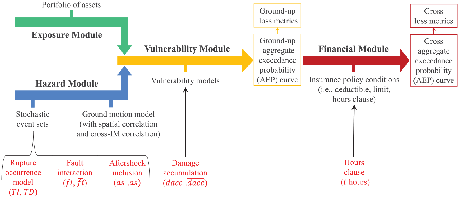
Flowchart of the event-based time-dependent earthquake risk assessment methodology used in this study. Time-dependent input options are displayed in red font.

The seismic hazard module generates stochastic event sets (i.e. synthetic catalogs of earthquake ruptures) based on simulated seismicity for the region of interest over a number of years. A number of time-dependent input modeling options that influence the stochastic event-set generation process are included and relate to: (1) fault rupture occurrence modeling (which can be either time-independent –TI– or time-dependent –TD); (2) fault-interaction modeling (included –fi– or not – $\overline{\mathrm{fi}}$ ); and (3) aftershock occurrence modeling (included –as– or not – $\overline{\mathrm{as}}$ ). The simulated earthquakes include rupture information required for the ground-motion intensity calculations (e.g. location, magnitude, and nodal planes). Consistent with the approach of Crowley and Silva (2013), one ground-motion field for each rupture is then simulated by sampling the probability distribution defined by a set of appropriate ground-motion models (GMMs), accounting for site effects. Spatial and cross-IM correlation models (e.g. Huang and Galasso, 2019; Jayaram and Baker, 2009; Weatherill et al., 2015) can be used to produce more accurate ground-motion fields.

The exposure module contains a portfolio of assets, which are mapped to specific building types. The taxonomy information is then used to select appropriate vulnerability models in the vulnerability module. These vulnerability models are used in conjunction with the ground-motion fields generated at each asset’s location to compute a set of ground-up (gu) loss metrics. The first of these metrics is LR_gu,a,e, which is the ground-up loss ratio (LR) for the ath asset and the eth earthquake obtained from the corresponding mean vulnerability model (where the loss ratio is the estimated repair cost divided by the asset’s replacement cost). Two alternative approaches to vulnerability modeling are considered for computing LR_gu,a,e:

• The approach used in conventional seismic risk assessments (indicated with $\overline{\mathrm{dacc}}$ ), in which the vulnerability calculations do not account for damage accumulation. This means that the vulnerability module has no memory of the building’s existing damage state (DS) due to previous events, and LR_gu,a,e is evaluated independently for each earthquake with the same vulnerability model (i.e. the assets are considered repaired immediately after each ground motion). In this approach, the annual ground-up losses of each asset can exceed their replacement cost (e.g. Iacoletti et al., 2023);

• The approach of Iacoletti et al. (2023) which makes use of the state-dependent vulnerability models to capture loss accumulation due to multiple ground motions (indicated with dacc). These vulnerability models define the LR_gu,a,e of an initially damaged building (i.e. which reached a certain $d{s}_j$ damage state during previous ground motions). In this approach, the annual ground-up losses of each asset cannot exceed their replacement cost (see Iacoletti et al., 2023, for more details).

The asset-level ground-up loss related to each earthquake, L_gu,a,e, is calculated by multiplying the LR_gu,a,e with the replacement cost of the ath asset. The portfolio ground-up loss for an earthquake, L_gu,e, is then the sum of all L_gu,a,e across the portfolio. The annual portfolio ground-up loss for each simulated year of the stochastic event set, L_gu, is calculated as the sum of the corresponding L_gu,e values. The ground-up aggregate exceedance probability (AEP) curve then provides the annual probability of L_gu exceeding a certain loss level and is determined as outlined in Crowley and Silva (2013). Ground-up AAL, AAL_gu, is calculated as the integral under the L_gu AEP curve. The L_gu corresponding to a prescribed RP X, in the L_gu AEP curve (denoted as the X-RP L_gu) is read directly from the curve.

The hours clause input option to the financial module is implemented for the ath asset, the nth simulated year of the stochastic event set, and t hours in the clause, according to the following procedure:

1. Identify the events simulated within the nth year;

2. Order the identified events according to their associated LR_gu,a,e value, from the highest to the lowest;

3. For each ordered event (referred to at this stage as a “payout event”), do the following:

This procedure is based on the idea that the event most likely “triggering” a claim is the one causing the largest loss to the policyholders (which might be different for each asset). However, this assumption might not be consistent with the practices of all insurers and reinsurers. The number of hours in a typical hours clause depends on the peril and is typically 168 for earthquakes (Mitchell-Wallace, 2017). Table 1 provides an example implementation of a 168-h clause. Event e2 is the first payout event since it is associated with the largest LR_gu,a,e. Events e3 and e4 are cumulative events of e2 because they occur within a 168-h time window. Event e5 is identified as the second payout event since it is associated with the second largest LR_gu,a,e value and did not feature as a cumulative event for e2. Events e6 and e7 are the corresponding cumulative events because they respectively occur within 44 and 140 h of event e5. The final payout events, e8 and e1, do not have any associated cumulative events. In a year like the one shown in Table 1, the insurer would have to pay a policyholder twice for the LR_gr,a,e caused by two clusters of events (regardless of whether the payout event in the cluster was a mainshock or an aftershock).

Table 1.

Example implementation of a 168-h clause for one asset in a simulated year.

Event ID	Decimal year	Hours from the start of the year	LRgu,a,e	LRgu,a,e for payout event e2	LRgu,a,e for payout event e5	Modified ${\mathrm{LR}}_{\mathrm{gu},a,e}^{*}$	LRgr,a,e
e1	1.007	61	0.020			0.020	0.000
e2	1.010	88	0.200	0.200 (p)		0.260	0.160
e3	1.025	219	0.040	0.040 (c)		0.000
e4	1.028	245	0.020	0.020 (c)		0.000
e5	1.560	4909	0.045		0.045 (p)	0.115	0.015
e6	1.565	4953	0.030		0.030 (c)	0.000
e7	1.576	5049	0.040		0.040 (c)	0.000
e8	1.580	5080	0.030			0.030	0.000

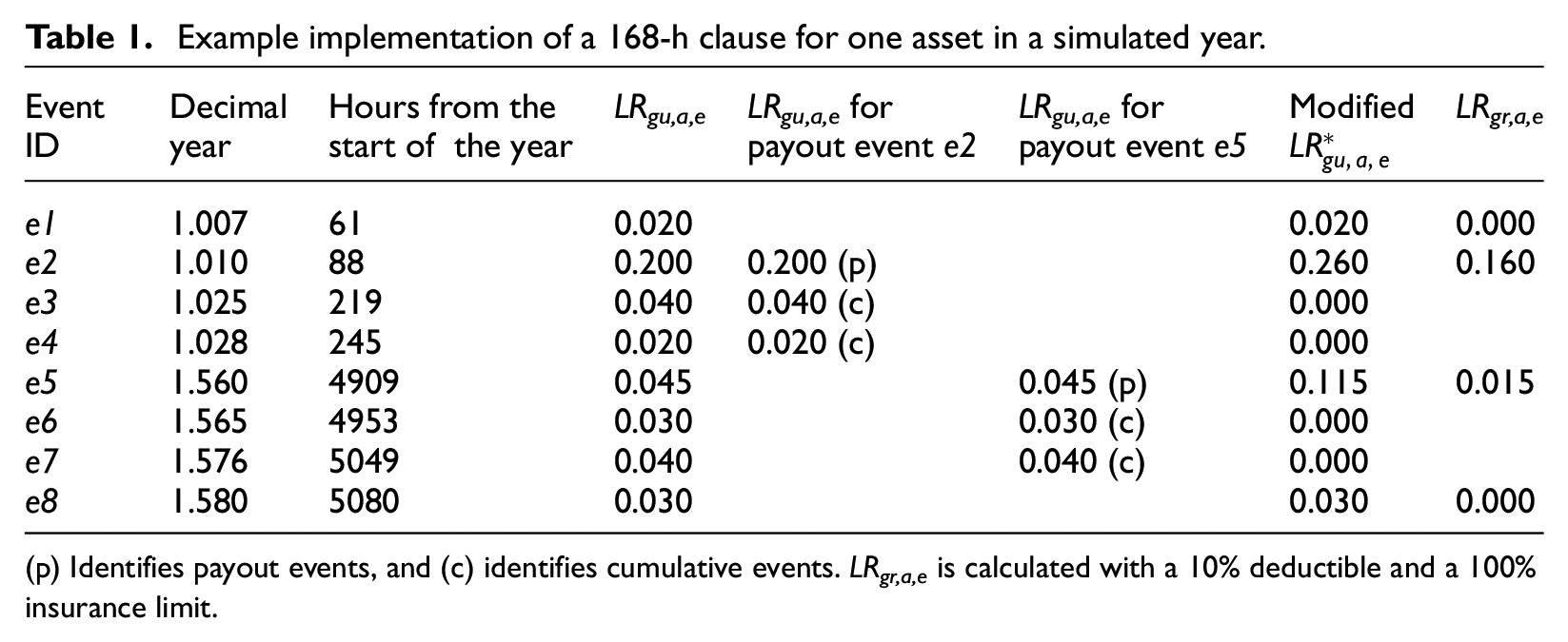
(p) Identifies payout events, and (c) identifies cumulative events. LR_gr,a,e is calculated with a 10% deductible and a 100% insurance limit.

Gross (gr) loss metrics are computed as the final output of the framework. The asset-level gross loss ratio, LR_gr,a,e, is calculated by applying insurance limits and deductibles to each asset’s ${\mathrm{LR}}_{\mathrm{gu},a,e}^{*}$ (i.e. the modified loss ratio). The deductible is the amount of loss a policyholder has to pay before reclaiming from the policy and is selected by insurance companies to avoid incurring running expenses with minor claims. Typical earthquake deductibles vary between 0% and 15% (Goda et al., 2015). The insurance limit is the maximum amount a policy will pay out. Most modern insurance contracts apply an insurance limit of 100% on customers. In this study, the deductible and the insurance limit are expressed as a percentage of the replacement cost. Extending the hours-clause window likely increases the number of cumulative events included within each window, therefore growing the chances of exceeding the deductible. This is consistent with the structure of real-life insurance policies. L_gr,a,e is calculated by multiplying the corresponding LR_gr,a,e with the replacement cost of the ath asset (where all variables are as previously defined). L_gr,e, L_gr, AAL_gr, and X-RP L_gr are calculated analogously to corresponding ground-up loss metrics. Insurance companies commonly also cede portions (or layers) of L_gr,e to reinsurance companies to limit the risk of incurring an exceedingly large loss for any given eth event.

Variance-based sensitivity analysis

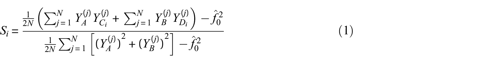
Variance-based sensitivity analysis is used to investigate the effects of introducing earthquake risk modeling time-dependent features on AAL_gu, AAL_gr, and X-RP L_gu outputs. For a given model of the form $Y=g(\mathbf{X})$ , variance-based methods quantify the sensitivity of Y to X in terms of a reduction in the variance of Y (e.g. Saltelli et al., 2010). In contrast to simpler sensitivity analysis methods (e.g. local sensitivity analyses depicted on tornado plots), variance-based sensitivity analyses provide quantitative sensitivity measures that consider the interaction among inputs X (Borgonovo and Plischke, 2016). In this study, Y is the loss metric of interest (such as AAL_gu or AAL_gr), the function $g(·)$ represents the methodology used in this study to calculate losses (described in the “Event-based time-dependent earthquake risk assessment framework” section), and X represents the time-dependent input options to be investigated. The first-order (main) sensitivity coefficient $S_i$ is used to estimate the contribution of the ith input to the output variance (i.e. it measures the effect of varying the ith input alone, averaged over variations in other inputs). $S_i$ values are calculated through the sampling procedure proposed by Saltelli et al. (2010). The logic-tree approach (e.g. Bommer and Scherbaum, 2008) is used to sample the considered time-dependent features, where each set of time-dependent input options (marked in red in Figure 1) corresponds to a section of the tree. In the absence of further information, all branches within a given section are equally weighted, which allows for general conclusions on the importance of different inputs to be drawn. Four matrices are developed from the samples produced: (1) A , built with N samples of each input of interest; (2) B containing another set of N samples generated in the same way as A ; (3) ${\mathit{C}}_i$ , built by substituting the ith column of matrix A for the ith column of matrix B ; and (4) ${\mathit{D}}_i$ , built by substituting the ith column of matrix B for the ith column of matrix A . The qth column of each matrix corresponds to a section of the logic tree. The pth row is a sampled set of branches from each section, used to generate K-years stochastic events sets and compute the loss metrics of interest. $Y_A$ , $Y_B$ , $Y_{C_i}$ , and $Y_{D_i}$ are the vectors of a given loss metric corresponding to A , B , ${\mathit{C}}_i$ , and ${\mathit{D}}_i$ , respectively. $S_i$ is then estimated as:

$$S_i=\frac{\frac{1}{2N}({\sum }_{j=1}^N{Y}_A^{(j)}{Y}_{C_i}^{(j)}+{\sum }_{j=1}^N{Y}_B^{(j)}{Y}_{D_i}^{(j)})-{\hat{f}}_0^2}{\frac{1}{2N}{\sum }_{j=1}^N[{(Y_A^{(j)})}^2+{(Y_B^{(j)})}^2]-{\hat{f}}_0^2}$$

(1)

where N is the number of generated samples, ${\hat{f}}_0^2=(1/2N){\sum }_{j=1}^N(Y_A^{(j)}{Y}_B^{(j)}+Y_{C_i}^{(j)}{Y}_{D_i}^{(j)})$ per Yun et al. (2017), and $Y_A^{(j)}$ , $Y_B^{(j)}$ , $Y_{C_i}^{(j)}$ , and $Y_{D_i}^{(j)}$ are the jth elements of $Y_A$ , $Y_B$ , $Y_{C_i}$ , and $Y_{D_i}$ , respectively. More details on variance-based sensitivity analysis can be found in Saltelli et al. (2010) and Cremen and Baker (2020).

Case study

The case study is contained within the bounding box of longitudes [13°, 13.9°] and latitudes [41.9°, 42.8°] in Central Italy (Figure 2). The sensitivity results are presented for the entire portfolio described in the “Exposure module” section, and for the cities of L’Aquila, Teramo, and Avezzano specifically (i.e. only considering assets in these cities), which collectively represent around 40% of the portfolio’s total replacement value.

Figure 2.

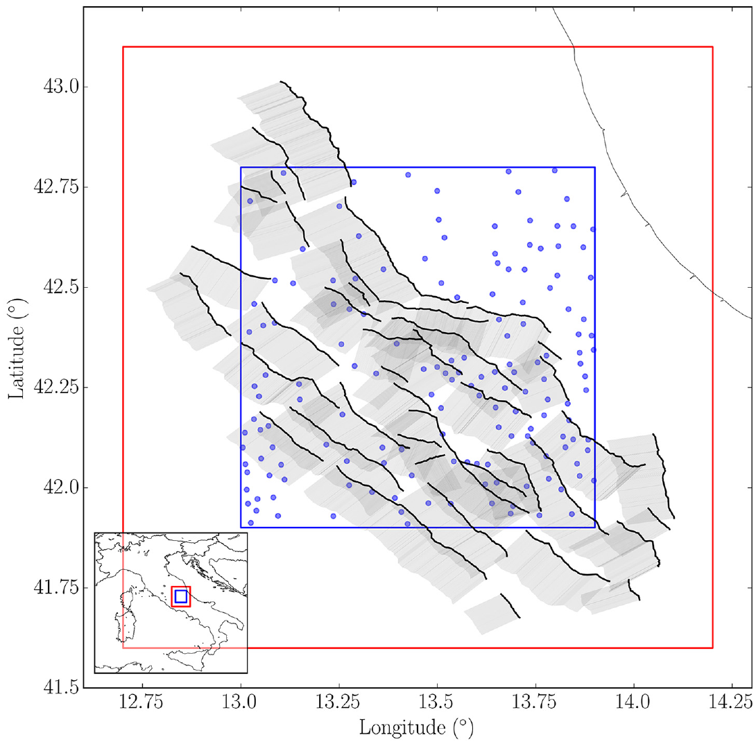
Case-study portfolio (subset of that presented in Crowley et al. (2021a), blue dots within the blue polygon, representing density-weighted centroids). The red polygon is the study area used in Iacoletti et al. (2022a) to generate the stochastic event sets. The 43 considered fault segments (Scotti et al., 2021) are shown in black (fault trace) and gray (geometry at depth).

Seismic hazard module

The stochastic event sets used in the case study have been developed by Iacoletti et al. (2022a) for Central Italy, within the bounding box of longitudes [12.6°, 14.2°] and latitudes [41.6°, 43.2°]. Iacoletti et al.’s (2022a) approach for stochastic event-set generation combines fault-based seismicity, distributed seismicity, and aftershocks simulated with a simulator based on the Epidemic-Type Aftershock Sequence (ETAS) model. Fault-based seismicity is simulated based on 43 fault segments (shown in Figure 2) from the Fault2SHA Central Appennines laboratory (Faure Walker et al., 2021; Scotti et al., 2021). Fault data required to calibrate the fault-based seismicity modeling component (i.e. slip rates, paleoseismic records, and date of the last event) are taken from the works by Scotti et al. (2021) and Valentini et al. (2019), and other available data sources (see Iacoletti et al., 2022a, for more details). One time-independent and three time-dependent fault rupture occurrence models are used. The time-dependent fault rupture occurrence models are based on the Brownian Passage Time (BPT; Matthews et al., 2002) model with different levels of recurrence uncertainty (Field et al., 2015): high $(\mathrm{TD}=\mathrm{BP}{\mathrm{T}}_{\mathrm{high}})$ , medium $(\mathrm{TD}=\mathrm{BP}{\mathrm{T}}_{\mathrm{mid}})$ , and low $(\mathrm{TD}=\mathrm{BP}{\mathrm{T}}_{\mathrm{low}})$ . The time-dependent fault rupture occurrence models account for the time elapsed since the last event when available; otherwise, the methodology proposed by Field and Jordan (2015) is applied. For more details, the reader is referred to Iacoletti et al. (2021). The fault system is considered to be unsegmented, following the methodology of UCERF3 (Field et al., 2014). Fault interaction is modeled by introducing a stress-based proxy (i.e. Coulomb stress changes; King et al., 1994) that modifies the rupture occurrence probabilities computed with the fault rupture occurrence model (Iacoletti et al., 2021; Toda et al., 1998). The “Catalogo Parametrico dei Terremoti Italiani” (CPTI15, Rovida et al., 2020) is used to calibrate the time-independent distributed seismicity model. The stochastic event-set generation also accounts for the initial stress state of the 43 considered fault segments, using information on stress built up by all $M_W\ge 6$ events in the CPTI15 and more recently until 2022, the starting year of the analysis (Iacoletti et al., 2022a). Aftershocks are generated with an ETAS-based simulator calibrated with the Homogenized Instrumental Seismic Catalog (HORUS, Lolli et al., 2020) according to Iacoletti et al. (2022b). The ETAS-based simulator is a modified version of the classic ETAS model (e.g. Ogata and Zhuang, 2006) that includes: (a) a truncated version of the Omori–Utsu law (Cattania et al., 2018; Utsu et al., 1995); (b) fault geometry information to account for the anisotropic spatial distribution of aftershocks (Guo et al., 2015); (c) a double-truncated magnitude-frequency distribution, as defined in Iacoletti et al. (2022a); and (d) short-term magnitude incompleteness (Page et al., 2016) to emulate the initial b-value decrease (e.g. Omi et al., 2014). Five years of historical seismicity before the simulation period (i.e. between 2017 and 2021) are used to account for the aftershocks due to past seismicity (Iacoletti et al., 2022a). The stochastic event sets that include aftershocks contain a slightly lower number of $5<M_W<5.5$ events than the undeclustered CPTI15 observed catalog (Iacoletti et al., 2022a). However, this is deemed a minor discrepancy and we consider them generally acceptable for the purpose of this study. The ground-motion fields are computed at each asset in the portfolio with the GMM developed by Cauzzi et al. (2015), and accounting for both spatial and cross-IM correlation using the procedure proposed by Markhvida et al. (2018). The site effects are accounted for using the mean $V_{S30}$ (shear-wave velocity in the upper 30 m) values from the map developed by Mori et al. (2020).

Exposure module

The case-study portfolio (shown in Figure 2) is a subset of the ESRM20 residential building portfolio for Italy, which was developed using 2011 public census data provided by the Department of Civil Protection (Crowley et al., 2020, 2021a). The number of buildings and associated total replacement costs (structural, non-structural, and contents) of this portfolio are aggregated at Administrative Level 3 (i.e. roughly equivalent to a township or a municipality) and represented by a density-weighted centroid, which is calculated from the built-up area density map (Crowley et al., 2021a; Dabbeek et al., 2021). Each centroid is associated with assets of different building types (classes), which describe the material and type of the lateral load-resisting system, the seismic code or ductility level, and the building height (in terms of number of stories). This case-study portfolio contains around 136,000 buildings, representing 8188 asset entries, 157 unique locations, 32 different building types, and a total replacement cost of €27.4 billion. A summary of the ESRM20 residential building classes that feature in the case-study portfolio is provided in Table 2.

Table 2.

Building classes in the case-study exposure model (see “Data and resources” section for more information).

Building class	Description
CR-LFINF-CDL-FY-HX	Reinforced concrete (CR) building with infilled frames (LFINF), low-code level (CDL, designed for lateral resistance using allowable stress design), FY = 0%, 5%, or 10%, HX = 1–4 stories (H1–H4)
CR-LFINF-CDM-FY-HX	Reinforced concrete (CR) building with infilled frames (LFINF), moderate-code level (CDM, designed for lateral resistance with modern limit state design), FY = 0%, 5%, or 10%, HX = 1–4 stories (H1–H4)
MCF-LWAL-DUL-HX	Confined masonry (MCF) building with load-bearing walls (LWAL), low ductility (DUL), HX = 1–4 stories (H1–H4)
MUR-STRUB-LWAL-DNO-HX	Rubble stone masonry (MUR-STRUB) building with load-bearing walls (LWAL), non-ductile (DNO), HX = 1–3 stories (H1–H3)
MUR-STDRE-LWAL-DNO-H4	Dressed stone masonry (MUR-STDRE) building with load-bearing walls (LWAL), non-ductile (DNO), 4 stories (H4)

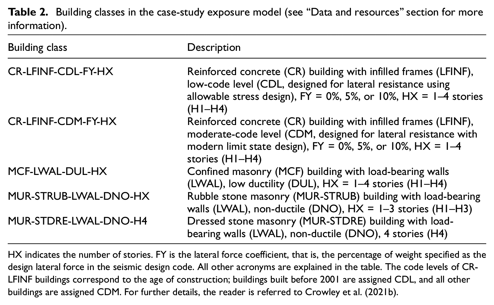
HX indicates the number of stories. FY is the lateral force coefficient, that is, the percentage of weight specified as the design lateral force in the seismic design code. All other acronyms are explained in the table. The code levels of CR-LFINF buildings correspond to the age of construction; buildings built before 2001 are assigned CDL, and all other buildings are assigned CDM. For further details, the reader is referred to Crowley et al. (2021b).

Vulnerability module

We use the suite of single-ground-motion (i.e. mainshock-only) and state-dependent vulnerability models developed by Iacoletti et al. (2023) for the building types used in this study (available at https://github.com/SalvIac/sequence_frag_vuln). These models have been developed based on the energy-based probabilistic seismic demand model by Gentile and Galasso (2021), which is a physically consistent model that accounts for the accumulation of damage (even though it is solely based on numerical analyses and requires further experimental/field validation). The IM associated with each state-dependent and single-ground-motion vulnerability model is the average spectral acceleration at a range of periods of interest (which vary for each building type), calculated from the capacity curve associated with each taxonomy (Iacoletti et al., 2023; Martins and Silva, 2021). Each state-dependent vulnerability model is conditional on the previous $d{s}_j$ reached, ranging from $d{s}_0$ to $d{s}_3$ , representing no $(d{s}_0)$ , slight $(d{s}_1)$ , moderate $(d{s}_2)$ , or extensive $(d{s}_3)$ damage (Iacoletti et al., 2023). The approach proposed in Iacoletti et al. (2023) is used in this study to capture loss accumulation due to multiple ground motions (i.e. dacc branches).

Ground-up losses

Figure 3 provides the uniformly weighted logic tree of time-dependent input options investigated. The number of samples N and the number of years K of generated seismicity are case-study-dependent and affect the computational time needed to run the sensitivity analysis. For this study, $N=2000$ and $K=10000$ yr have been selected after several tests, which provide a reasonable compromise between the numerical stability of the $S_i$ values and the computational cost required. Figure 4 displays the L_gu AEP curves for a set of logic-tree branches (i.e. $\overline{\mathrm{as}}-\overline{\mathrm{dacc}}-\mathrm{TI}-\overline{\mathrm{fi}}$ , $\overline{\mathrm{as}}-\overline{\mathrm{dacc}}-\mathrm{BP}{\mathrm{T}}_{\mathrm{mid}}-\overline{\mathrm{fi}}$ , and $\mathrm{as}-\mathrm{dacc}-\mathrm{BP}{\mathrm{T}}_{\mathrm{mid}}-\mathrm{fi}$ ), and the range of variability of these curves across all logic-tree branches. Figure 4 also provides the ratio (for each specific annual probability of exceedance) of the $\mathrm{as}-\mathrm{dacc}-\mathrm{BP}{\mathrm{T}}_{\mathrm{mid}}-\mathrm{fi}$ and $\overline{\mathrm{as}}-\overline{\mathrm{dacc}}-\mathrm{BP}{\mathrm{T}}_{\mathrm{mid}}-\overline{\mathrm{fi}}$ curves with respect to that of $\overline{\mathrm{as}}-\overline{\mathrm{dacc}}-\mathrm{TI}-\overline{\mathrm{fi}}$ . The time-dependent fault rupture occurrence model leads to lower values of L_gu in general; the AAL_gu for $\overline{\mathrm{as}}-\overline{\mathrm{dacc}}-\mathrm{BP}{\mathrm{T}}_{\mathrm{mid}}-\overline{\mathrm{fi}}$ is approximately 9% less than that for $\overline{\mathrm{as}}-\overline{\mathrm{dacc}}-\mathrm{TI}-\overline{\mathrm{fi}}$ . This is because the time-dependent rupture occurrence probability of the considered fault system in Central Italy is lower than that calculated with a time-independent model (Iacoletti et al., 2022a). Aftershock inclusion, fault interaction, and the inclusion of state-dependent vulnerability calculations (denoted by $\mathrm{as}-\mathrm{dacc}-\mathrm{BP}{\mathrm{T}}_{\mathrm{mid}}-\mathrm{fi}$ ) lead to an increase in AAL_gu of around 22% and an increase of approximately 25% in the 200-year-RP L_gu, relative to the respective values obtained for $\overline{\mathrm{as}}-\overline{\mathrm{dacc}}-\mathrm{BP}{\mathrm{T}}_{\mathrm{mid}}-\overline{\mathrm{fi}}$ . These increases are predominantly due to the inclusion of aftershocks, which considerably amplify hazard (and potential losses) following relatively large-magnitude mainshocks.

Figure 3.

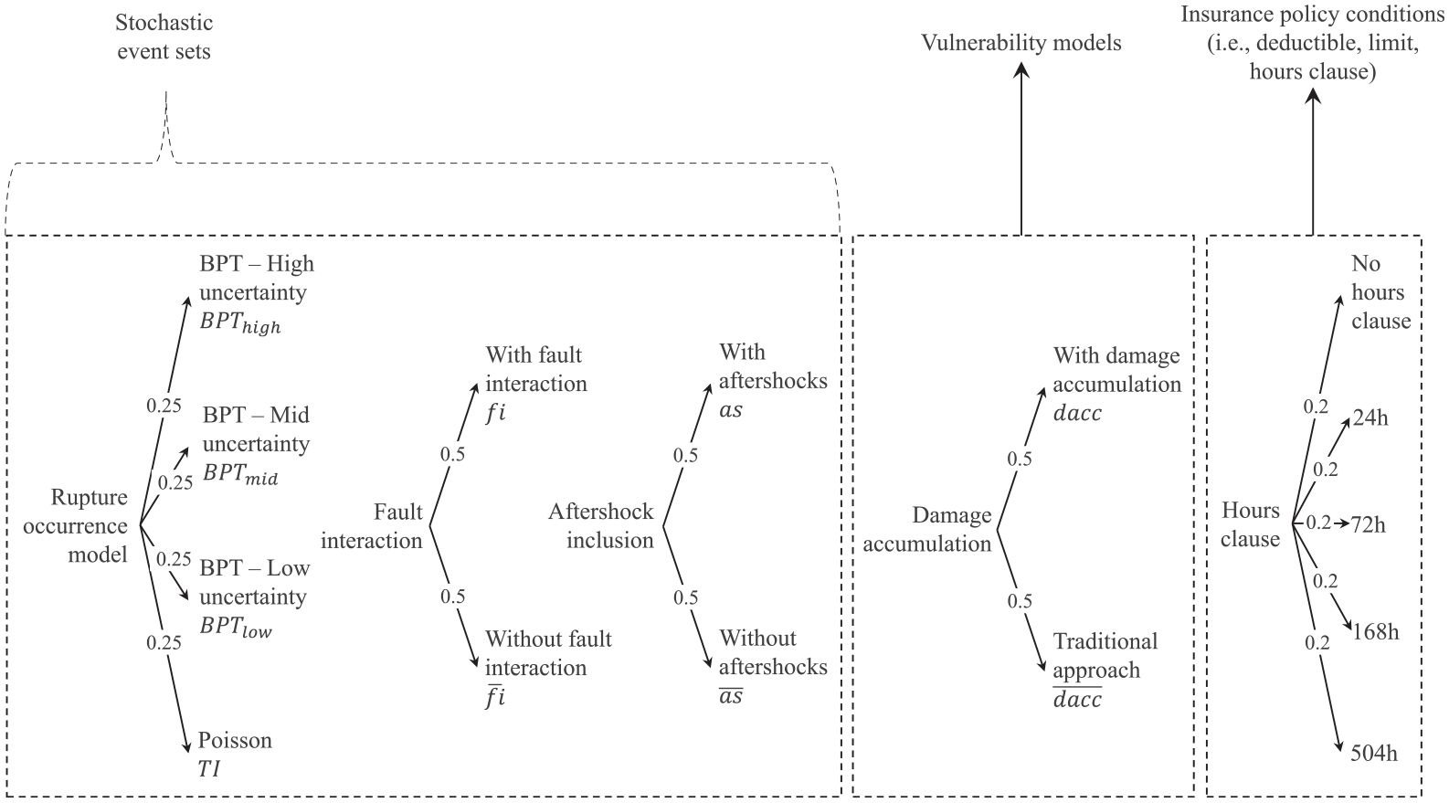
Logic tree used in the sensitivity analysis.

Figure 4.

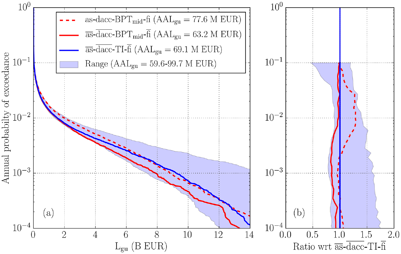
(a) L_gu AEP curves for $\overline{\mathrm{as}}-\overline{\mathrm{dacc}}-\mathrm{TI}-\overline{\mathrm{fi}}$ , $\overline{\mathrm{as}}-\overline{\mathrm{dacc}}-\mathrm{BP}{\mathrm{T}}_{\mathrm{mid}}-\overline{\mathrm{fi}}$ , and ${\mathrm{as}-\mathrm{dacc}-\mathrm{BPT}}_{\mathrm{mid}}-$ fi, and the range of variability across logic-tree branches. (b) Ratio (for each specific annual probability of exceedance) of the ${\mathrm{as}-\mathrm{dacc}-\mathrm{BPT}}_{\mathrm{mid}}-$ fi and $\overline{\mathrm{as}}-\overline{\mathrm{dacc}}-\mathrm{BP}{\mathrm{T}}_{\mathrm{mid}}-\overline{\mathrm{fi}}$ AEP curves with respect to the corresponding curve for $\overline{\mathrm{as}}-\overline{\mathrm{dacc}}-\mathrm{TI}-\overline{\mathrm{fi}}$ , and the range of variability of these ratios across the considered logic-tree branches. TI and $\mathrm{BP}{\mathrm{T}}_{\mathrm{mid}}$ are time-independent and time-dependent (with mid recurrence uncertainty) fault rupture occurrence models, respectively; fi and $\overline{\mathrm{fi}}$ respectively indicate the consideration of fault interaction and not; as and $\overline{\mathrm{as}}$ respectively indicate the inclusion and non-inclusion of aftershocks; dacc and $\overline{\mathrm{dacc}}$ respectively indicate the consideration of damage accumulation or not.

Figure 5 provides $S_i$ values associated with AAL_gu and 2500-year RP L_gu (denoted as $S_{i,\mathrm{AA}{L}_{\mathrm{gu}}}$ and $S_{i,\mathrm{RP}{2500}_{\mathrm{gu}}}$ , respectively) for the cities of L’Aquila, Teramo, and Avezzano, and the entire portfolio. $S_i$ values associated with fault-interaction modeling are close to negligible in all cases. This is consistent with the findings of Iacoletti et al. (2022a) for the same region. It is explained by the fact that typical ruptures generated by the 43 considered fault segments (Figure 2) cannot produce stress changes large enough to affect the occurrence probabilities of other ruptures (Iacoletti et al., 2021). However, this result is highly dependent on the specific details of the case study, including fault geometry and earthquake magnitudes (e.g. Iacoletti et al., 2022c). The $S_{i,\mathrm{AA}{L}_{\mathrm{gu}}}$ values associated with vulnerability modeling are generally small. The corresponding $S_{i,\mathrm{RP}{2500}_{\mathrm{gu}}}$ values are larger, implying that the consideration (or not) of damage accumulation is more important in the tail of the L_gu AEP curve (corresponding to high RP L_gu values). The AAL_gu and 2500-year RP L_gu are most sensitive to variations in the fault rupture occurrence models (i.e. time-dependent versus time-independent model) and the inclusion (or not) of aftershocks.

Figure 5.

$S_{i,\mathrm{AA}{L}_{\mathrm{gu}}}$ and $S_{i,\mathrm{RP}{2500}_{\mathrm{gu}}}$ values for the cities of L’Aquila, Teramo, and Avezzano and the full case-study portfolio.

At L’Aquila, the highest $S_{i,\mathrm{AA}{L}_{\mathrm{gu}}}$ and $S_{i,\mathrm{RP}{2500}_{\mathrm{gu}}}$ values are associated with fault rupture occurrence modeling. This is because time-dependent seismic hazard is expected to be notably lower than time-independent hazard at this location, due to the rupture of the Paganica fault in 2009 (e.g. Iacoletti et al., 2022a; Pace et al., 2016). At Teramo, the highest $S_{i,\mathrm{AA}{L}_{\mathrm{gu}}}$ values are associated with aftershock modeling and fault rupture occurrence modeling and the highest $S_{i,\mathrm{RP}{2500}_{\mathrm{gu}}}$ is associated with fault rupture occurrence modeling. For Avezzano and for the overall portfolio, the highest $S_{i,\mathrm{AA}{L}_{\mathrm{gu}}}$ and $S_{i,\mathrm{RP}{2500}_{\mathrm{gu}}}$ values are associated with aftershock modeling (although the overall portfolio $S_{i,\mathrm{RP}{2500}_{\mathrm{gu}}}$ value for fault rupture occurrence modeling is similar to that for aftershock modeling). The 2500-year RP L_gu of the overall portfolio is more sensitive than the AAL_gu to variations in the fault rupture occurrence modeling. This reflects the fact that the choice of fault rupture occurrence model affects rare, longer-term hazard estimates the most (Iacoletti et al., 2022a). The inclusion or not of aftershocks affects short-term hazard estimates, which helps to explain why the $S_{i,\mathrm{AA}{L}_{\mathrm{gu}}}$ value associated with aftershock modeling is generally higher than the corresponding $S_{i,\mathrm{RP}{2500}_{\mathrm{gu}}}$ value.

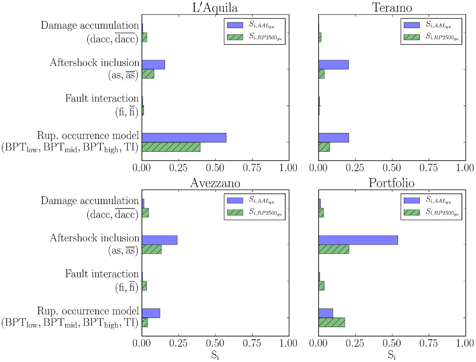
The sensitivity analysis for AAL_gu is repeated at each centroid of the portfolio (see Figure 2) separately to explore the spatial variability of corresponding $S_{i,\mathrm{AA}{L}_{\mathrm{gu}}}$ values. Figure 6a displays a map of the time-dependent input options associated with the highest $S_{i,\mathrm{AA}{L}_{\mathrm{gu}}}$ for each centroid. The consideration or not of aftershocks represents the highest contribution to the variance of the AAL_gu (i.e. the loss metric is most sensitive to the “aftershock inclusion” logic-tree branching level in Figure 3) in most of the study area (around 73%), and the loss metric is most sensitive to the choice of long-term fault rupture occurrence model across the remaining area. The sensitivity of AAL_gu to variations in the fault rupture occurrence model is highest where the considered site is close to a fault segment that recently ruptured (see Figure 6b) or located in an area with high background seismicity (northwest portion of the study area, see Figure 5 of Iacoletti et al., 2022a); this is also clear from Figure 6c, which plots the ratio of the $S_{i,\mathrm{AA}{L}_{\mathrm{gu}}}$ value associated with aftershock modeling and that associated with fault rupture occurrence modeling, for each centroid. This is because close to a fault segment that recently ruptured, the time-dependent fault rupture occurrence models produce significantly lower occurrence probabilities than the time-independent model (e.g. Polidoro et al., 2012). In areas where the background seismicity is high, large-magnitude mainshocks occur relatively often (compared to areas with low background seismicity) and dominate over aftershocks in terms of seismic hazard.

Figure 6.

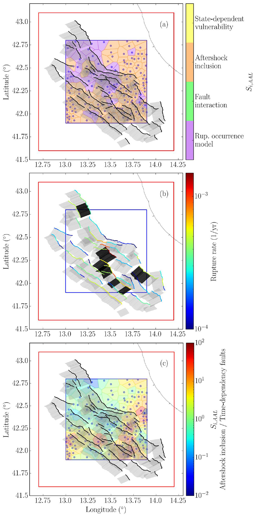
Maps of (a) the time-dependent input option associated with the highest $S_{i,\mathrm{AA}{L}_{\mathrm{gu}}}$ for each centroid and (b) the fault system in the study area and rupture rates. Fault segments that recently ruptured are shown in black. (c) Ratios between the $S_{i,\mathrm{AA}{L}_{\mathrm{gu}}}$ associated with aftershock modeling and those associated with fault rupture occurrence modeling, across each centroid.

Gross losses

The sensitivity of gross losses is investigated for 5-h-clause windows (see Figure 3): 0 (equivalent to no hours clause), 24, 72, 168, and 504 h, using three levels of deductible (set respectively as 0.1%, 1%, and 10% of the replacement cost of each asset). The insurance limit is set to 100% of the replacement cost of each asset. Reinsurance considerations are neglected in this study for simplicity.

Figure 7 demonstrates the effect of different hours-clause windows and deductibles on AAL_gr, for sets of logic-tree branches that include aftershocks (as). The AAL_gr increases (with a decreasing gradient) as the hours-clause window increases and more (cumulative) event losses are accounted for. The decreasing gradient reflects the decreasing rate of aftershocks over time (Utsu et al., 1995).

Figure 7.

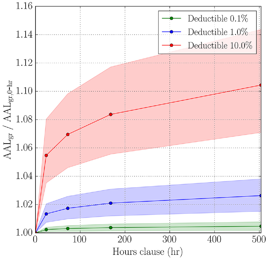
Ratio between AAL_gr and $\mathrm{AA}{L}_{\mathrm{gr},0-\mathrm{hr}}$ (i.e. corresponding to a 0-h clause) across different hours-clause windows and deductible levels, for sets of logic-tree branches that include aftershocks (as). Curves are linearly interpolated between 0, 24, 72, 168, and 504 h. The solid lines and shaded areas respectively represent the mean and range of $\mathrm{AA}{L}_{\mathrm{gr}}/\mathrm{AA}{L}_{\mathrm{gr},0-\mathrm{hr}}$ across the considered sets of logic-tree branches, for a specific deductible level.

Figure 8 displays the effect of different hours-clause windows on the L_gr AEP curve, for the most complex set of logic-tree branches (i.e. $\mathrm{as}-\mathrm{dacc}-\mathrm{BP}{\mathrm{T}}_{\mathrm{mid}}-\mathrm{fi}$ ), using a 10% deductible. It can be seen that the variation in AAL_gr with the length of the hours-clause window is significantly lower than the range of AAL_gr variability across all possible sets of logic-tree branches presented in Figure 3.

Figure 8.

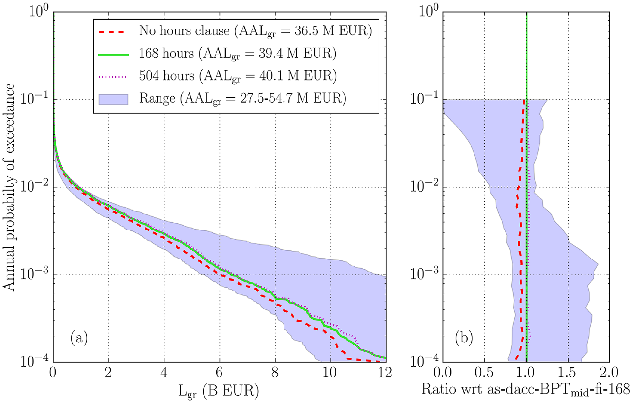
(a) L_gr AEP curves for $\mathrm{as}-\mathrm{dacc}-\mathrm{BP}{\mathrm{T}}_{\mathrm{mid}}-\mathrm{fi}$ , using different hours-clause windows and a 10% deductible. Also shown is the range of variability of the L_gr AEP curves across all possible sets of logic-tree branches in Figure 3. (b) Ratio (for each specific annual probability of exceedance) of the L_gr AEP curves in (a) with respect to the L_gr AEP curve for $\mathrm{as}-\mathrm{dacc}-\mathrm{BP}{\mathrm{T}}_{\mathrm{mid}}-\mathrm{fi}-168$ (with 168-h clause), and the range of variability of these ratios across all possible sets of logic-tree branches considered.

Figure 9 provides the $S_i$ values associated with AAL_gr for the entire portfolio, across different deductible levels investigated and all possible sets of logic-tree branches (denoted in blue). Consistent with the findings for the ground-up loss metrics, the consideration of fault interaction has a limited effect on the variance of AAL_gr. The $S_{i,\mathrm{AA}{L}_{\mathrm{gr}}}$ values associated with fault rupture occurrence modeling remain reasonably constant across different deductible levels and indicate that AAL_gr is as sensitive as AAL_gu to this modeling feature. The $S_{i,\mathrm{AA}{L}_{\mathrm{gr}}}$ value associated with the hours clause is generally low and increases with deductible level (in accordance with Figure 7). The $S_{i,\mathrm{AA}{L}_{\mathrm{gr}}}$ values associated with aftershock modeling are relatively high, except for a 10% deductible level. This is because higher deductibles are less frequently exceeded for aftershocks (than for mainshocks). The $S_{i,\mathrm{AA}{L}_{\mathrm{gr}}}$ associated with vulnerability modeling is highest (and notable) for a 10% deductible because this deductible level is more frequently exceeded when damage accumulation is accounted for.

Figure 9.

$S_{i,\mathrm{AA}{L}_{\mathrm{gr}}}$ for the entire case-study portfolio and different deductibles.

The sensitivity analysis is repeated to further explore $S_{i,\mathrm{AA}{L}_{\mathrm{gr}}}$ in the presence of aftershock modeling (i.e. only considering sets of logic-tree branches that include as), given the dominant variance contribution of the $\{\mathrm{as},\overline{\mathrm{as}}\}$ logic-tree section to AAL_gr. Fixing the as branch will produce larger $S_{i,\mathrm{AA}{L}_{\mathrm{gr}}}$ values for the other sections of the logic tree (due to the removal of first- and higher-order interaction effects associated with uncertainty in aftershock inclusion) but the extent of the increase for each value may not be equivalent. The updated $S_{i,\mathrm{AA}{L}_{\mathrm{gr}}}$ values are found to rank similarly to those obtained for all possible sets of logic-tree branches (see green bars in Figure 9). The only minor difference is that the lowest $S_{i,\mathrm{AA}{L}_{\mathrm{gr}}}$ value is associated with fault interaction (instead of the hours clause) for a 10% deductible level, which does not change the overall conclusions.

Conclusions

This study explored the sensitivity of a selection of monetary loss metrics to various time dependencies often neglected in conventional earthquake risk models. An event-based time-dependent earthquake risk assessment methodology was used for the sensitivity analysis, accounting for long-term time-dependent rupture occurrences that include the effects of fault interaction, short-term hazard increases caused by aftershocks, and damage accumulation in assets due to multiple ground motions occurring in a short time period. The investigation was designed to provide important insights for the catastrophe insurance and reinsurance industry, so specific insurance features (e.g. hours clauses) were also considered in the calculations. A sample portfolio in Central Italy, including the cities of L’Aquila, Teramo, and Avezzano, was used as a case study for the investigation.

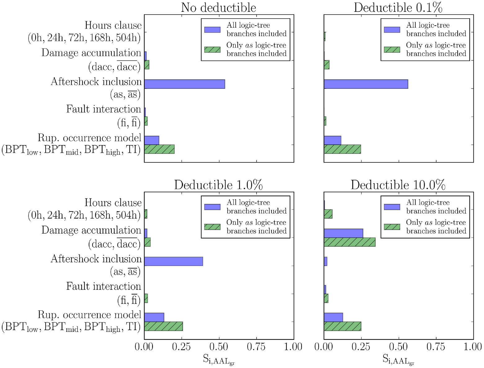
The sensitivity analysis revealed that the AAL_gu and 2500-year-RP L_gu loss metrics are most sensitive to the choice of long-term fault rupture occurrence model and whether or not aftershocks are accounted for. Thus, these two modeling features are the most important to constrain when developing a time-dependent seismic risk model (at least for the case study investigated). AAL_gu is generally more sensitive to the modeling of aftershocks than 2500-year-RP L_gu. This is because aftershocks increase the short-term hazard estimates and corresponding losses at low RP. Time-dependent fault rupture occurrence models can also significantly affect AAL_gu close to a fault that recently ruptured (e.g. at L’Aquila). The sensitivity of specific-RP L_gu to aftershock modeling and fault rupture occurrence modeling respectively decreases and increases with increasing RP. This means that the choice of fault rupture occurrence model is more important than the consideration of aftershocks for large-RP L_gu (including the 2500-year-RP L_gu metric specifically examined). The sensitivity of the loss metrics to the modeling of vulnerability is relatively low but increases with increasing RP and larger losses produced by subsequent aftershocks. However, the fragility/vulnerability models used in this study are based on a probabilistic seismic demand model that has not been validated using experimental or field data, which could have affected the sensitivity results. Therefore, the effects of damage accumulation on risk obtained in this study should be treated as illustrative only. The sensitivity of the ground-up loss metrics to fault interaction is low, such that this modeling feature is the least important to constrain in a time-dependent seismic risk model.

The sensitivity results are generally similar in the case of gross losses; the long-term rupture occurrence and aftershock modeling components are also the most crucial to constrain for AAL_gr. However, if there is a high deductible level associated with portfolio assets (around 10%, as considered for the case study), then accounting for damage accumulation also becomes important. The sensitivity of AAL_gr to the length of the hours clause is generally relatively low.

The findings of this study focus on the sensitivity of relative loss metrics rather than absolute loss estimates and are limited in applicability to the case study, the logic-tree structure, and the underlying methodologies and assumptions. For instance, the calculation of L_gr depends on the implementation details of the hours clause. The process insurers use for assigning loss claims to specific hours or events is not standardized across the industry; the implementation procedure could be refined to better match the practices of specific insurers. The methodology used in this study could be extended by additionally considering reinsurance (and associated reinstatement clauses). Adopting alternative hazard modeling or damage accumulation methods, and/or focusing on another case-study region (where, for instance, fault interaction has higher impacts, e.g. California, King et al., 1994), could lead to different sensitivity results. Nevertheless, the sensitivity results obtained provide some valuable guidance on the treatment and importance of time dependencies in advanced large-scale (i.e. portfolio) earthquake risk models.