Sage Journals: Discover world-class research

Abstract

This article proposes a framework to support postearthquake building safety and reoccupancy decisions by quantifying the change in building collapse risk following a mainshock earthquake event. This risk may be exacerbated by both an increase in seismic hazard due to aftershock activity and a reduction in building collapse resistance due to structural damage. To address these factors, the framework is based on a hazard that includes (1) both the steady-state and the aftershock occurrence rates, that is, the elevated hazard that accounts for the dependence on the mainshock magnitude and the aftershock rate that decays over time, and (2) revised collapse fragility functions that account for structural damage sustained during the mainshock. The framework is capable of addressing region-specific questions such as (1) What are the mainshock magnitudes for which aftershocks pose a life-safety concern? (2) How long does it take for the elevated risk due to aftershocks to dissipate? and (3) What gaps in current knowledge deserve further attention from the earthquake engineering and seismology communities? The framework addresses these questions for a 20-story building in San Francisco, assuming three different, hypothetical mainshock events of magnitudes 7,7.5, and 8M_W on the San Andreas fault. This is followed by a parametric study that considers a range of buildings and provides a graphical representation of the elevated risk to inform building evaluation (tagging) decisions, based on the intact building’s collapse capacity, the amount of structural damage, and the length of time after the mainshock.

Keywords

Aftershock damaged building risk of collapse postearthquake safety decisions

Introduction

One of the first steps toward recovery following an earthquake is determining whether the buildings are safe to reoccupy. This decision typically focuses on the observed building damage, without explicitly considering increased seismic hazard due to aftershock activity. The internationally recognized building evaluation guidance, ATC-20-1 (2015), offers a qualitative assessment of whether the damage has significantly reduced a building’s collapse capacity, relative to its intact condition. When damage is significant, buildings are “red-tagged,” prohibiting reoccupancy until a more detailed evaluation is made and/or the damage is repaired. Moreover, heavily damaged buildings may trigger a safety cordon (a temporary barricade), restricting access to neighboring streets and buildings. With a few exceptions, described later, much of the existing research on quantitative measures to guide building evaluations focuses on relating the degree of damage to reductions in collapse capacity (e.g. Burton and Deierlein, 2018; Luco et al., 2004; Raghunandan et al., 2015).

Some studies have explicitly linked tagging decisions to the risk of collapse by including the time-dependent ground motion hazard, in addition to the building collapse capacity. Bazzurro et al. (2004) demonstrated this concept for on the steady-state hazard and referred to the work by Yeo and Cornell (2004) for modifying the tagging decision to incorporate the additional aftershock hazard that decays over time. The difference between the steady-state and aftershock hazards arises from the conventional representation of seismic hazard as constant in time. This steady-state model assumes a Poisson process for the rate of occurrence, where the time interval between each event is random and independent, yet the average interval is known. The aftershocks that follow a mainshock disrupt this Poissonian assumption. To characterize the Poisson model for mainshocks, “clusters” of aftershocks that are spatially and temporally linked to mainshocks are removed from the event catalog (e.g. Gardner and Knopoff, 1974). These aftershocks produce additional shaking that is not included in the steady-state hazard curve, but which can be accounted for through other models.

Yeo and Cornell (2009) developed a methodology for aftershock probabilistic site hazard analysis (APSHA). The formulation mirrors the traditional PSHA for the steady-state hazard by substituting the Poissonian rate of mainshock events with a time-dependent rate of aftershock events. This rate is based on several models that collectively consider the decaying rate of aftershocks, conditioned on the mainshock event (Gutenberg and Richter, 1944; Omori, 1894; Reasenberg and Jones, 1989; Utsu, 1961). Recent aftershock collapse risk assessment studies have used the Yeo and Cornell (2009) APSHA model to determine a hazard curve that reflects the aftershock environment (Iervolino et al., 2020; Shi et al., 2020; Shokrabadi and Burton, 2018; Zhang et al., 2019). The Yeo and Cornell (2009) APSHA framework only captures the aftershock portion of the hazard; therefore, one needs to add the steady-state component to provide a complete picture of the seismic hazard after a mainshock. Other aftershock hazard frameworks exist in the literature and consider the combined hazard due to both mainshock and aftershock events (Boyd, 2012; Iervolino et al., 2020; Toro and Silva, 2001). With such approaches, the hazard results include all of the possible shaking intensities from aftershock clusters associated with each Poissonian mainshock. For the purpose of informing safety decisions following a specified mainshock scenario, the Yeo and Cornell (2009) framework is more useful because it enables one to focus the hazard analysis on the earthquake cluster following the mainshock of interest.

There are a limited number of studies that consider an aftershock environment’s increased shaking hazard coupled with the reduction in collapse capacity due to structural damage sustained during a mainshock. Jalayer and Ebrahimian (2017) estimates the limit state exceedance probability for a structure subjected to successive shaking events. This method quantifies the fragility of the structure in terms of a continuous performance variable that is not directly associated with collapse. In contrast, Galvis et al. (2023) offered a simulation approach that uses sequential nonlinear response history analyses (NLRHA) to explicitly quantify the destabilizing effects of simulated damage on the collapse capacity. Similar methods have also been proposed by other authors (Burton and Deierlein, 2018; Goda and Taylor, 2012; Zhang et al., 2019). This detailed simulation approach allows for adjustments to the intact collapse fragility function as a function of damage indicators (DIs) that are observable after the mainshock.

The elevated collapse risk framework proposed in this study uses the elevated hazard (combination of the aftershock and steady-state hazards) with collapse fragility functions that account for mainshock damage. Together, these models provide a more complete collapse risk assessment in an aftershock environment. The framework is depicted in Figure 1 as three main modules, quantifying the elevated hazard conditioned on a mainshock event (M1), the collapse performance of a damaged building (M2), and the resulting elevated collapse risk (M3). The following sections present these modules through illustrative case studies for three hypothetical mainshock events near San Francisco, considering an individual 20-story building and a parametric study for an inventory of buildings. These case studies are instrumental for (1) identifying the mainshock magnitudes that pose a relevant aftershock concern and (2) probabilistically quantifying how long the collapse risk is elevated over the steady-state risk, allowing stakeholders to have informed discussions about disaster response activities. The case studies also highlight important gaps in current knowledge that deserve further attention and research. This article is accompanied by a supplemental document to examine the sensitivity of the case study results to a number of model and parameter choices that are used in the study.

Figure 1.

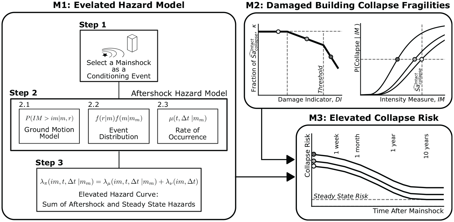
The proposed framework’s three modules, quantifying the elevated hazard (M1), the building collapse performance (M2), and the elevated collapse risk (M3).

Elevated hazard model (module 1)

The elevated hazard model is an extension of the Yeo and Cornell (2009) APSHA model. Whereas Yeo and Cornell’s APSHA model focuses primarily on the aftershock hazard, the proposed model also includes steady-state mainshock events, following the three steps diagrammed in module 1 of Figure 1. The following sections describe each of these steps, using an example site in downtown San Francisco to illustrate the procedure.

Step 1: select a mainshock as a conditioning event

The APSHA is based on an individual mainshock as a conditioning event. While Yeo and Cornell (2009) used idealized fault geometry for mainshocks of increasing magnitude, this study uses known fault geometries when selecting the conditioning mainshocks. San Francisco’s seismic hazard is primarily driven by the Hayward and San Andreas Faults (Aagaard et al., 2016). 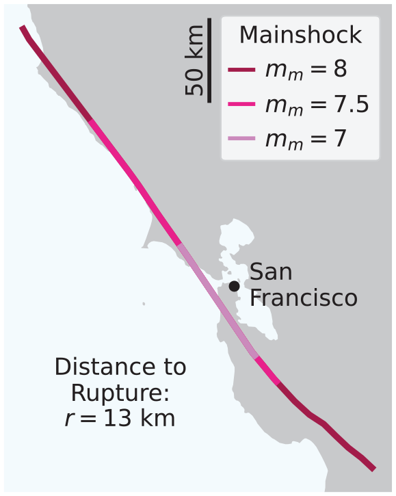The case study focuses on an earthquake on the San Andreas Fault, which was selected due to its proximity to downtown San Francisco and the fact that it could generate rupture magnitudes of up to $8 M_{W}$ . Figure 2 maps the case study’s mainshock rupture magnitudes of $m_{m} = 7, 7.5, and 8$ , with each rupture straddling the portion of the fault closest to downtown San Francisco. Selecting mainshock and aftershock ruptures at this location represent rather conservative scenarios. The exact rupture locations were selected from OpenSHA’s discrete event set for uniform California earthquake rupture forecast, Version 2 (UCERF2) (Field et al., 2008).

Figure 2.

The aftershock hazard analysis is conditioned a mainshock event, shown here for three different ruptures with magnitudes $m_{m} = 7, 7.5, and 8$ . Each mainshock rupture occurs on the San Andreas Fault, straddling the portion of the fault $r = 13 km$ away from downtown San Francisco.

The mainshock event conditions the aftershock environment in two ways: (1) the rate of aftershocks and (2) the event distribution with respect to aftershock magnitude and location (Utsu, 1969, 1971). The general concept of unique aftershock environments for each mainshock is discussed in the context of the Reasenberg and Jones (1989) model. This model combines the modified Omori’s law, $n (t) = K (t + c)^{- p}$ (Utsu, 1961), with the Gutenberg–Richter recurrence law, $λ_{m} = 10^{(a - bm)}$ (Gutenberg and Richter, 1944) as shown in Equation 1:

μ (t | m_{m}) = \frac{10^{a + b (m_{m} - m_{l})} - 10^{a}}{{(t + c)}^{p}}

(1)

$μ (t | m_{m})$ is the daily aftershock rate conditioned on the mainshock magnitude, $m_{m}$ , and depends on the number of days after the event, $t$ . The mainshock magnitude term, $m_{m}$ , appears in the numerator, which takes the place of $K$ in the modified Omori’s law, a parameter that accounts for the initial rate of aftershocks. The new numerator includes the base rate, $a$ , and a term that increases with the mainshock magnitude, $b (m_{m} - m_{l})$ , where $m_{l}$ is the lower limit of the considered earthquake magnitudes. The rate of decay over time is controlled by $p$ . The decay begins at time $c$ (in days), which is sensitive to the completeness of the aftershock catalog (Utsu and Ogata, 1995). The Reasenberg and Jones (1989) model was originally calibrated for a generic aftershock environment in California. Hardebeck et al. (2019) updated the generic model parameters for four unique regions of California, as seen in Table 1. The first two columns ( $a$ mean and standard deviation) refer to the mean and standard deviation of the base rate, $a$ . Cluster-specific parameters can be obtained as aftershocks occur following a mainshock event, using Bayesian updating predicated on the generic parameters (Page et al., 2016).

Table 1.

Model parameters for the decaying rate of aftershocks, using Equation 1

	a (mean)	a (standard deviation)	b	p	C	m_L
Reasenberg and Jones	−1.67	—	0.91	1.08	0.050	5
NCSS	−2.64	0.48	1.00	0.96	0.012	5
SCSN	−2.30	0.50	1.00	0.83	0.0033	5
Mendocino	−3.18	0.47	1.00	1.15	0.050	5
Hydrothermal	−1.79	0.29	1.00	0.94	0.026	5

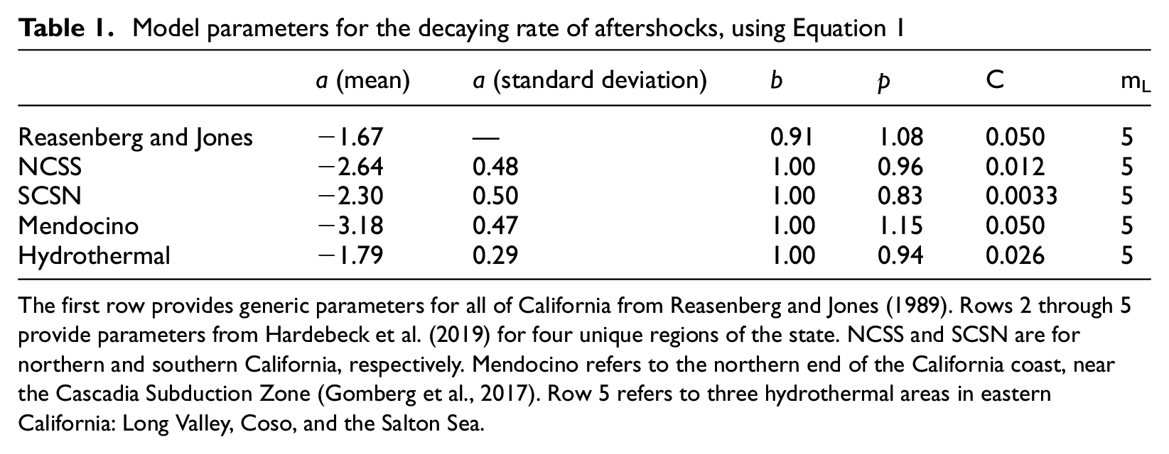
The first row provides generic parameters for all of California from Reasenberg and Jones (1989). Rows 2 through 5 provide parameters from Hardebeck et al. (2019) for four unique regions of the state. NCSS and SCSN are for northern and southern California, respectively. Mendocino refers to the northern end of the California coast, near the Cascadia Subduction Zone (Gomberg et al., 2017). Row 5 refers to three hydrothermal areas in eastern California: Long Valley, Coso, and the Salton Sea.

The case study presented here will use the Table 1 parameters for northern California (NCSS). Note that NCSS parameters reflect a less active aftershock environment than southern California (SCSN). The Hardebeck et al. (2019) parameters for each region are derived based on statistics and do not have direct physical meaning. However, the resulting aftershock occurrence intervals are consistent with intuition based on general knowledge of California’s fault geometries.

Step 2: aftershock hazard model

The Reasenberg and Jones (1989) model in Equation 1 is generally considered a reasonable approach for estimating the rate of aftershock events. However, engineers and decision-makers need the exceedance rate of specific shaking intensities, considering both aftershocks and steady-state events. The APSHA framework is a tool to quantify the rate of the former. This framework is described by Equations 2 and 3, which is conceptually similar to the more traditional PSHA model for the steady-state hazard (Cornell, 1968):

P (IM > im | Aftershock) = \int_{R} \int_{m_{l}}^{m_{m}} P (IM > im | m, r) f_{R | M} (r | m) f_{M} (m | m_{m}) dmdr

(2)

\begin{matrix} λ_{μ} (im, t, Δ t | m_{m}) = \int_{t}^{t + Δ t} μ (τ | m_{m}) d τ P (IM > im | Aftershock) \end{matrix}

(3)

The double integral (Equation 2) is familiar from PSHA (shown later by Equation 11), where $P (IM > im | m, r)$ is the probability of exceeding a shaking intensity, $im$ , given a rupture event of magnitude $m$ , with a site-to-rupture distance, $r$ . The probability density functions, $f_{R | M} (r | m)$ and $f_{M} (m | m_{m})$ , represent the distribution of possible aftershock locations and magnitudes, respectively. This equation provides the probability of exceedance given that an aftershock occurs, $P (IM > im | Aftershock)$ , by integrating over all possible aftershock locations and magnitudes. The integral term of Equation 3 provides the rate of aftershock occurrence over the time interval of interest $(Δ t)$ . Equation 3 provides the rate of exceeding a ground shaking intensity due to an aftershock, $λ_{μ}$ . This rate is conditioned on the mainshock magnitude, $m_{m}$ , and is computed over a specified duration $(Δ t)$ interval; and it depends on the intensity level $(im)$ and the number of days after the mainshock $(t)$ . Each term is discussed in more detail as follows.

Step 2.1: ground motion model

The ground motion hazard formulation of the APHSA model (Equation 3) is identical to the traditional steady-state PSHA model (discussed later in Equation 11), where $P (IM > im | m, r)$ is the probability of exceeding a shaking intensity, $im$ , given a rupture event of magnitude $m$ , with a site-to-rupture distance, $r$ . Any number of ground motion models (GMMs) could be used to describe the probability distribution for $P (IM > im | m, r)$ .

The case study uses the GMM by Boore et al. (2014, hereafter BSSA14), which is one of the models that is used for PSHA of the Western United States and has been recently validated for continued use (McNamara et al., 2020). The selected site in downtown San Francisco has an average shear wave velocity over the top 30 m of $V_{s 30} = 550 m / s$ , and the fault is assumed to be a vertical strike-slip with ruptures that reach the surface. The vertical strike-slip assumption is consistent with the faults that dominate the hazard in the San Francisco Bay Area. The BSSA14 GMM uses the Joyner–Boore distance (the closest distance to the surface projection of the fault plane, $R_{jb} = 13 km$ ) and does not include the depth to the top of the rupture, $Z_{tor}$ . As such, there is no sensitivity to the assumption that the rupture reaches the surface.

Recent studies (e.g. Shokrabadi et al., 2018) have suggested using GMMs, such as Chiou and Youngs (2008), which include significant differences in the spectral shape of the mainshock and aftershock ground motions. Note that use of a GMM that differentiates between mainshocks and aftershocks would also necessitate an aftershock-specific collapse fragility, due to the influence of the spectral shape on structural response. In contrast, the BSSA14 GMM used in the case study does not include spectral shape differences for aftershock events. Included with this article is a supplemental document with details of a sensitivity analysis to examine the aftershock hazard adjustment in Chiou and Youngs (2008) GMM. Selecting the GMM is an important assumption in the framework that must be carefully considered. Ideally, an implementation of this framework for decision-making in the public sector would consider the epistemic uncertainty in the selection of GMM via logic trees. Please note that defining such logic trees for an aftershock environment is outside the scope of this article.

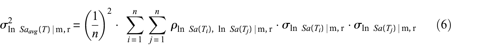
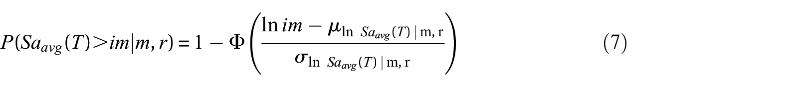
The choice of intensity measure, $im$ , used to quantify the level of shaking is another important consideration. The spectral acceleration, $Sa (T)$ , only accounts for the intensity at the fundamental period, $T$ , which tends to over-constrain the intensity measure for multi-degree-of-freedom structures and induce bias in collapse risk assessments. The dependence on a single period also increases the influence of spectral shape when assessing the collapse response. Using a GMM that changes the spectral shape of the aftershock hazard (e.g. Chiou and Youngs, 2008) would complicate the aftershock risk assessment, since one would need to develop separate collapse fragility curves for the spectral shapes of the mainshock and aftershock hazards. The average spectral acceleration, $S a_{avg} (T)$ defined in Equation 4, is an alternative intensity measure indexed over a wider range of periods (Eads et al., 2015) that helps overcome these limitations. The term “average” refers to the geometric mean of spectral values, or the log-average, calculated for $n$ linearly spaced periods (at 0.01-s intervals) over the range between $0.2 T$ and $3.0 T$ , as defined by Eads et al. (2015):

\ln S a_{avg} (T) = (\frac{1}{n}) \sum_{i = 1}^{n} \ln Sa (T_{i}), where 0.2 T \leq T_{i} \leq 3.0 T

(4)

An $S a_{avg} (T)$ GMM can be developed from traditional $Sa (T)$ GMMs by computing a predicted mean and variance using Equations 5 and 6 (Cordova et al., 2000; Kohrangi et al., 2016):

μ_{\ln S a_{avg} (T) | m, r} = (\frac{1}{n}) \cdot \sum_{i = 1}^{n} μ_{\ln Sa (T_{i}) | m, r}

(5)

σ_{\ln S a_{avg} (T) | m, r}^{2} = {(\frac{1}{n})}^{2} \cdot \sum_{i = 1}^{n} \sum_{j = 1}^{n} ρ_{\ln Sa (T_{i}), \ln Sa (T_{j}) | m, r} \cdot σ_{\ln Sa (T_{i}) | m, r} \cdot σ_{\ln Sa (T_{j}) | m, r}

(6)

$μ_{\ln Sa (T_{i}) | m, r}$ and $σ_{\ln Sa (T_{i}) | m, r}$ are the predicted log mean and standard deviation of $Sa (T_{i})$ for all $n$ periods, $T_{i}$ , that span the range $0.2 T \leq T \leq 3 T$ , and $ρ_{\ln S a (T_{i}), \ln S a (T_{j}) | m, r}$ is the correlation between $\ln Sa$ values at periods $T_{i}$ , and $T_{j}$ , quantified by Baker and Jayaram (2008). Assuming that $S a_{avg} (T)$ follows a lognormal distribution, $P (IM > im | m, r)$ is calculated using the standard normal cumulative distribution function as per Equation 7:

P (S a_{avg} (T) > im | m, r) = 1 - Φ (\frac{\ln im - μ_{\ln S a_{avg} (T) | m, r}}{σ_{\ln S a_{avg} (T) | m, r}})

(7)

Step 2.2: aftershock event distribution

The event distribution terms, $f_{M} (m | m_{m})$ and $f_{R | M} (r | m)$ , represent the likelihood of occurrence for an aftershock of a given magnitude, $m$ , and site-to-rupture distance, $r$ . As discussed above, these aftershock parameters feed directly into the ground motion equation.

The aftershock magnitude distribution is based on the bounded Gutenberg–Richter recurrence law re-written in Equation 8 (Cornell and Vanmarcke, 1969):

f_{M} (m) = \frac{β e^{- β (m - m_{l})}}{1 - e^{- β (m_{u} - m_{l})}}, β = b \cdot \ln 10, m_{l} < m \leq m_{u}

(8)

where $b$ is the Gutenberg–Richter value for the site, and $m_{u}$ is the upper bound for the possible magnitudes (all other terms were introduced with Equation 1). The lower bound is taken as $m_{l} = 5$ , in keeping with Table 1 and the common PSHA assumption that $m < 5$ would not cause damage to engineered buildings. This study assumes that the maximum possible aftershock magnitude, $m_{u}$ , is equal to the mainshock magnitude, $m_{m}$ , as in the work by Yeo and Cornell (2009). In this way, the aftershock magnitude distribution is conditioned on the mainshock magnitude, $f_{M} (m | m_{m})$ . To facilitate the visualization of this $m_{u} = m_{m}$ upper bound on the aftershock magnitude, Equation 9 presents the cumulative probability distribution of aftershock magnitudes by integrating Equation 8. Figure 3a shows Equation 9 for three values of $m_{u}$ , where each curve terminates with a vertical asymptote at $m_{m}$ . The convergence of the three curves at the vertical dotted line in Figure 3a indicates that the three mainshocks all have a $~ 10 %$ probability of an aftershock exceeding $m = 6$ :

G_{M} (m | m_{m}) = 1 - F_{M} (m | m_{m}) = 1 - \frac{1 - 10^{- b (m - m_{l})}}{1 - 10^{- b (m_{m} - m_{l})}}, m_{l} < m \leq m_{m}

(9)

Figure 3.

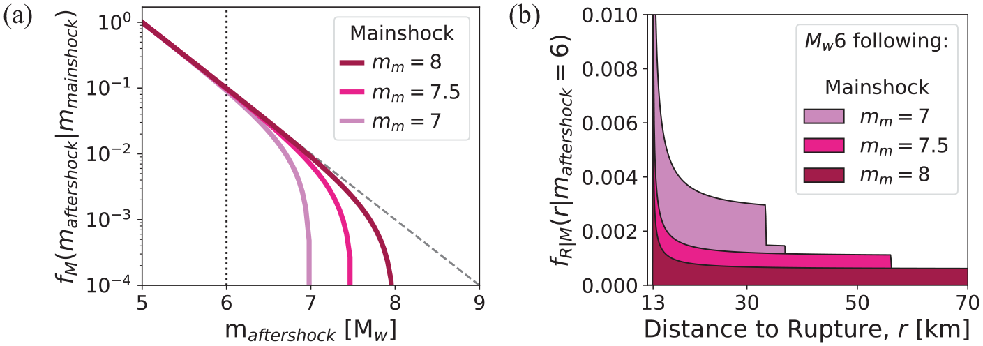
Aftershock event distributions: (a) Magnitude: the probability of exceedance for the Gutenberg–Richter recurrence law, bounded by the magnitude of each mainshock event. The vertical dotted line crosses at the probability of an aftershock magnitude $m > 6$ , given that an aftershock occurs ( $~ 10 %$ for each mainshock magnitude); (b) location: the probability distribution of distances from a $m = 6$ aftershock rupture to the site. The range of possible distances depends on the length of the mainshock rupture (the maximum distance following a $m_{m} = 8$ mainshock is almost 200 km, too far to include in the figure).

The aftershock location distribution is conditioned on the magnitude, as implied by the $f_{R | M} (r | m)$ term. This case study follows Yeo and Cornell’s (2009) model of uniformly distributing the possible locations of aftershocks along the length of the mainshock rupture. The length of the aftershock rupture is based on the Wells and Coppersmith (1994) relationship for strike-slip faults, $\log (L) = 0.74 M_{w} - 3.55$ , where $M_{w}$ is the magnitude and $L$ is the surface rupture length. While the case study does not consider uncertainty on these coefficients, the sensitivity to this assumption is discussed below (also see the supplemental document for more details). In this study, the length of the aftershock rupture is fixed for a given magnitude (e.g. $m = 6$ ), such that the location distribution of the aftershock rupture depends only on the geometry of the mainshock Figure 3b illustrates the distribution of rupture distances given magnitude, $f_{R | M} (r | m)$ , where the longer rupture lengths associated with higher mainshock magnitudes increase the range of possible distances from the site to the rupture, $r$ , stretching the distribution horizontally. The steps at the end of the $f_{R | M} (r | m)$ distributions reflect the mainshock rupture geometries, which are not quite symmetric with respect to the case study site.

Step 2.3: rate of aftershock occurrence

The rate of aftershock occurrence term, $μ (t, Δ t | m_{m})$ , refers to the mean rate of aftershocks following a mainshock magnitude, $m_{m}$ , during a time window of interest, $τ$ , starting at time $t$ and lasting $Δ t$ days. The amount of daily rate decay depends on the specified duration, $Δ t$ . Yeo and Cornell (2009) integrated Equation 1 to transform the rate of aftershocks from a time interval of 1 day (daily rate) into an interval of an arbitrary duration, $Δ t$ (Equation 10):

\begin{matrix} μ (t, Δ t | m_{m}) = \int_{t}^{t + Δ t} μ (τ | m_{m}) d τ \\ = \frac{10^{a + b (m_{m} - m_{l})} - 10^{a}}{p - 1} [{(t + c)}^{1 - p} - {(t + Δ t + c)}^{1 - p}] \end{matrix}

(10)

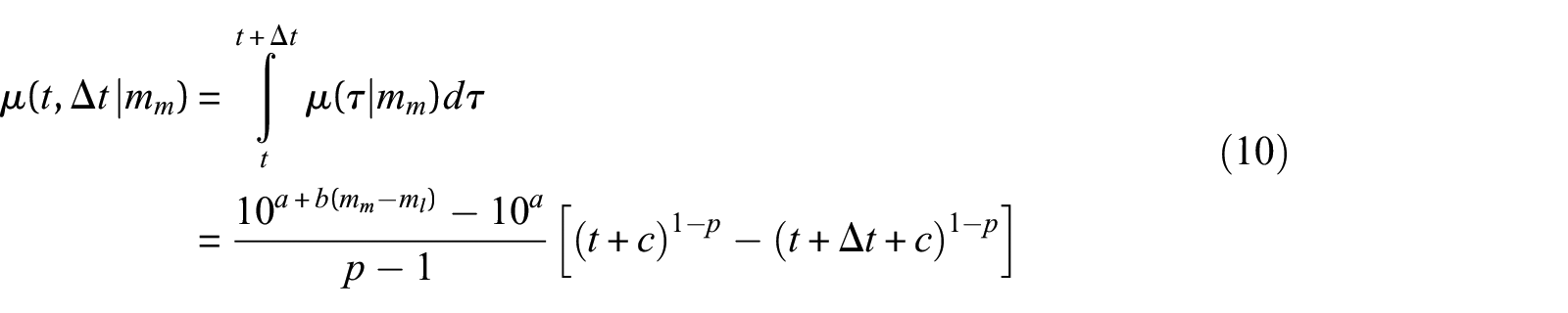
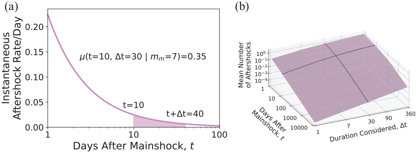
The parameters in Equation 10 were defined in Table 1. Assuming the NCSS values for a generic northern California aftershock environment, the decay in the daily rate of aftershocks following a $m_{m} = 7$ mainshock is shown in Figure 4a. While the case study uses the mean value for $a$ , the sensitivity to this assumption is discussed below (see the supplemental document for more details). Using Equation 10 with the rates in Figure 4a, one can draw a surface for the mean number of aftershocks as a function of the start date, $t$ , and the duration considered, $Δ t$ (Figure 4b). Assuming a time window, $τ$ , starting on the 10th day and spanning $Δ t = 30$ days, the mean number of aftershocks during $τ$ is 0.35. The rate can be considered a mean monthly exceedance frequency when calculated over $Δ t = 30$ days.

Figure 4.

The rate of aftershocks over time (Equation 10): (a) The purple line shows the daily rate of aftershocks following a $m_{m} = 7$ mainshock, as the rate decays over time. Integrating from $t$ to $t + Δ t$ (the shaded area) provides the mean number of aftershocks that will occur during that time window; (b) mean number of aftershocks following a $m_{m} = 7$ mainshock, as a function of the start time, $t$ , and duration considered, $Δ t$ , produces a surface. The black lines cross at 0.35 aftershocks for $t = 10$ days and $Δ t = 30$ days, from (a).

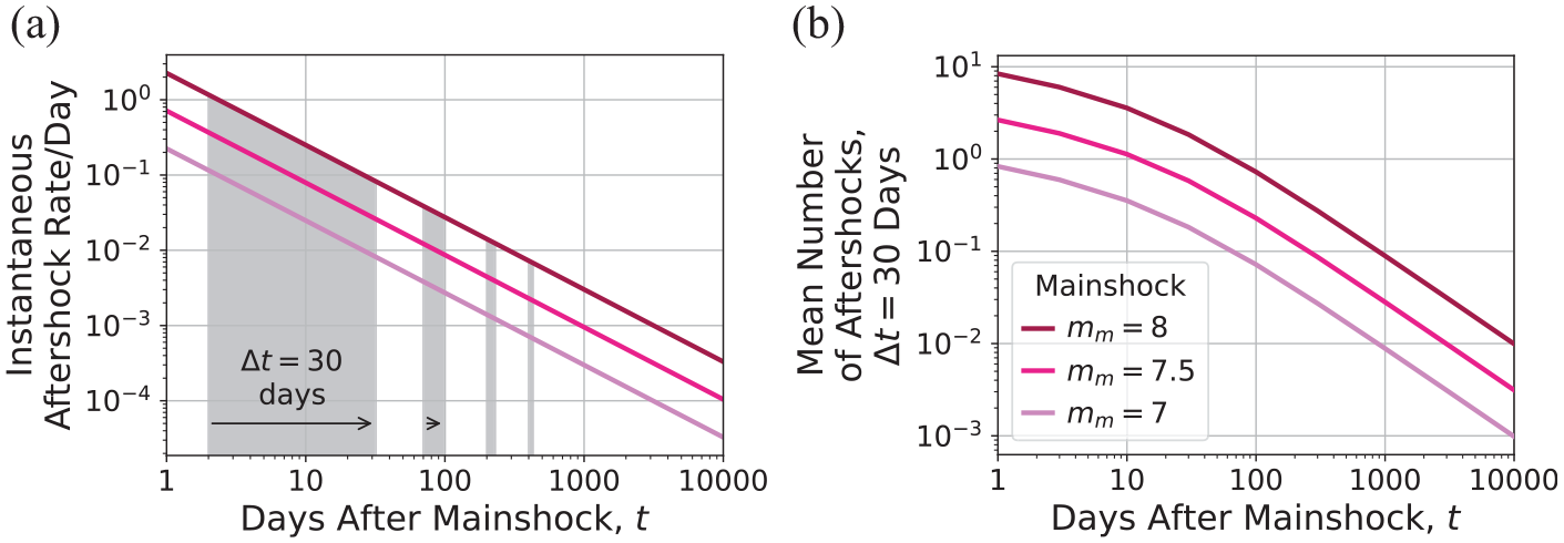
The vertical axis in Figure 4b is in log scale, making the exponential decay rate appears linear for $Δ t = 1$ day. This linear trend in log scale also appears in Figure 5a, which shows the daily rate for all three mainshock magnitudes. The gray bands reveal the effect of the time axis’s log scale, such that the same month-long duration, $Δ t$ , shrinks as the start time, $t$ , increases. Integrating over a constant $Δ t$ for increasing start times, $t$ , produces a mean number of aftershock curves that are no longer linear in log scale (Figure 5b). The duration of interest depends on the type of decisions the study will inform (see the supplemental document for the sensitivity to this assumption).

Figure 5.

The rate of aftershocks (Equation 10) following each mainshock event: (a) The daily rate of aftershocks is linear in log scale. The gray bands visually depict the effect of the log scale, which appears to shrink the constant width of the duration, $Δ t = 30$ days, as the start time, $t$ , increases; (b) using a constant $Δ t = 30$ with increasing start times produces mean number of aftershock curves that are not linear in log scale.

The magnitude and location distributions provide the input needed for the GMM. Integrating over all possible aftershock events (Equation 2) provides the probability of exceeding a shaking intensity given that an aftershock occurs, $P (IM > im | Aftershock)$ . With all terms of the APSHA model defined, Equation 3 calculates the time-dependent hazard due to aftershock events, $λ_{μ} (im, t, Δ t | m_{m})$ . This aftershock portion of the hazard must then be combined with the steady-state hazard to obtain the full seismic hazard at the site.

Step 3: elevated hazard curve

The APSHA framework only considers the elevated and decaying hazard within a single earthquake cluster. To obtain the total seismic hazard in an aftershock environment, one needs to combine the aftershock with the steady-state earthquake rates, resulting in a hazard that is elevated after a mainshock but decays back to a steady state over time.

Both PSHA and APSHA calculate the rate of exceeding a shaking intensity, $im$ , based on the rate of event occurrence and the probability of exceeding the shaking intensity, given that an event occurred, $P (IM > im | Event)$ . For APSHA, Equation 3 is the governing equation as discussed in the previous section. Similarly, Equation 11 is the governing equation for PSHA. Recall that Equation 3 relies on the same concepts as Equation 11 but has a time-dependent rate of occurrence, and the event distribution is conditioned on the mainshock:

λ_{ν} (im, Δ t) = ν (Δ t) \int_{R} \int_{m_{l}}^{m_{u}} P (IM > im | m, r) f_{R | M} (r | m) f_{M} (m) dmdr

(11)

In Equation 11, $ν (Δ t)$ is the estimated number of steady-state mainshock occurrences over the duration $Δ t$ . This term is equivalent to the rate of aftershock occurrence, $μ (t, Δ t | m_{m})$ , but is constant instead of being conditioned on a recent event. The upper limit of magnitude, $m_{u}$ , depends on fault geometry (in contrast to the aftershock case, where $m_{u}$ is assumed to equal the mainshock magnitude).

Figure 6a illustrates the $P (IM > im | Event)$ calculation for aftershock events following each of the three considered mainshock events $(m_{m} = 7, 7.5, and 8)$ . Note that the probability of exceeding smaller values of $im$ during an aftershock is larger for the $m_{m} = 7 and 7.5$ mainshocks compared with the $m_{m} = 8.0$ mainshock, with the curves converging here $0.4 g$ . This is the consequence of assuming that the mainshocks occur on the portion of the fault nearest to downtown San Francisco and that aftershocks are confined to the mainshock rupture length (per Yeo and Cornell, 2009). With this assumption, the mainshocks’ longer rupture lengths result in the potential for small magnitude aftershocks to occur further away from downtown San Francisco. On the contrary, the higher mainshocks have a larger rupture plane available to produce stronger magnitude aftershocks, increasing the probability of large $im$ values compared with smaller magnitude mainshocks. Note that the lines that converge in Figure 6a are parallel in Figure 6b, due to the additional term for the rate of aftershock occurrence. This figure shows the combined aftershock hazard curve for a range of intensities, $im$ , considering the 1-month duration, starting 10 days after each mainshock, $λ_{μ} (t = 10, Δ t = 30)$ (note that $λ (im)$ refers to the rate of exceeding a single value of $im$ , while $λ$ refers to the whole hazard curve).

Figure 6.

$λ_{μ} (im) : Rate of IM > im$ due to an aftershock: (a) $P (IM > im | Aftershock)$ : The probability of exceeding a range of $Sa (2.3)$ intensities, $im$ , given the occurrence of an aftershock (of any magnitude and location); (b) $λ_{μ} (im) = μ (t, Δ t | m_{m}) \times P (IM > im | Aftershock)$ : The higher rate of aftershock occurrence for larger mainshock magnitudes differentiates the aftershock hazard curves for $Sa (2.3)$ .

To obtain the steady-state hazard curve, this case study integrates over all mainshock events by using SimCenter’s EQHazard tool (available at https://github.com/NHERI-SimCenter/GroundMotionUtilities/tree/master/EQHazard https://github.com/NHERI-SimCenter/GroundMotionUtilities/tree/master/EQHazard) to compile an event catalog from OpenSHA’s Monte Carlo event set for UCERF2 Field et al. (2008). The catalog includes all events within a 200-km radius of downtown San Francisco. The events are then sorted into discrete magnitude and distance bins $(dm = 0.25 M_{w}, dr = 10 km)$ with an annual rate of occurrence for each bin, $ν (Δ t = 365 days)$ . The $ν (Δ t) \int_{R} \int_{m_{l}}^{m_{u}} f_{R | M} (r | m) f_{M} (m) dmdr$ terms in Equation 11 can be sorted into paired bins such that $P (IM > im | m, r)$ can be assessed for each $m, r$ bin. For simplicity, the case study assumes the same rupture parameters for all events: a vertical strike-slip fault with a surface rupture (the same assumption used for the aftershock events). Finally, the annual rate of exceedance, $λ_{ν} (im, Δ t = 365)$ , is scaled to the 1-month rate of exceedance, $λ_{ν} (im, Δ t = 30)$ . Computing the hazard curve in this way enables incorporating any ground motion exceedance equation, including Equation 7 for $S a_{avg} (T)$ .

Both the aftershock $(λ_{μ})$ and steady-state $(λ_{ν})$ hazard curves contribute to the elevated hazard curve $(λ_{π})$ , which is conditioned on the mainshock, $m_{m}$ , and decays over time, $t$ . The elevated hazard is the sum of the respective rates of exceedance, $λ (im)$ , for a range of intensities (Equation 12):

λ_{π} (im, t, Δ t | m_{m}) = λ_{μ} (im, t, Δ t | m_{m}) + λ_{ν} (im, Δ t)

(12)

Figure 7a shows the hazard following a $m_{m} = 7$ mainshock (the hazard curve is on the $Sa (T) axis$ ) as it decays through time, $t$ (the days after mainshock axis). Depending on the time, $t$ , the elevated hazard ( $λ_{π}$ , dark purple with solid lines) may be dominated by the aftershock hazard ( $λ_{μ}$ , light purple with dotted lines) or the steady-state hazard ( $λ_{ν}$ , black with dashed lines). The plots of hazard curves for $t = 10$ days after each mainshock, shown in Figure 7b, reveal that the relative contribution of the aftershock versus steady-state rates of exceedance, $λ (im)$ , varies across the range of shaking intensities, $im$ . Ten days after a $m_{m} = 7$ mainshock, the lower intensities $(0.001 g \leq Sa (2.3) \leq 0.1 g)$ are dominated by the aftershock hazard. The aftershock and steady-state hazard contributions converge around $Sa (2.3) = 0.3 g$ . This trend of the aftershock contribution decreasing for higher intensities is most apparent 300 days after the $m_{m} = 7$ and 7.5 mainshocks (Figure 7c), where the decaying contribution of the aftershocks falls below that of the steady-state hazard for $Sa (2.3) > 0.03 g$ . This is because only large-magnitude events can produce high $Sa (2.3)$ intensities. As the upper bound on aftershock magnitudes increases with the mainshock magnitude $(m_{u} = m_{m})$ , only large mainshocks can generate the large aftershocks associated with high $im$ values.

Figure 7.

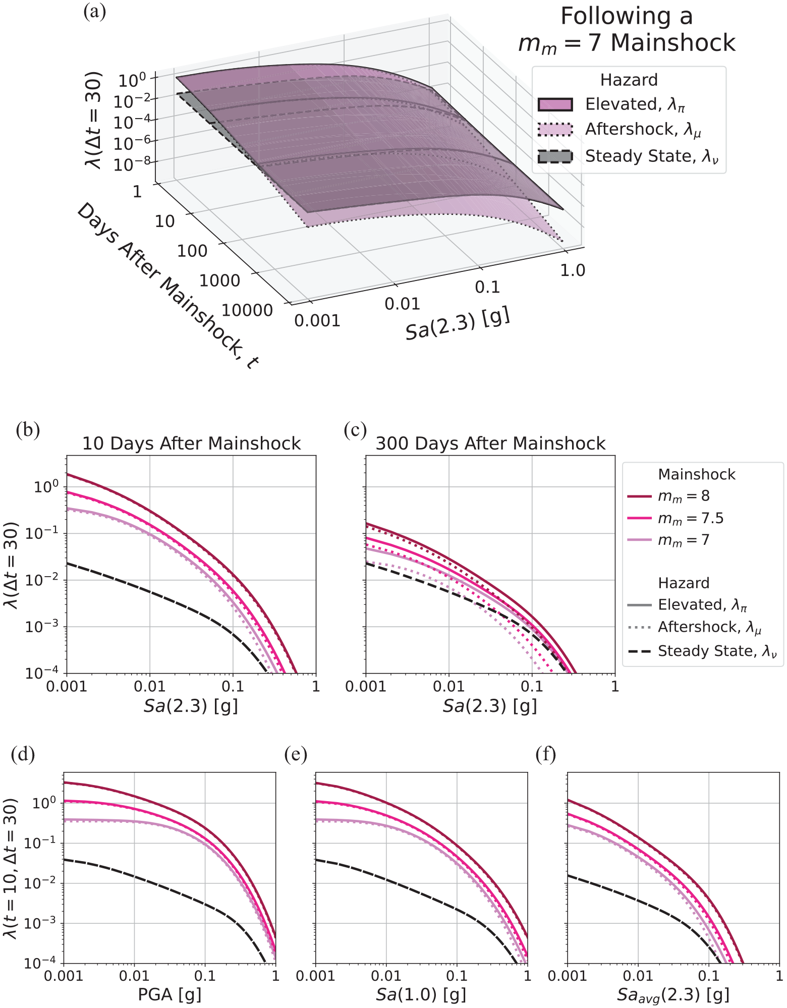
The elevated hazard includes both the aftershock and steady-state hazards: (a) $Sa (2.3)$ hazards following a $m_{m} = 7$ mainshock. The aftershock hazard (light purple) decays over time. The steady-state hazard (black) remains constant. The elevated hazard (dark purple) is the sum of the two. Each surface is marked at $t = 10$ and 300 days; (b) the hazard curves after 10 days, for each mainshock event; (c) after 300 days; (d) $PGA$ after 10 days; (e) $Sa (1.0)$ ; (f) $S a_{avg} (2.3)$ .

Figure 7d, e, and f shows the $t = 10$ day hazard curves for three intensity measures: peak ground acceleration $(PGA)$ , $Sa (1.0)$ , and $S a_{avg} (2.3)$ , respectively. In contrast to the results shown for $Sa (2.3)$ in Figure 7b, the aftershock hazard for $PGA$ is equal to or greater than the steady-state hazard for all intensities, even following the $m_{m} = 7$ event. This is because even low-magnitude events can generate high intensities at the high frequencies inherent in $PGA$ . For $Sa (1.0)$ and $S a_{avg} (2.3)$ following the $m_{m} = 7$ mainshock, the relative contributions due to aftershocks converge to the steady-state hazard at high intensities, similar to $Sa (2.3)$ .

Collapse risk for an individual building

With the elevated hazard model (M1 in Figure 1) complete, the next modules address the damaged building performance (M2) and the elevated risk (M3). These modules are illustrated with an individual building in this section and with a range of generic buildings (i.e. a parametric study) in the following section. Building collapse risk is calculated by integrating the ground motion hazard and the building’s collapse fragility. Since the ground motion hazard is described in terms of a temporal rate, the risk of building collapse under earthquakes is likewise typically expressed as a rate of collapse, $λ_{collapse}$ , which can be calculated as shown in Equation 13 (Krawinkler et al., 2006):

λ_{collapse} = \int_{IM} P (C | im) | d λ_{IM} (im) |

(13)

where $P (C | im)$ is the probability of collapse at the shaking intensity (the collapse fragility curve) and $λ_{IM} (im)$ is the rate of exceeding any shaking intensity, $IM$ , which could be evaluated for the combined, only aftershock, or only steady-state hazards, $λ_{π}, λ_{μ}, and λ_{ν}$ , respectively. The rate of collapse will inherit the time interval used for the hazard exceedance curve, which for the aftershock studies is treated as the mean monthly $(Δ t = 30)$ rate of exceedance. One can consider the risk of collapse in terms of the rate itself, $λ_{collapse}$ , or in terms of a probability of collapse over a specified time interval, for example, X% probability of collapse in Y days.

Damaged building collapse fragilities (module 2)

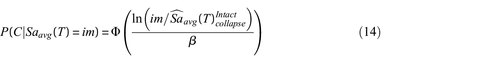
The collapse risk after a mainshock depends on the intact building’s collapse fragility (the probability of collapse as a function of the earthquake shaking intensity), as well as any damage the building may have experienced during the mainshock. In contrast to the conventional fragility function, $P (C | im)$ , when evaluating postearthquake risk, the collapse fragility is conditioned on an intensity measure, $IM$ , and a damage metric, $DI : P (C | im, di)$ . The predictive power of the collapse fragility depends on the choice of $IM$ and $DI$ .

Concerning the choice of $IM$ , Eads et al. (2015), Kohrangi et al. (2016), and others have shown that average spectral acceleration, $S a_{avg} (T)$ , is less sensitive to record selection than $Sa (T)$ (Jayaram et al., 2011; Lin et al., 2013) for collapse estimation. This is because $S a_{avg} (T)$ accounts for the spectral shape over a range of periods $(0.2 T \leq T \leq 3 T)$ , rather than only considering the intact building’s fundamental period, $T$ . This feature is particularly useful in differentiating between the probability of collapse for a damaged versus intact buildings, given that the damage will elongate the period with respect to that of the intact building.

Galvis et al. (2023) propose a methodology for estimating the collapse safety of a damaged building, based on $S a_{avg} (T)$ to characterize the earthquake shaking. First, the intact building is subjected to an incremental dynamic analysis (IDA) (Vamvatsikos and Cornell, 2002) for a specified set of ground motions. The use of ${\hat{Sa}}_{avg} (T)$ as the intensity measure reduces the resulting fragilities’ dependence on the specific set of ground motions (Eads et al., 2015), as well as the sensitivity to scale factor bias (Davalos, 2018). For the fragility curves used in this study, Galvis et al. (2023) applied the FEMA P695 ground motions “back-to-back” to calculate the intact and damaged collapse fragilities (FEMA, 2009). The collapse limit state was quantified as a story drift ratio exceeding 10% or a slope of the IDA curve less than 20% of the elastic slope of the curve (Vamvatsikos and Cornell, 2004). These IDA results are used to fit a lognormal collapse fragility (Equation 14) with two parameters: a median collapse intensity, ${\hat{Sa}}_{avg} (T)_{collapse}^{Intact}$ , and a standard deviation, $β_{RTR}$ , using the maximum likelihood estimation approach described by Baker (2015). Galvis et al. (2023) demonstrated that the level of damage does not significantly affect $β_{RTR}$ . Since $β_{RTR}$ only captures the record-to-record variability of the collapse shaking intensity, the total dispersion of the collapse fragility, $β$ , is increased by the uncertainty in the design requirements $(β_{DR})$ , the uncertainty in test data $(β_{TD})$ , and the uncertainty in the robustness of the models $(β_{MDL})$ using Equation 15. The values of $β_{DR}$ , $β_{TD}$ , and $β_{MDL}$ are selected following the guidelines in FEMA P695:

P (C | S a_{avg} (T) = im) = Φ (\frac{\ln (im / {\hat{Sa}}_{avg} (T)_{collapse}^{Intact})}{β})

(14)

β = \sqrt{β_{RTR}^{2} + β_{DR}^{2} + β_{TD}^{2} + β_{MDL}^{2}}

(15)

Next, the intact building is subjected to each of the ground motion records, scaled to multiple intensities, to induce different levels of damage that may occur under an earthquake mainshock. Each of these analyses is considered a building damage instance, which is described by a scalar DI calculated as a function of one or more structural demand parameters (e.g. peak story drift) under the damaging ground motion. Then, a second IDA is performed, using the same set of ground motions as applied to the intact building, to determine the median collapse capacity of the damaged building, ${\hat{Sa}}_{avg} (T)_{collapse}^{Damaged}$ . The median collapse capacity for each damage instance is then normalized by the intact median to define $κ$ (Equation 16):

Fraction of {\hat{Sa}}_{collapse}^{Intact}, κ = \frac{{\hat{Sa}}_{avg} (T)_{collapse}^{Damaged}}{{\hat{Sa}}_{avg} (T)_{collapse}^{Intact}}

(16)

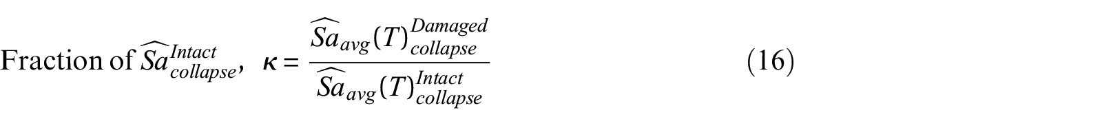
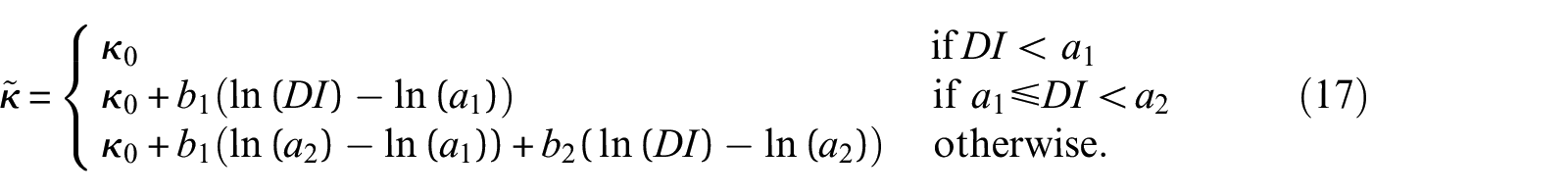
The purpose of simulating damage instances and assessing their new collapse performance is to fit a regression for $κ$ based on the scalar DIs. Galvis et al. (2023) propose the trilinear expression in Equation 17 to relate $DI$ to $κ$ :

\tilde{κ} = {\begin{matrix} κ_{0} if DI < a_{1} \\ κ_{0} + b_{1} (\ln (DI) - \ln (a_{1})) if a_{1} \leq DI < a_{2} \\ κ_{0} + b_{1} (\ln (a_{2}) - \ln (a_{1})) + b_{2} (\ln (DI) - \ln (a_{2})) otherwise . \end{matrix}

(17)

Galvis et al. (2023) assessed the damaged collapse fragilities for ductile reinforced concrete (RC) moment frames designed per ASCE 7-02 (2002) and ACI 318-05 (2005) for a high seismic hazard location in Los Angeles on soil class D. The archetype designs and numerical models were developed by Haselton et al. (2008). The archetypes were idealized as two-dimensional frames and modeled using OpenSees where beam and column hinges are lumped plasticity elements using the Ibarra-Medina-Krawinkler (IMK) model (Ibarra et al., 2005) with parameters specifically calibrated for RC elements. The flexibility of beam-column joints is represented by an elastic spring implemented by the Joint2D (Altoontash, 2004) element in OpenSees. The column bases have elastic rotational springs to represent foundation flexibility. The destabilizing effects of the gravity framing are included by means of a leaning column.

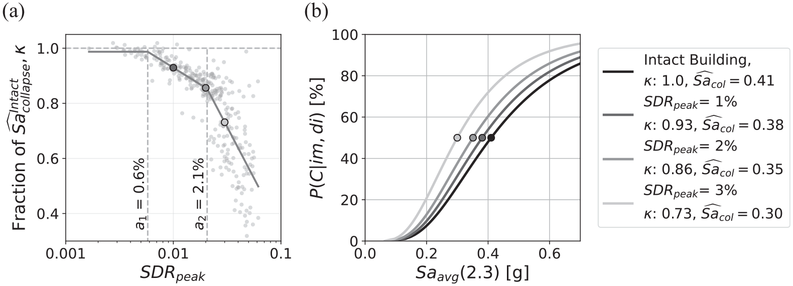
The case study focuses on a 20-story building with $T = 2.3$ s and ${\hat{Sa}}_{avg} (T)_{collapse}^{Intact} = 0.41 g$ (see the supplemental document for additional data on 8- and 4-story buildings). Figure 8a shows the trilinear regression model for the damage instances, where the $DI$ is defined as the peak story drift ratio, $SD R_{peak}$ . The equation parameters are as follows: $κ_{0} = 0.99, a_{1} = 0.6 %, b_{1} = - 0.11, a_{2} = 2.1 %, b_{1} = - 0.32$ . The larger circles on the trilinear trend line denote the predicted $κ$ values for $S D R_{p e a k} = 1 %, 2 %, 3 %$ . Note that after the $a_{2}$ threshold at $S D R_{p e a k} = 2.1 %$ , the building stability is compromised, resulting in a steeper slope for $κ$ . Figure 8b shows the same $κ$ values, now plotted as fragilities with ${\hat{Sa}}_{col} : {\hat{Sa}}_{avg} (T)_{collapse}^{Damaged} = κ \times {\hat{Sa}}_{avg} (T)_{collapse}^{Intact} .$

Figure 8.

Collapse performance of a damaged 20-story, modern reinforced concrete frame building: (a) The median collapse intensity (quantified with $κ$ ) decreases as the mainshock $SD R_{peak}$ increases. The larger circles denote the predicted $κ$ values for $S D R_{p e a k} = 1 %, 2 %, 3 %$ , based on the trend line (Equation 17); (b) the reduced $κ$ values correspond to a leftward shift in the collapse fragility curves. The shaking intensity is the average spectral acceleration at the building’s fundamental period, $S a_{avg} (2.3)$ (see Galvis et al. (2023) for more details).

Elevated collapse risk (module 3)

Using the elevated hazard curves and the collapse fragilities of a damaged building, the collapse risk for each damage instance can be computed in terms of the rate of collapse, $λ_{collapse}$ , following Equation 13 using $λ_{π}$ and $P (C | im, di)$ . In keeping with the hazard calculations described previously, $λ_{collapse}$ is defined as the mean monthly rate of collapse (corresponding to $Δ t = 30$ $days$ in Equation 12). To help communicate the increase in collapse risk, a risk multiplier (RM) is defined as the rate of collapse over the steady-state rate of collapse, $λ_{collapse} / λ_{collapse}^{OriginalRisk}$ . The steady-state rate considers the intact building’s collapse fragility, $P (C | im)$ , and the steady-state hazard, $λ_{ν}$ .

Due to the aftershock hazard, the risk of collapse of any building increases compared with the steady state until the aftershock hazard decays to a negligible level. Figure 9a presents the effect of aftershocks for the intact 20-story building introduced in the previous section. Figure 9a considers the $S a_{avg} (2.3)$ hazard following the three mainshock magnitudes shown in Figure 7f. Consider a tagging criterion such that the building is deemed unsafe to reoccupy whether the $RM > 6$ , which is the safety threshold used by Yeo and Cornell (2004) for commercial and office buildings. Based on these assumptions, the intact 20-story building would be immediately occupiable after a $m_{m} = 7$ and 7.5 mainshock. By contrast, following a $m_{m} = 8$ mainshock, the same intact building would require $~ 40$ days to meet the $RM \leq 6$ criterion. This may suggest that, for practical reasons, one may need to consider higher RM thresholds for higher magnitude mainshocks. Nevertheless, the $6 \times λ_{collapse}^{Original Risk}$ threshold is useful for benchmarking and comparing the results.

Figure 9.

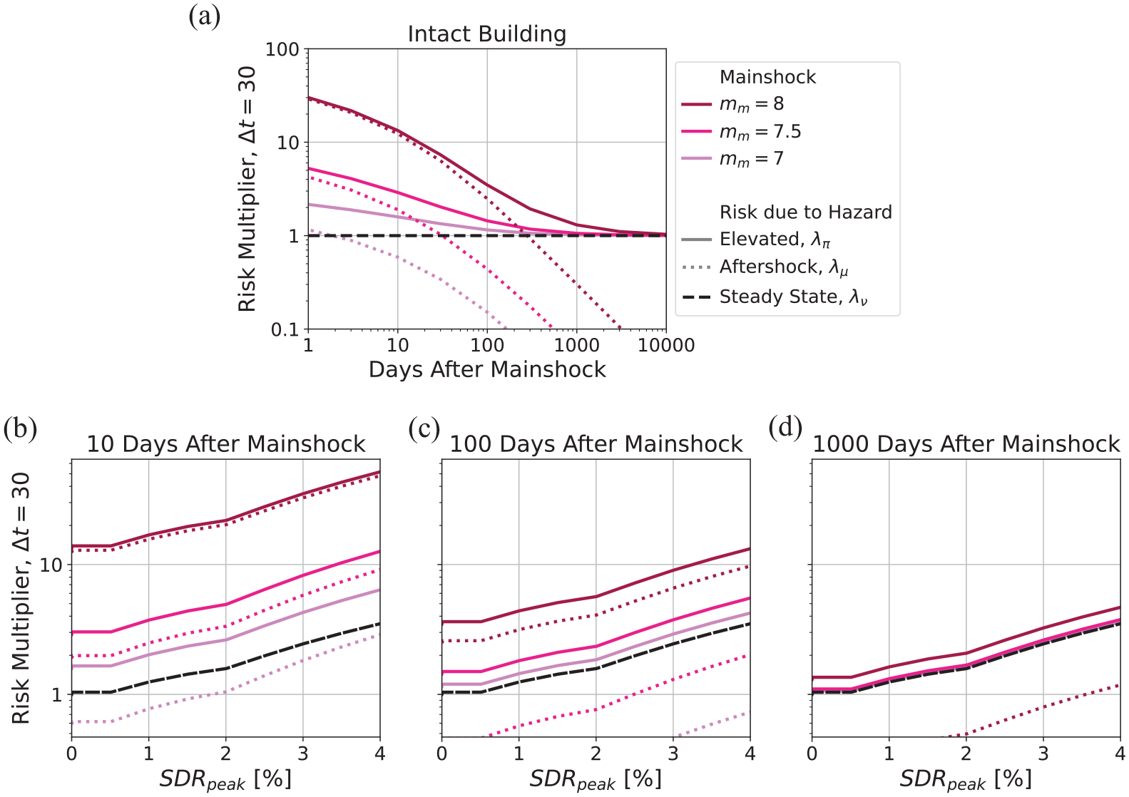
Elevated risk due to aftershocks and building damage: (a) The intact building’s risk multiplier following each mainshock magnitude decays over time. The solid, dotted, and dashed lines correspond to the $S a_{avg} (2.3)$ hazards: elevated, $λ_{π}$ , aftershock, $λ_{μ}$ , and steady state, $λ_{ν}$ , from Figure 7f; (b) the RMs at 10 days after the mainshock increase with building damage $(SD R_{peak})$ for all hazard sources (including the black dashed line for steady state, $λ_{ν}$ ); (c) 100 days; (d) 1000 days.

In addition to the change in risk due to elevated aftershock hazard, building damage caused by the mainshock will also increase the risk by reducing the collapse capacity, as indexed by $κ$ . Figure 9b shows the RMs, evaluated 10 days after each mainshock, for increasing levels of building damage, as measured by the peak drift demands $SD R_{peak}$ , caused by the mainshock. Following a $m_{m} = 7$ mainshock, any damage up to $S D R_{p e a k} = 4 %$ (the right edge of the figure) is theoretically below the RM threshold of 6. By the $100^{th}$ day after the $m_{m} = 8$ mainshock (Figure 9c), the RM still exceeds 6 for buildings that experience $S D R_{p e a k} > 2 %$ , though by 1000 days (3 years) the RM is below 6 even for $S D R_{p e a k} = 4 %$ . However, the risk increases more sharply with damage for $S D R_{p e a k} > 2 %$ , which corresponds to the damage threshold ( $a_{2}$ in Figure 8a) where the collapse capacity begins to drop off with a steeper slope. Due to the rapid decrease in collapse capacity past the damage threshold, Galvis et al. (2023) recommended that such buildings be red-tagged, even if their RM is below the tagging threshold.

Collapse risk for a parametric study

Communities are comprised of large inventories of buildings with varying heights, configurations, materials, and ages, which will affect their dynamic response and resistance to earthquake damage. To start moving beyond the individual building to community-scale earthquake risks, buildings with varying fundamental periods of vibration and design strengths (as implied by their inherent structural collapse capacities) are evaluated.

Damaged building collapse fragilities (module 2)

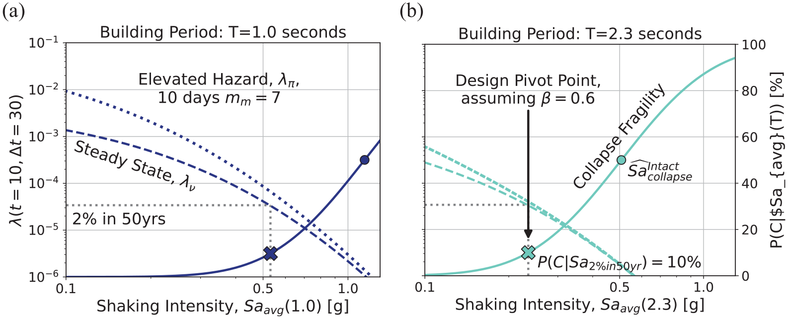
The first parameter considered is the building period. Figure 10a and b superimposes the collapse fragility curves and seismic hazard curves for two buildings with periods of $T = 1.0 and 2.3$ s, respectively. The left axes (corresponding to the seismic hazard curves) show the rate of exceeding a shaking intensity at $t = 10$ days after a $m_{m} 7$ mainshock $(Δ t = 30 days)$ , and the right axes (corresponding to the collapse fragility curves) show the probability of collapse, conditioned on $S a_{avg} (T)$ . The steady-state hazard curve ( $λ_{ν}$ , dashed line) is shown to help anchor the seismic design basis of the building, and the elevated hazard ( $λ_{π}$ , dotted line) includes the additional hazard due to aftershocks from a $m_{m} = 7$ mainshock.

Figure 10.

Examples of the parametric collapse fragilities that represent a building inventory, shown here for fundamental periods of $T = 1.0 and 2.3 s$ (dark blue and light green, respectively): (a) The design shaking intensity, $S a_{2 % in 50 yr}$ , is based on the steady-state hazard curve (dashed line). The elevated hazard (dotted line) is higher because of the additional contribution of aftershock ground motions, 10 days after a $m_{m} 7$ mainshock event; (b) the median collapse intensity for an intact building design ( ${\hat{Sa}}_{collapse}^{Intact}$ , circles) is back-calculated from the probability of collapse at the design shaking intensity, $P (C | S a_{2 % in 50 yr})$ (marked by Xs. In this example, = 10%), and the assumed collapse fragility dispersion $(β = 0.6)$ .

The collapse fragility curve is anchored to a 10% probability of collapse for a ground motion $S a_{avg} (T)$ with a probability of exceedance equal to 2% in 50 years per the steady-state hazard. This point is indicated by the X mark on the collapse fragility curve. This anchor point, $P (C | S a_{2 % in 50 yr}) = 10 %$ , is analogous to the nominal building code target (Luco et al., 2007), making the tacit assumption that the $S a_{2 % in 50 yr}$ hazard is equivalent to the risk-targeted maximum considered earthquake $(MC E_{R})$ design basis. The median collapse intensity for the collapse fragility of the intact building, ${\hat{Sa}}_{avg} (T)_{collapse}^{Intact}$ , is determined based on the anchor point and an assumed logarithmic standard deviation of $β = 0.6$ , which is consistent with the assumptions used to develop the risk-targeted $MC E_{R}$ ground motion hazard (Luco et al., 2015). In the parametric study, the anchor point $P (C | S a_{2 % in 50 yr})$ is adjusted vertically to represent buildings whose collapse capacities differ from the nominal building code target, $P (C | S a_{2 % in 50 yr}) = 10 %$ . An anchor point lower than 10% represents buildings designed to higher performance targets, while an anchor point with a higher probability represents more vulnerable buildings.

Once ${\hat{Sa}}_{collapse}^{Intact}$ is established for each building design, structural damage associated with mainshock earthquakes can be applied by adjusting the median value of the collapse fragility curve by $κ$ . As suggested in the work by Galvis et al. (2023), the $β$ for the damaged collapse fragilities remains the same as that of the intact building (in this case, $β = 0.6$ ).

Elevated collapse risk (module 3)

The elevated collapse risk for the portfolio is evaluated for two points in time: 10 days after the damaging mainshock and long after the mainshock, when the elevated hazard has decayed back to the steady state. Note that the time until the elevated hazard reduces to the steady state depends on the mainshock magnitude (Figure 9a). To compare the risk across various design targets, the reported RMs are normalized by $λ_{collapse}^{CodeRisk}$ , the steady-state risk of an intact building with the assumed building code target of $P (C | S a_{2 % in 50 yr}) = 10 %$ .

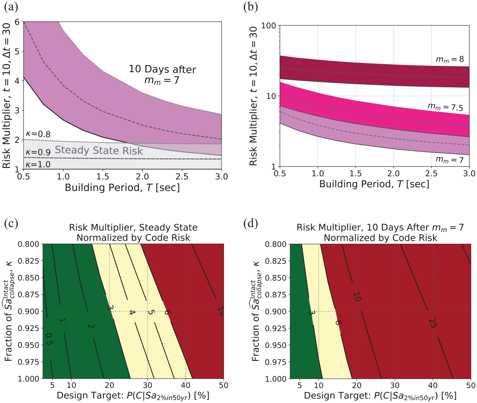
First, consider the effect of building damage (without the elevated aftershock hazard) on the RMs. The gray band in Figure 11a shows the steady-state RMs for code-compliant (i.e. $P (C | S a_{2 % in 50 yr}) = 10 %$ ) buildings with a range of periods, $T$ , and varying levels of earthquake-induced damage, $κ$ . The lower edge of the band corresponds to $RMs = 1$ because $κ = 1$ (the building is intact), and the ground motion hazard is back to the premainshock steady state. Building damage corresponding to $κ = 0.9 and 0.8$ results in increased risk, as indicated by the dashed and dotted lines at ~ $1.5$ and ~ $2$ , respectively. The band is roughly horizontal, indicating minimal variability in the steady-state risk across building periods.

Figure 11.

Risk multipliers, for buildings with a range of periods, design target criteria, and mainshock damage: (a) Risk due to the steady-state hazard (transparent gray) or the elevated hazard 10 days after a $m_{m} = 7$ mainshock (purple). Each band is marked by solid, dashed, and dotted lines for increasing levels of damage ( $κ$ : Fraction of ${\hat{Sa}}_{collapse}^{Intact} = 1.0, 0.9, 0.8$ , respectively). The building design target is the assumed code risk, $P (C | S a_{2 % in 50 yr}) = 10 %$ ; therefore, $κ = 1.0$ for the steady-state risk equals 1; (b) risk due to the elevated hazard 10 days after each mainshock magnitude; (c) schematic tagging criteria based on RMs for steady-state risk. Colors range between dark green for $\leq 3 x$ code risk and dark red for $\geq 6 x$ code risk (see the text for additional discussion). The building period is held constant $(T = 1.0 s)$ while varying the design targets and building damage, $κ$ ; (d) same tagging criteria, during the elevated hazard 10 days after a $m_{m} = 7$ mainshock.

Next, consider the effect of aftershock hazard, which elevates the hazard curve over the steady-state hazard (dotted versus dashed hazard curves in Figure 10). As shown by the purple band in Figure 11a, for 10 days after a $m_{m} = 7$ mainshock, the RMs increase for all building periods and all levels of damage, rising to a RM of ~ $2.5$ for an intact $T = 1.0$ -s building ~ $1.8$ for an intact $T = 2.3$ -s building. The reason for the higher risk at short periods is discussed in the supplemental document.

The RMs associated with the $m_{m} = 7$ mainshock are on the same order of magnitude as the steady-state risk, owing to the moderate increase in aftershock hazard following the $m_{m} = 7$ mainshock. However, as shown in Figure 11b, the elevated risk following a $m_{m} = 8$ mainshock is up to an order of magnitude higher than the risk following a $m_{m} = 7$ , particularly for $T \geq 2$ s. The plots in Figure 11b further show that the elevated hazard’s risk contribution tends to dominate the risk contribution due to damage (the amplitude versus the width of each band), especially for high-magnitude mainshocks.

The building reoccupancy evaluation (i.e. tagging) criteria can be evaluated based on the damage level, $κ$ , with respect to the building code design target of the intact building. This reasoning follows Bazzurro et al. (2004)’s conceptual tagging criteria that allow more damage in buildings that are designed with higher collapse capacity, that is, those with a lower steady-state risk. The contour lines in Figure 11c link buildings with equivalent steady-state risk. For example, an intact $(κ = 1)$ building with a risk equal to the building code target $(P (C | S a_{2 % 5 in 50 yr}) = 10 %)$ has the same risk $(RM = 1)$ as a building that began with an intact collapse risk target of $P (C | S a_{2 % 5 in 50 yr}) = 5 %$ , yet has sustained $κ = 0.8$ worth of damage. Alternatively, an intact building with an initial higher collapse risk (e.g. $P (C | S a_{2 % in 50 yr}) = 25 %$ ) has the same risk $(RM = 3)$ as a building that began with an intact collapse risk target of $P (C | S a_{2 % 5 in 50 yr}) ~ 15 %$ , yet has sustained $κ = 0.8$ worth of damage. Note that for the intact buildings (on the horizontal axis of Figure 11c), the RM is related but not equal to the change in $P (C | S a_{2 % 5 in 50 yr})$ . For example, for the intact building with a RM of 3, the ratio of $P (C | S a_{2 % 5 in 50 yr})$ to the design target is 25/10 = 2.5.

The green, yellow, and red fill colors in Figure 11c correspond to the Yeo and Cornell (2004) RM tagging thresholds for commercial and office buildings: $3 and 6 \times λ_{collapse}^{CodeRisk}$ . Buildings to the lower-left of the contour line for $RMs = 3$ are considered accessible, that is, have a green tag. Conversely, building to the upper-right of the contour line for $RMs = 6$ is considered unsafe to occupy, that is, have a red tag. Yeo and Cornell (2004) suggest that buildings in the light yellow area between these lines should be accessible to individuals who are aware of and accept the increased risk. Based on a strict interpretation of these thresholds, any buildings with an initial $P (C | S a_{2 % 5 in 50 yr}) > 40 %$ should be red-tagged even before a mainshock, due to their steady-state risk in the undamaged state. While the interpretation of results for seismically deficient existing buildings goes beyond the focus of postearthquake assessments, the issue highlights similar complexities for postearthquake decisions regarding reoccupancy.

The results in Figure 11d are similar to those of Figure 11c, but consider the elevated hazard 10 days after a $m_{m} = 7$ mainshock. Due to the elevated hazard, the contour line between $P (C | S a_{2 % 5 in 50 yr}) = 10 %, κ = 1.0$ and $P (C | S a_{2 % 5 in 50 yr}) = 5 %, κ = 0.8$ increases to $RM = 3$ , compressing the green region of the plot. The yellow region is similarly shifted and compressed. In this case, an intact building with $P (C | S a_{2 % 5 in 50 yr}) = 20 %$ will exceed the red tag threshold of $6 \times λ_{collapse}^{CodeRisk}$ , as would a code-conforming building $(P (C | S a_{2 % 5 in 50 yr}) = 10 %)$ that has sustained $κ = 0.8$ worth of damage. As noted in the case study for the individual building, this methodology could be used to establish the number of days required until the risk decays to acceptable risk targets. If one were to assess the risk following a $m_{m} = 8$ mainshock (not shown), the entire matrix of buildings would fall into the red tag region; even the risk for the intact code representative building increases to almost $20 \times λ_{collapse}^{Code Risk}$ . Based on the $\geq 6 x λ_{collapse}^{Code Risk}$ criterion, the entire inventory would be inaccessible 10 days after a $m_{m} = 8$ . As with Figure 11c red tags for seismically deficient existing buildings, such a tagging criterion may not be feasible in the complexity of broader postearthquake considerations.

Rather than using red tags to restrict occupancy immediately following a high-magnitude mainshock, the intact building design targets (x-axis) could be used to inform postmainshock mandatory retrofits. For example, after the Kaikōura earthquake in 2016, New Zealand implemented a mandatory retrofit program for unreinforced masonry (URM) buildings as part of the Earthquake Prone Building policy (Tong et al., 2022). This policy was informed by life-safety risk studies that identified URM buildings as particularly vulnerable and evaluated the life-safety improvement due to various levels of retrofit requirements.

Regardless of the tagging criteria or retrofit policies employed, this elevated risk methodology offers a powerful way to quantify and communicate building collapse risks to inform postearthquake decisions.

Discussion of hazard model assumptions

“The Elevated Hazard Model” section describes the Yeo and Cornell (2009) APSHA model and shows how it can be combined with conventional PSHA to define an elevated postearthquake hazard, which dissipates back to a steady state over time. The collapse risk studies for an individual building and a parametric study demonstrate how the elevated hazard, combined with reductions in building collapse capacity due to earthquake damage, can be used for postearthquake assessment of building safety. The analyses demonstrate that the elevated aftershock hazard is a significant contributor to collapse risk, particularly for mainshock earthquakes with $m_{m}$ greater than 7.

The terms in the APSHA model (Equation 3) provide a framework for linking aftershock rates with the probability of exceeding shaking intensities, given the occurrence of an aftershock. As such, neither the assumptions in this case study nor those in the original case study (Yeo and Cornell, 2009) should be seen as constraints on how the model can be used. To facilitate further exploration of these topics, a few of the assumptions in this case study are discussed here. The discussion is concluded with Figure 12, showing the results from a forward propagation of uncertainty for parameters relating to ruptures following the mainshock event. More details on the sensitivity analyses are included in the supplemental document.

Figure 12.

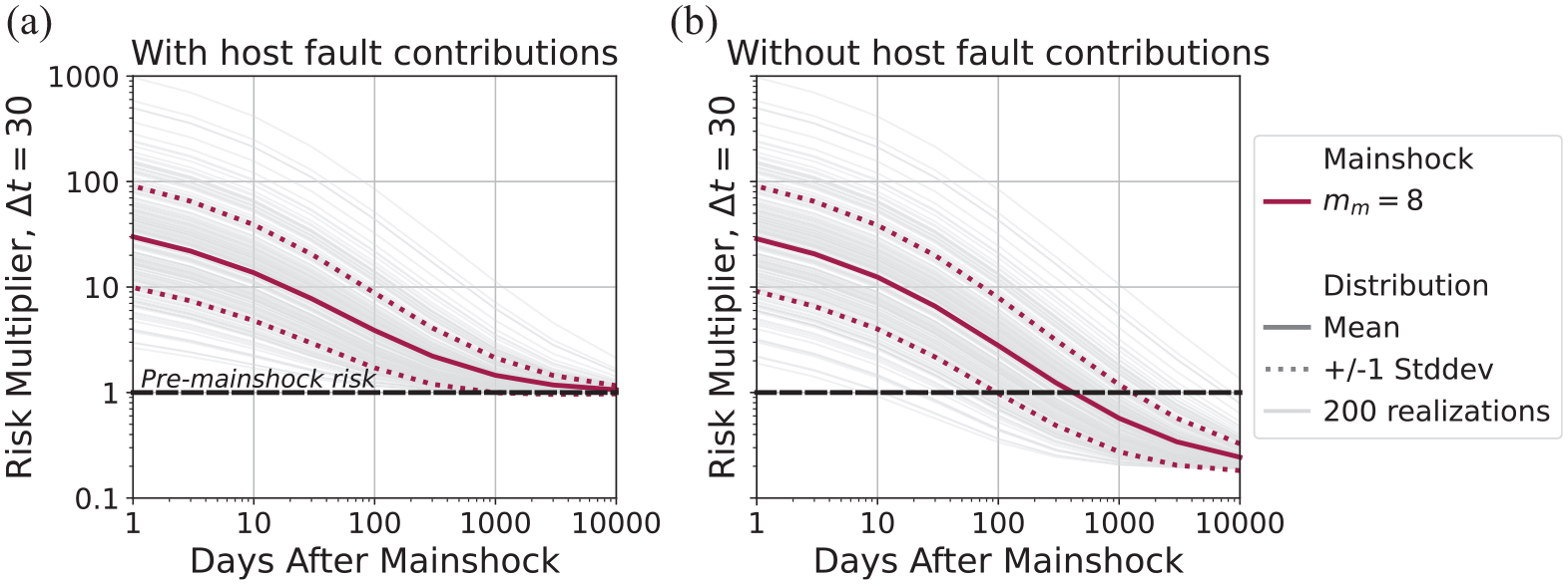
Forward propagation of uncertainty for the elevated collapse risk following a $m_{m} = 8.0$ mainshock. The steady-state hazard in (a) includes contributions from the mainshock host fault, while (b) suppresses future mainshock contributions from the host fault.

Ground motion model (GMM)

GMMs rely on recorded ground motion records to characterize the range of shaking intensities that could result from an earthquake rupture event. The difference between ground motion intensities of the mainshock and aftershock events is an important yet unresolved question. The Boore et al. (2014) GMM (BSSA14, used in the case study) does not differentiate between the two types of events. The case study results suggest that the risk due to elevated hazard decreases for buildings with longer periods (Figure 11b). In contrast, the Chiou and Youngs (2008) (CY08) GMM includes an adjustment for aftershocks, whereby the long period portion of the spectrum is higher for aftershocks than for mainshocks. A reassessment of the results using the CY08 GMM aftershock adjustment suggests the risk increases with building period (i.e. for taller buildings), rather than decreasing as in the case study. Such an effect would be particularly relevant for evaluating postearthquake recovery of dense downtown regions of cities, including considerations related safety cordons (e.g. Hulsey et al., 2022), where cordons around a damaged tall building would restrict access to more neighboring buildings than cordons around shorter buildings.

The BSSA14 GMM is also not dependent on the depth to the top of the rupture, $Z_{tor}$ . This makes the case study insensitive to the assumption of whether the aftershock rupture reaches the surface. In contrast, the CY08 GMM is dependent on $Z_{tor}$ , which would necessitate making an assumption as to whether aftershocks rupture to the surface.

Many well-known GMMs have been updated to include new ground motion records as part of the Next Generation Attenuation (NGA) West2 project (Ancheta et al., 2013). While the CY08 and Abrahamson et al. (2014) GMMs include an aftershock flag that increases the aftershock intensities at longer periods, the updated Chiou and Youngs (2014) GMM no longer includes an aftershock flag. As already noted, the Boore et al. (2014) GMM used in the case study found practically no difference in the between-event residuals for aftershocks versus mainshocks and, therefore, estimates the same amplitudes for both event types.

The limited data for large-magnitude aftershock events present a significant challenge to reliably assessing the aftershock hazard and risk. For example, the ratio between the CY08 GMM aftershock and mainshock intensities varies by period but not by magnitude or distance. As more structural engineering studies consider risk due to aftershock events, it is crucial to better understand the nature of aftershock ruptures and the ground motions they produce. As suggested during the initial discussion of GMMs, a study for use in decision-making would ideally consider the epistemic uncertainty in GMMs via logic trees.

Aftershock event distribution

The event distribution assumptions control the aftershock magnitudes and locations. Yeo and Cornell (2009) used the bounded Gutenberg–Richter recurrence law, limiting the shaking intensity that can be generated by capping the aftershock magnitudes at the mainshock magnitude, $m_{u} = m_{m}$ . Bath’s law (Båth, 1965) suggests that the maximum aftershock magnitude is typically one unit smaller than the mainshock magnitude (e.g. $M_{w} 7$ following a $M_{w} 8$ ). However, there is a non-negligible probability that an aftershock will be larger than the mainshock, as calculated in the work by Reasenberg and Jones (1989). Therefore, this upper bound should be selected carefully, perhaps including a sensitivity study to determine how the maximum aftershock magnitude assumption affects the elevated collapse risk. The case study assumptions on the aftershock rupture length and its location within the mainshock rupture constrain the possible magnitudes to $m_{u} \leq m_{m}$ . As such, aftershock magnitudes that are larger than the mainshock are not considered in this study, but they could be considered using other assumptions for the distribution of rupture locations.

The case study used the Wells and Coppersmith (1994) relationship for the surface rupture length of the aftershock ruptures, given their magnitude, but it did not consider uncertainty in the coefficients of this relationship. The variability for the magnitude to surface rupture length relationship is lognormally distributed for strike-slip faults (per Wells and Coppersmith, 1994). This parameter was included in the forward propagation of uncertainty for Figure 12, using inverse transform sampling from the lognormal cumulative distribution function.

The Yeo and Cornell (2009) location distribution assumes that the aftershocks occur on the same fault, within the same rupture surface as the mainshock. Yet, just as the steady-state hazard can be modeled as either known faults or area sources, aftershock location models can also take various forms. San Francisco’s earthquake hazard is driven by well-mapped faults, so it is reasonable to model the aftershocks on the same faults. However, this assumption may not be appropriate for other tectonic regions such as Christchurch, New Zealand, or Italy. For example, Italy’s steady-state hazard is characterized by area sources. Iervolino et al. (2020) carried this assumption into the APSHA by using an area distribution centered on the mainshock’s hypocenter (Utsu, 1969). Boyd (2012) discussed the merits of both these models. Han et al. (2015) went even further in developing an event distribution that is representative of the cluster-specific aftershock hazard, drawing on other work that carefully considered not only the maximum magnitudes and the location but also the aftershock ground motions as compared with those of the mainshock (Lee and Foutch, 2004; Li and Ellingwood, 2007; Sunasaka and Kiremidjian, 1993). Or, as discussed in the next section, the event distribution could be linked to the aftershock rate by using a spatiotemporal model, such as the epidemic type aftershock sequence (ETAS) model or the hybrid short-term earthquake probabilities (STEP) and Coulomb model.

Rate of aftershock occurrence

The final term in the APSHA methodology characterizes the rate of aftershock occurrences in time. The generic aftershock parameters include uncertainty on the base rate, $a$ (Hardebeck et al., 2019), which was not considered in the case study. Therefore, the variability in $a$ was also included in the forward propagation for Figure 12, using inverse transform sampling from a normal distribution.

Furthermore, while the case study considers the postearthquake environment for possible future scenario earthquakes, the framework would also be relevant in the aftermath of a real event. In such a case, Bayesian updating could be used for the parameters, as suggested by Page et al. (2016), which would reduce the need for the forward propagation of uncertainty.

The case study followed Yeo and Cornell (2009) in using the Reasenberg and Jones (1989) model for aftershock rate of occurrence. By choosing a temporal-only model, the rate of occurrence is independent of aftershock event distributions for magnitude and location. This independence makes the APSHA very flexible, allowing the modules to be refined independently of each other. However, spatiotemporal models could also be incorporated, albeit with more complicated bookkeeping. Like Reasenberg and Jones (1989), epidemic-type aftershock sequence models (ETAS, e.g. Ogata and Zhuang, 2006) and the short-term earthquake probability model (STEP, Gerstenberger et al., 2005) are derived from the statistically based modified Omori’s law and the Gutenberg–Richter recurrence law. Alternatively, the physics-based Coulomb stress method or the Steacy et al.’s (2013) hybrid model could be used to more directly consider how earthquake ruptures affect the surrounding region through changes in static stress (e.g. Dieterich, 1994). The APSHA methodology could be adjusted to incorporate any of these aftershock rate models.

Steady-state hazard

Finally, the assumptions for the steady-state hazard were considered. The case study maintained the same steady-state hazard before and after the mainshock event. This is consistent with the Poissonian assumption that the average time interval between (nonaftershock) events is constant, though the intervals between each event are random and independent. This assumption has been statistically demonstrated and is common in seismic hazard analysis. However, the assumption is in conflict with the elastic rebound theory (Reid, 1908), which suggests that a rupture releases the built-up elastic strain energy, reducing the likelihood that it will rupture again in the near future. To evaluate the relative impact of this theory, the San Andreas fault was removed from the event catalog before recalculating the steady-state hazard. This eliminated the potential for future mainshock events from the fault on which the mainshock originated (the host fault). The elevated collapse risk with and without the host fault contributions is shown in Figure 12a and b, respectively. As expected, removing the host fault causes the elevated collapse risk to decay to a RM lower than 1, since the steady-state risk is lower after the mainshock than before the mainshock. On the contrary, the difference in risk is comparatively less within 100 days of the mainshock. While this approach demonstrates the extreme of suppressing any future mainshock events on the host fault, it also introduces many other assumptions, including how much of the fault should be suppressed and how its contribution would be reintroduced. The use of the elastic rebound theory versus the Poissonian assumption is an ongoing debate among the seismological and earthquake engineering research communities. For example, the Kaikōura, New Zealand earthquake in 2016 is considered an unusual anelastic rupture, challenging the assumption regarding elastic strain release (Diederichs et al., 2019).

The study for the forward propagation of uncertainty included 200 realizations of the elevated collapse risk for the 20-story building after a $m_{m} = 8$ mainshock, assuming that it sustained no structural damage during the mainshock. As noted previously, the steady-state risk in Figure 12a includes the host fault contributions while Figure 12b does not. While the mean elevated collapse risk (solid line) with the host fault contributions is roughly equivalent to the $m_{m} = 8$ risk in Figure 9a, there is large uncertainty around this central estimate. For instance, immediately after mainshock, the RM distribution ranges from 10 to 100 for ±1 standard deviation from the mean. Using the same tagging criterion as before $(RM \geq 6)$ , the time until reoccupancy ranges from 5 to 200 days after the mainshock. This level of uncertainty motivates further studies to reduce the variability in the aftershock occurrence rate and the magnitude to rupture length relationship. This is particularly relevant in the context of operational earthquake forecasting (Jordan et al., 2014). The proposed framework could expand the conversation on operational earthquake forecasting from hazard alone to the risk of building collapse, including the effect of damage sustained during the mainshock. Regardless of the application, the results presented here offer insight into the questions posed at the beginning of the case study.

In summary, the most appropriate choices for the GMM, the event distribution model, the aftershock rate model, and the steady-state hazard assumptions would depend on the specific objectives of the study, as well as knowledge of the local earthquake sources. An informed researcher can incorporate any number of refinements as they implement the elevated hazard model for their own use.

Discussion of damaged building collapse fragility assumptions

The effect of structural damage on the collapse fragility is captured by the trilinear relationship between a relevant DI and the shift in the median value of the fragility function $(κ)$ , as proposed by Galvis et al. (2023). This relationship is the product of a simulation approach that involves a large number of IDAs using back-to-back NLRHAs for the building of interest.

Selecting the relevant DI for this purpose should follow the methodology proposed by Galvis et al. (2023), in which an appropriate DI has four characteristics: (1) be efficient in predicting the collapse safety of damaged buildings, (2) be observable or easily estimated, (3) have a relationship that is relatively insensitive to building height, and (4) be relatively insensitive to modeling uncertainty.

The Galvis et al. (2023) methodology has five steps for selecting a DI from a set of candidates. The candidate set is identified by engineering judgment, in consideration of the raw data from back-to-back IDAs. The first step fits a trilinear relationship to predict $κ$ as a function of each candidate DI. The second step uses the fitting error of the trilinear models to measure the prediction efficiency of each DI. The DIs with the highest fitting errors should be discarded. The third step identifies the optimal threshold for each DI, based on a metric of accuracy in categorizing whether the structure’s performance has reduced beyond a given limit for median collapse capacity. The fourth step uses a sensitivity approach to assess the robustness of the safety thresholds with respect to model uncertainty. The DIs with thresholds that change significantly due to modeling uncertainty should be discarded. The fifth step uses the remaining DIs and their optimal thresholds to recommend quantitative safety criteria for a particular structural type. The collapse fragilities for damaged structures can be computed as an optional sixth step, conditioned on the selected damaged indicator using the fitted trilinear relationship.

For ductile RC moment frames, the peak story drift ratio complies with the first two characteristics desired in the DI (efficiency and ease of estimation/measurement). However, it is outperformed by other DIs—such as the fraction of damaged components—in terms of their robustness to the number of stories and modeling uncertainty. Applications of this framework should further explore the implications of selecting other DIs on which to condition damaged collapse fragilities for each structural system of interest.

Summary and conclusion

This article provides a framework to (1) identify the mainshock magnitudes that pose a relevant aftershock concern for a location of interest and (2) quantify how long it takes for the aftershock hazard to dissipate. A sensitivity study is also included to (3) highlight the most important gaps in current knowledge that deserve further attention and research from the earthquake engineering and seismology communities.

The proposed framework extends the APSHA model (Yeo and Cornell, 2009) by combining the aftershock and steady-state hazards to obtain an elevated postearthquake hazard curve. Yeo and Cornell (2009) assume that the aftershock occurs on the same fault and rupture surface as the mainshock, which is assumed to be appropriate for tectonic settings such as the vertical strike-slip faults in the San Francisco Bay Area. The elevated hazard allows the framework to quantify building collapse risk following a mainshock at different points in time, considering the relative contributions of aftershock activity and the destabilizing effects of building damage sustained during the mainshock.

This article demonstrates the proposed framework with a case study for a 20-story RC frame building located in downtown San Francisco. The mainshocks are assumed to rupture the portion of the fault closest to the city as worst-case scenarios. Based on the case study and the associated modeling assumptions, the elevated collapse risk for buildings in downtown San Francisco is highly dependent on the magnitude of the mainshock event on the San Andreas Fault. For a $m_{m} = 7$ , the elevated hazard causes a relatively small increase in risk (a RM of approximately 2 compared with premainshock conditions) that dissipates back to the steady-state risk in about 3 months. Thus, structural damage is more relevant than the elevated hazard for mainshocks of $m_{m} \leq 7$ . In contrast, the aftershock hazard following a $m_{m} = 8$ mainshock would increase the building collapse risk above that of the steady-state hazard for 3 years, with a larger impact than building damage. That said, the collapse capacity drops off steeply for damage greater than the DI threshold, such that Galvis et al. (2023) recommend red-tagging regardless of the mainshock magnitude. For mainshock events greater than $m_{m} = 7$ , the postearthquake risk of building collapse is controlled by a combination of the elevated aftershock hazard, which dissipates over time following the mainshock, and the amount of structural damage the building has incurred. In such cases, the proposed framework would be effective for evaluating building safety levels (i.e. an acceptable RM) to inform decisions regarding building recoccupancy and cordoning following the earthquake. For instance, the RM of the case study building after the $m_{m} = 8$ remains above 1 (the steady-state value) for over 3 years. However, decision-makers could allow reoccupancy for $RM < 6$ , in which case a building without apparent damage could be reoccupied approximately 40 days after the mainshock. Alternatively, they could assess the RMs for an inventory of buildings (as done in the parametric study) to define a tagging criterion/retrofit policy that balances the elevated collapse risk against the societal risks associated with mass building closures. Such decisions have important implications for postearthquake functional recovery and community resilience.

The results of the case study are subject to modeling assumptions, which were discussed to shed light on potential areas of future research (see the supplemental document for more details). The sensitivity study demonstrated that the most important assumptions in the framework (aside from the San Francisco region-specific assumptions regarding geology) are the selection of the GMM, the uncertainty in the base aftershock rate, the magnitude to rupture length relationship, and the inclusion or removal of the host fault when calculating the steady-state contribution of the elevated hazard. Therefore, these parameters were included in a forward propagation of uncertainty. These case studies demonstrate the useful insights that are provided by the elevated collapse risk framework for risk-based decision-making to facilitate postearthquake recovery.

Supplemental Material

sj-pdf-1-eqs-10.1177_87552930231220549 – Supplemental material for Elevated collapse risk based on decaying aftershock hazard and damaged building fragilities

Supplemental material, sj-pdf-1-eqs-10.1177_87552930231220549 for Elevated collapse risk based on decaying aftershock hazard and damaged building fragilities by Anne M Hulsey, Francisco A Galvis, Jack W Baker and Gregory G Deierlein in Earthquake Spectra

Footnotes

Acknowledgements

The first author would like to thank Dr Ganyu Teng for a brief discussion that led to the idea of combining the steady-state and aftershock hazards into one “elevated” hazard. Two anonymous reviewers challenged the authors to test the sensitivity to the aftershock model assumptions, which prompted the sensitivity studies that are presented in the supplemental document and resulted in a stronger and more nuanced study.

Declaration of conflicting interests

The author(s) declared no potential conflicts of interest with respect to the research, authorship, and/or publication of this article.

Funding

The author(s) received no financial support for the research, authorship, and/or publication of this article. This project was funded by Stanford University, and a FEMA graduate fellowship (awarded through the Earthquake Engineering Research Institute).

ORCID iDs

Anne M Hulsey

Francisco A Galvis

Jack W Baker

Data and resources

A supplemental document is included with this publication. The following items can be found at: Hulsey, A., Galvis, F., Baker, J. W., Deierlein G. G. (2023) “Analysis scripts and data to reproduce paper figures,” in Elevated Collapse Risk Based on Decaying Aftershock Hazard and Damaged Building Fragilities. DesignSafe-CI.

Inputs for the case study including:

an event catalogue for steady-state hazard,

parameters for the aftershock environment,

and damaged building fragility data for the 4-, 8-, 12-, and 20-story buildings.

Jupyter notebooks written in python for

calculating the elevated hazard,

calculating the steady-state hazard,

conducting the individual building case study,

conducting a forward propagation of uncertainty,

and conducting the parametric risk study.

Supplemental material

Supplemental material for this article is available online.

References

Aagaard

Blair

Boatwright

Garcia

Harris

Micheal

Schwartz

DiLeo

(2016) Earthquake outlook for the San Francisco Bay Region 2014–2043 (version 1.1, August 2016). Technical report, U.S. Geological Survey Fact Sheet 2016-3020, June.

Abrahamson

Silva

Kamai

(2014) Summary of the ASK14 ground motion relation for active crustal regions. Earthquake Spectra 30(3): 1025–1055.

ACI 318-05 (2005) Building Code Requirements for Structural Concrete (ACI 318-05). Farmington Hills, MI: American Concrete Institute.

Altoontash

(2004) Simulation and damage models for performance assessment of reinforced concrete beam-column joints. Technical report, Stanford University, Stanford, CA, February.

Ancheta

Darragh

Stewart

Seyhan

Silva

Chiou

BSJ

Wooddell

Graves

Kottke

Boore

Kishida

Donahue

(2013) PEER NGA-West2 database, technical report PEER 2013/03. Technical report, Peer Earthquake Engineering Research Center, Berkeley, CA, May 2.

ASCE 7-02 (2002) Minimum design loads and associated criteria for buildings and other structures: ASCE/SEI 7-02. Technical report, American Society of Civil Engineers, Reston, VA.

ATC-20-1 (2015) Field manual: Postearthquake safety evaluations of buildings (2nd Edition). Technical report, Applied Technology Council, Redwood City, CA

Baker

(2015) Efficient analytical fragility function fitting using dynamic structural analysis. Earthquake Spectra 31(1): 579–599.

Baker

Jayaram

(2008) Correlation of spectral acceleration values from NGA ground motion models. Earthquake Spectra 24(1): 299–317.

10.

Båth

(1965) Lateral inhomogeneities of the upper mantle. Tectonophysics 2(6): 483–514.

11.

Bazzurro

Cornell

Menun

Motahari

(2004) Guidelines for seismic assessment of damaged buildings. In: 13th World Conference on Earthquake Engineering, Vancouver, BC, Canada, 1–6 August.

12.

Boore

Stewart

Seyhan

Atkinson

(2014) NGA-West2 equations for predicting PGA, PGV, and 5% damped PSA for shallow crustal earthquakes. Earthquake Spectra 30(3): 1057–1085.

13.

Boyd

(2012) Including foreshocks and aftershocks in time-independent probabilistic seismic-hazard analyses. Bulletin of the Seismological Society of America 102(3): 909–917.

14.

Burton

Deierlein

(2018) Integrating visual damage simulation, virtual inspection, and collapse capacity to evaluate post-earthquake structural safety of buildings. Earthquake Engineering & Structural Dynamics 47(2): 294–310.

15.

Chiou

BSJ

Youngs

(2008) An NGA model for the average horizontal component of peak ground motion and response spectra. Earthquake Spectra 24(1): 173–215.

16.

Chiou

BSJ

Youngs

(2014) Update of the Chiou and Youngs NGA model for the average horizontal component of peak ground motion and response spectra. Earthquake Spectra 30(3): 1117–1153.

17.

Cordova

Deierlein

Mehanny

Cornell

(September 2000) Development of a two-parameter seismic intensity measure and probabilistic assessment procedure. In: The Second US-Japan Workshop on performance-based earthquake engineering methodology for reinforced concrete building structures, Sapporo, Hokkaido, pp. 187–206.

18.

Cornell

(1968) Engineering seismic risk analysis. Bulletin of the Seismological Society of America 58(5): 1583–1606.

19.

Cornell

Vanmarcke

(January 1969) The major influences on seismic risk. In: The 4th world conference on earthquake engineering, Santiago, Chile.

20.

Davalos

(2018) Improved Methodologies for Seismic Collapse Risk Estimation. PhD Thesis, Stanford University, Stanford, CA.

21.

Diederichs

Nissen

Lajoie

Langridge

Malireddi

Clark

Hamling

Tagliasacchi

(2019) Unusual kinematics of the Papatea fault (2016 Kaikōura earthquake) suggest anelastic rupture. Science Advances 5(10): eaax5703.

22.

Dieterich

(1994) A constitutive law for rate of earthquake production and its application to earthquake clustering. Journal of Geophysical Research 99(B2): 2601–2618.

23.

Eads

Miranda

Lignos

(2015) Average spectral acceleration as an intensity measure for collapse risk assessment. Earthquake Engineering & Structural Dynamics 44(12): 2057–2073.

24.

FEMA (2009) Quantification of building seismic performance factors. Technical report, Applied Technology Council, Redwood City, CA, April.

25.

Field

Dawson

Felzer

Frankel

Gupta

Jordan

Parsons

Petersen

Stein

Weldon

Wills

(2008) The uniform California earthquake rupture forecast, Version 2 (UCERF 2), USGS Open file report 2007-1437. Technical report, US Geological Survey, Reston, VA.

26.

Galvis

Hulsey

Baker

Deierlein

(2023) Simulation-based methodology to identify damage indicators and safety thresholds for post-earthquake evaluation of structures. Earthquake Engineering & Structural Dynamics 3: 1–22.

27.

Gardner

Knopoff

(1974) Is the sequence of earthquake in Southern California, with aftershocks removed, Poissonian? Bulletin of the Seismological Society of America 64(5): 1363–1367.

28.

Gerstenberger

Wiemer

Jones

Reasenberg

(2005) Real-time forecasts of tomorrow’s earthquakes in California. Nature 435(7040): 328–331.

29.

Goda

Taylor

(2012) Effects of aftershocks on peak ductility demand due to strong ground motion records from shallow crustal earthquakes. Earthquake Engineering & Structural Dynamics 41: 2311–2330.

30.

Gomberg

Ludwig

Bekins

Brocher

Brock

Brothers

Chaytor

Frankel

Geist

Haney

Hickman

Leith

Roeloffs

Schulz

Sisson Thomas

Wallace

Watt

Wein

(2017) Reducing risk where tectonic plates collide — U.S. Geological survey subduction zone science plan. Technical report, U.S. Geological Survey Circular 1428, Reston, VA, June17.

31.

Gutenberg

Richter

(1944) Frequency of earthquakes in California. Bulletin of the Seismological Society of America 34(4): 185–188.

32.

Han

Van De Lindt

(2015) Assessment of seismic performance of buildings with incorporation of aftershocks. Journal of Performance of Constructed Facilities 29(3): 1–17.

33.

Hardebeck

Llenos

Michael

Page

van der Elst

(2019) Updated California aftershock parameters. Seismological Research Letters 90(1): 262–270.

34.

Haselton

Liel

Lange

(2008) Beam-column element model calibrated for predicting flexural response leading to global collapse of RC frame buildings, PEER report 2007 03, Pacific Earthquake Engineering Research Center, University of California, Berkeley, CA, May.

35.

Hulsey

Baker

Deierlein

(2022) High-resolution post-earthquake recovery simulation: Impact of safety cordons. Earthquake Spectra 38(3): 2061–2087.

36.

Ibarra

Medina

Krawinkler

(2005) Hysteretic models that incorporate strength and stiffness deterioration. Earthquake Engineering and Structural Dynamics 34(12): 1489–1511.

37.

Iervolino

Chioccarelli

Suzuki

(2020) Seismic damage accumulation in multiple mainshock-aftershock sequences. Earthquake Engineering and Structural Dynamics 49: 1007–1027.

38.

Jalayer

Ebrahimian

(2017) Seismic risk assessment considering cumulative damage due to aftershocks. Earthquake and Structures 46: 369–389.

39.

Jayaram

Lin

Baker

(2011) A computationally efficient ground-motion selection algorithm for matching a target response spectrum mean and variance. Earthquake Spectra 27(3): 797–815.

40.

Jordan

Marzocchi

Michael

Gerstenberger

(2014) Operational earthquake forecasting can enhance earthquake preparedness. Seismological Research Letters 85(5): 955–959.

41.

Kohrangi

Bazzurro

Vamvatsikos

(2016) Vector and scalar IMs in structural response estimation, Part I: Hazard analysis. Earthquake Spectra 32(3): 1507–1524.

42.

Krawinkler

Zareian

Medina

Ibarra

(2006) Decision support for conceptual performance-based design. Earthquake Engineering and Structural Dynamics 35(1): 115–133.

43.

Lee

Foutch

(2004) Performance evaluation of damaged steel frame buildings subjected to seismic loads. Journal of Structural Engineering 130(4): 588–599.

44.

Ellingwood

(2007) Performance evaluation and damage assessment of steel frame buildings under main shock–aftershock earthquake sequences. Earthquake Engineering & Structural Dynamics 36(3): 405–427.

45.

Lin

Haselton

Baker

(2013) Conditional spectrum-based ground motion selection. Part I: Hazard consistency for risk-based assessments. Earthquake Engineering & Structural Dynamics 42(12): 1847–1865.

46.

Luco

Bachman

Crouse

Harris

Hooper

Kircher

Caldwell

Rukstales

(2015) Updates to building-code maps for the 2015 NEHRP recommended seismic provisions. Earthquake Spectra 31: S245–S271.

47.

Luco

Bazzurro

Cornell

(2004) Dynamic versus static computation of the residual capacity of a mainshock-damaged building to withstand an aftershock. In: 13th World Conference on Earthquake Engineering, Vancouver, BC, Canada, 1–6 August.

48.

Luco

Ellingwood

Hamburger

Hooper

Kimball

Kircher

(September 2007) Risk-targeted versus current seismic design maps for the conterminous United States. In: Structural Engineering Association of California 2007 Convention Proceedings, Squaw Creek, CA, pp. 1–13.

49.

McNamara

Wolin

Moschetti

Thompson

Powers

Shumway

Petersen

Wilson

Benz

(2020) Evaluation of ground-motion models for USGS seismic hazard models using near-source instrumental ground-motion recordings of the Ridgecrest, California, earthquake sequence. Bulletin of the Seismological Society of America 110(4): 1517–1529.

50.

Ogata

Zhuang

(2006) Space-time ETAS models and an improved extension. Tectonophysics 413(1–2): 13–23.

51.

Omori

(1894) On the aftershocks of earthquakes. Journal of the College of Science, Imperial University of Tokyo 7: 111–120.

52.

Page

van Der Elst

Hardebeck

Felzer

Michael

(2016) Three ingredients for improved global aftershock forecasts: Tectonic region, time-dependent catalog incompleteness, and intersequence variability. Bulletin of the Seismological Society of America 106(5): 2290–2301.

53.

Raghunandan

Liel

Luco

(2015) Aftershock collapse vulnerability assessment of reinforced concrete frame structures. Earthquake Engineering & Structural Dynamics 44(3): 419–439.

54.

Reasenberg

Jones

(1989) Earthquake hazard after a mainshock in California. Science 243(4895): 1173–1176.

55.

Reid

(1908) The California earthquake of April 18, 1906: Report of the State Earthquake Investigation Commission, in two volumes and atlas. Technical report, Carnegie Institution, Washington, DC.

56.

Shi

Saygili

Ozbulut

Zhou

(2020) Risk-based mainshock-aftershock performance assessment of SMA braced steel frames. Engineering Structures 212: 110506.

57.

Shokrabadi

Burton

(2018) Risk-based assessment of aftershock and mainshock-aftershock seismic performance of reinforced concrete frames. Structural Safety 73: 64–74.

58.

Shokrabadi

Burton

Stewart

(2018) Impact of sequential ground motion pairing on mainshock-aftershock structural response and collapse performance assessment. Journal of Structural Engineering 144: 04018177.

59.

Steacy

Gerstenberger

Williams

Rhoades

Christophersen

(2013) A new hybrid Coulomb/statistical model for forecasting aftershock rates. Geophysical Journal International 196(2): 918–923.

60.

Sunasaka

Kiremidjian

(July 1993) A method for structural safety evaluation under mainshock-aftershock earthquake sequences. Technical report 105, John A. Blume Earthquake Engineering Center, Stanford, CA.

61.

Tong

Filippova

Ingham

(2022) Effectiveness of unreinforced masonry seismic retrofit programmes: Review of policies in New Zealand and the United States. International Journal of Disaster Risk Reduction 76: 103008.

62.

Toro

Silva

(2001) Scenario earthquakes for Saint Louis, MO, and Memphis, TN, and seismic hazard maps for the Central United States region including the effect of site conditions. Technical report, Prepared under USGS External Grant Number 1434-HQ-97-GR-02981 (Scenario Earthquakes and Seismic Hazard Mapping for the New Madrid Region), January.

63.

Utsu

(1961) A statistical study on the occurrence of aftershocks. The Geophysical Magazine 30: 521–605.

64.

Utsu

(1969) Aftershocks and earthquake statistics (1): Some parameters which characterize an aftershock sequence and their interrelations. Journal of the Faculty of Science, Hokkaido University, Series 7, Geophysics 3(3): 129–195.

65.

Utsu

(1971) Aftershocks and Earthquake Statistics (3): Analysis of the distribution of earthquake in magnitude, time and space with special consideration to clustering characteristics of earthquake occurrence. Journal of the Faculty of Science, Hokkaido University, Series 7, Geophysics 3(5): 379–441.

66.

Utsu

Ogata

(1995) The centenary of the Omori formula for a decay law of aftershock activity. Journal of Physics of the Earth 43(1): 1–33.

67.

Vamvatsikos

Cornell

(2002) Incremental dynamic analysis. Earthquake Engineering & Structural Dynamics 31(3): 491–514.

68.

Vamvatsikos

Cornell

(2004) Applied incremental dynamic analysis. Earthquake Spectra 20(2): 523–553.

69.

Wells

Coppersmith

(1994) New empirical relationships among magnitude, rupture length, rupture width, rupture area, and surface displacement. Bulletin-Seismological Society of America 84(4): 974–1002.

70.

Yeo

Cornell

(2004) Building tagging criteria based on aftershock PSHA. In: 13th world conference on earthquake engineering, Vancouver, BC, Canada, 1–6 August.

71.

Yeo

Cornell

(2009) A probabilistic framework for quantification of aftershock ground-motion hazard in California: Methodology and parametric study. Earthquake Engineering & Structural Dynamics 38(1): 45–60.

72.

Zhang

Burton

Shokrabadi

Wallace

(2019) Seismic risk assessment of a 42-story reinforced concrete dual-system building considering mainshock and aftershock hazard. Journal of Structural Engineering 145(11): 04019135.

Supplementary Material

Please find the following supplemental material available below.

For Open Access articles published under a Creative Commons License, all supplemental material carries the same license as the article it is associated with.

For non-Open Access articles published, all supplemental material carries a non-exclusive license, and permission requests for re-use of supplemental material or any part of supplemental material shall be sent directly to the copyright owner as specified in the copyright notice associated with the article.

0.00 MB

0.72 MB