
Abstract
Although fragility function development for structures is a mature field, it has recently thrived on new algorithms propelled by machine learning (ML) methods along with heightened emphasis on functions tailored for community- to regional-scale application. This article seeks to critically assess the implications of adopting alternative traditional and emerging fragility modeling practices within seismic risk and resilience quantification to guide future analyses that span from the structure to infrastructure network scale. For example, this article probes the similarities and differences in traditional and ML techniques for demand modeling, discusses the shift from one-parameter to multiparameter fragility models, and assesses the variations in fragility outcomes via statistical distance concepts. Moreover, the previously unexplored influence of these practices on a range of performance measures (e.g. conditional probability of damage, risk of losses to individual structures, portfolio risks, and network recovery trajectories) is systematically evaluated via the posed statistical distance metrics. To this end, case studies using bridges and transportation networks are leveraged to systematically test the implications of alternative seismic fragility modeling practices. The results show that, contrary to the classically adopted archetype fragilities, parameterized ML-based models achieve similar results on individual risk metrics compared to structure-specific fragilities, promising to improve portfolio fragility definitions, deliver satisfactory risk and resilience outcomes at different scales, and pinpoint structures whose poor performance extends to the global network resilience estimates. Using flexible fragility models to depict heterogeneous portfolios is expected to support dynamic decisions that may take place at different scales, space, and time, throughout infrastructure systems.
Introduction
Measuring and modeling resilience has become imperative for establishing community resilience baselines, determining actions to improve it, and monitoring its changes (National Academies of Sciences, Engineering, and Medicine, 2019; National Research Council, 2012). A key component of any seismic risk and resilience modeling framework is damage modeling of physical assets, including structures and infrastructure systems (e.g. Cimellaro et al., 2010; Deierlein et al., 2003; van de Lindt et al., 2023). These performance estimates are a precursor for subsequent loss analyses, repair and recovery modeling, and interdependent systems analyses. The common practice is to use fragility functions to predict systems’ performance while recognizing the influence of inherent sources of uncertainty. A fragility function is often defined as the conditional probability of the response of a system exceeding its capacity, expressed as:

where
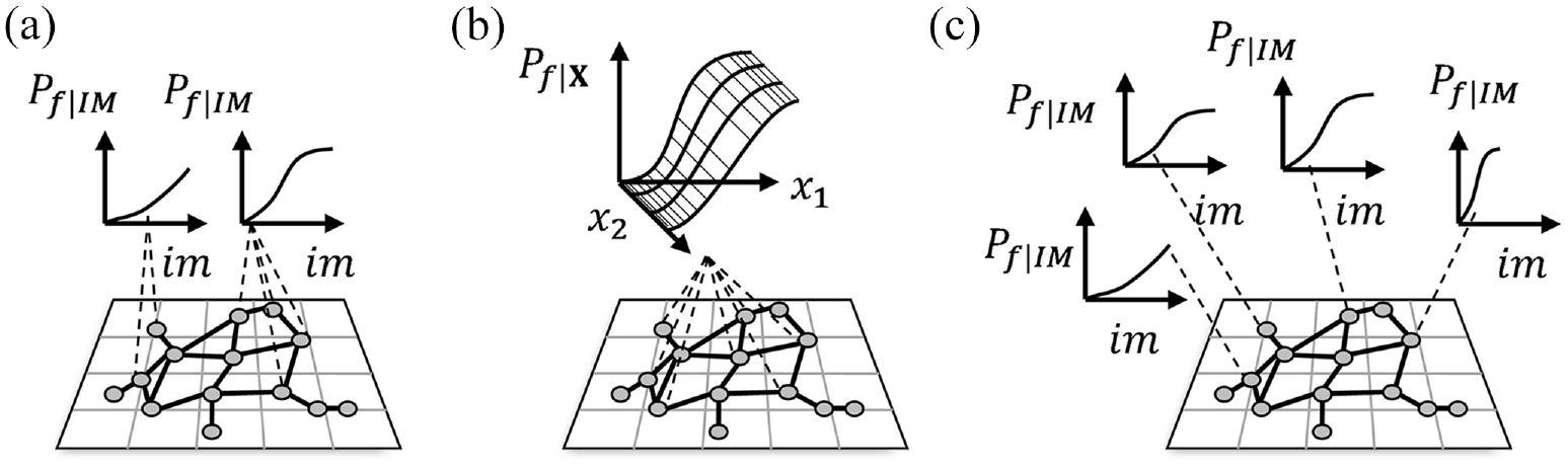
Strategies for assigning fragility functions for regional-scale analysis: (a) archetype fragilities, (b) parameterized fragilities, and (c) structure-specific fragilities.
The limitations of archetype fragilities have propelled a growing body of researchers to propose models that capture variations in the fragility estimate given differences in structural parameters. Modeling each structure separately, as graphically depicted in Figure 1c, may not be feasible; besides, the benefit of such an endeavor is not yet clear. This approach may be hampered by the lack of data to characterize individual structures or by the computational costs associated with nonlinear simulations of thousands of structures across a network. Even if achieved, the derived structure-specific fragilities could become outdated due to aging processes or other situations that can provoke changes in the portfolio (Choe et al., 2008; Ghosh and Padgett, 2011; Rao et al., 2017). Hence, recent studies on analytical fragility derivations have focused on reducing the cost of nonlinear dynamic simulations by either lowering the resolution of the models, utilizing data-driven approaches or a combination of these (e.g. Ghosh et al., 2013; Muntasir Billah and Shahria Alam, 2015; Patsialis and Taflanidis, 2020; Rincon and Padgett, 2022; Seo et al., 2012). The faster computation of the system response, typically achieved through surrogate models, allows more refined analysis at the regional scale. Besides computational efficiency for response prediction, some researchers have exploited such methods to propose more expressive fragility models that capture the portfolio heterogeneity and system conditions. These models assume the failure probability,
This article addresses the unanswered question of how and if different fragility modeling practices (including those that leverage emerging surrogate modeling, machine learning (ML) techniques, and parameterized approaches) actually influence the outcomes of seismic risk and resilience quantification. Along the way we propose a systematic approach for comparing fragility methods that influence a wide range of performance measures that span from the structure to infrastructure network scale. To this end, the next section discusses common steps for the derivation of seismic fragility functions and presents the details of performance measures for comparison of assessment results ranging from the structure level to the network scale (e.g. conditional probability of damage, risk of losses to individual structures, portfolio risks, network recovery trajectories). The theoretical backgrounds, similarities, and differences among fragility modeling approaches are described and applied to case studies that consist of multiple spans simply supported bridges subjected to bidirectional ground motion records. The subsequent section presents the implications of adopting alternative traditional and emerging fragility modeling practices within seismic risk quantification of structures and portfolios, and in the final section, to resilience estimation of infrastructure networks.
Methods
The proposed comparisons are presented in three main steps: (1) derivation and comparison of fragility functions for multiresponse systems, (2) evaluation of implications on risk metrics at the structure and portfolio scale, and (3) measurement of influence on network resilience estimates. This section summarizes the overall steps used for fragility function derivation, while the details of the compared modeling practices are presented in the next section. The following “Methods” subsections present the performance measures proposed in this study to quantify the influence of such practices in risk and resilience outcomes across scales.
Our study evaluates multiresponse systems, that is, structures whose performance (or damage condition) is defined by


Derivation of fragility functions for systems with multiple failure modes
Common fragility derivation techniques share the steps depicted in Figure 2. As shown in the figure, the main difference lies in the procedure used for the estimation of the seismic response (Step 5); hence, we focus our attention on this task. While more details on the investigated techniques are presented in the next section, the general steps are described as follows:
Records selection: a set of representative ground motion records are selected. These are expected to cover a wide range of intensity measures values (e.g. peak ground acceleration). In fact, this suite should be representative of the joint distribution of high-dimensional intensity measure descriptions (i.e. multivariate hazard consistency) (Du and Padgett, 2021). Only unscaled ground motions are used in this study to avoid scale-induced bias (Mai et al., 2017; Sudret et al., 2015).
Model definition and structural variables: the computational model, modeling assumptions and modeling parameters are defined to capture the uncertain and complex system failure modes. For forward uncertainty propagation, modeling parameters that may be significant in the system response may be treated as random variables, represented by the vector
Definition of the experimental design: considering exploration of the entire input space
Nonlinear dynamic analyses: computer algorithms
Construction of demand prediction model and response estimation: the data set
Capacity definition and computation of failure events: the components’ capacities
Fitting a fragility model: while a common approach is to fit lognormal and logistic distributions to the conditional failure probabilities, non-parametric methods can also be used (Lallemant et al., 2015). Multinomial logistic distribution has also been deemed particularly suitable for sequential damage fragility functions (Andriotis and Papakonstantinou, 2018). In this model, the probability of a damage state

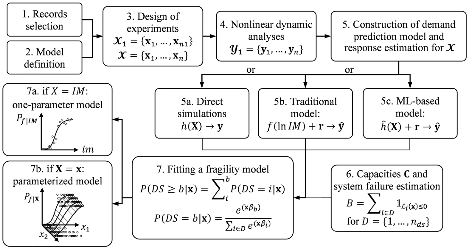
Common steps of fragility derivation practices.
Using multiclass logistic regression, one can obtain the set of coefficients
Implications of fragility derivation methods across risk estimates
Although (visual) comparisons of a “benchmark” fragility model with derived fragilities are commonplace, this strategy offers little information about the expected implications on risk and resilience estimates. Hence, the following subsections explain how we propose to compare the derived fragilities at different scales and across performance measures, considering that outcomes at each stage can be of interest for different stakeholders. The proposed metrics for comparing methods are based on the cumulative distribution function
Statistical comparison between fragility functions
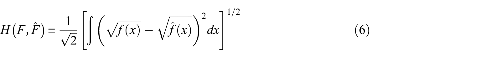
Independent of the type of derivation method, a primary outcome of such fragility analyses is often a single fragility curve that is derived in the form of a univariate function; parameterized fragilities require additional steps to arrive at this form as explained later within the context of the case study. We use statistical concepts to measure the “differences” between the evaluated techniques and a benchmark model. Given that a fragility function resembles a cumulative distribution function (cdf), the Kolmogorov–Smirnov statistic
The


Measurements of differences in structural and regional risk
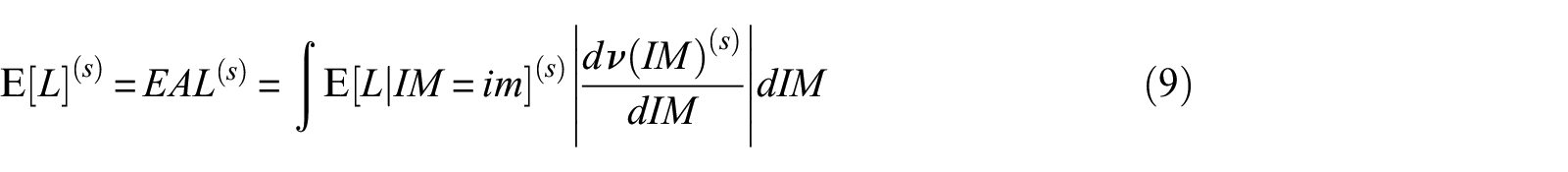
Practical comparisons should be made based on the differences found in reliability, risk, or resilience metrics. These explicitly include the exposure of the assets to site-specific hazards and potential consequences of this exposure (Mahsuli and Haukaas, 2013). As one example, this article considers losses at the structure and portfolio scale when comparing the implication of adopting different fragility methods. Given a defined seismic hazard model, the expected relative loss of a particular structure conditional to the hazard intensity

where
Where
The previous risk metrics can be translated to a portfolio of structures. In this case, other considerations such as spatially correlated hazard intensities (Goda and Hong, 2008; Jayaram and Baker, 2009) must be included, and the analysis may require the use of simulation-based approaches. The computation of relative losses at the structure level is presented in Equation 10, where

To aggregate structural losses across the portfolio, the replacement value

Finally, the expected portfolio annual loss, for a particular fault, is computed as follows:

where
Influence of fragility on network performance measures
An infrastructure system consists of a set of structures connected (or somehow related) to others that work together to serve a system function. In fact, the way system components (i.e. structures in this case) interact with each other may hold more significance when assessing network performance than their individual performance alone, enabling a large body of analyses beyond direct risk metrics (Bocchini and Frangopol, 2011, 2012; Dueñas-Osorio et al., 2007). To evaluate how fragility function derivation practices impacts network functionality, we adopt a select set of performance measures that fall under the general class of time-dependent connectivity-based evaluations. Using a graph
We define network functionality in terms of connectivity-based metrics. For this, we use the concept of network efficiency
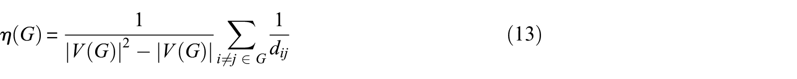
In Equation 13,
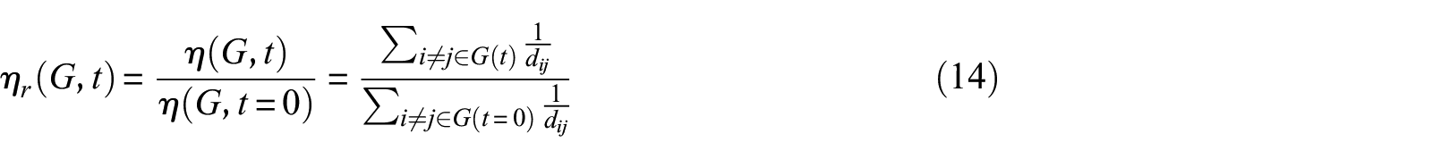
where
Overview of traditional and recent demand prediction models for fragility derivation of multicomponent response systems
This section probes the differences and similarities in traditional and more recent alternative practices for demand modeling (Step 5 in Figure 2). The approaches studied here differ in the way they can relate system and/or hazard features with the multiple system responses, in the extent they propagate input uncertainty into the demand estimation, and in the overall assumptions needed by each one. Each of the methods presented below are further evaluated through illustrative examples in the next sections.
Monte Carlo analysis
Monte Carlo analysis is a straightforward method to propagate uncertainties in the hazard intensity and structure features. A large number of samples
Linear regression model
Foundational work in seismic fragility development often considered the relationship between the intensity measure

where parameters

Besides the linear assumption, the model also assumes a constant variance (homoscedasticity) of the residuals in the log-log scale. Only tens to hundreds of nonlinear analyses are required, which makes it attractive to derive structure-specific fragilities; however, its application to portfolios is hampered by the use of strong assumptions and the need to still perform nonlinear analyses.
Multivariate pdfs at multiple intensity levels
To relax the homoscedastic and linear relationship assumptions, past authors have proposed fitting multivariate pdfs to the logarithm of the responses at discrete intensity values (or bins) (Karamlou and Bocchini, 2015). Although non-parametric versions have been proposed, the multivariate normal distribution is used here given that satisfactory results have been empirically observed. The pdf takes the form
Surrogate-based demand prediction
Using different techniques from the ML field, it is possible to develop more flexible seismic demand models that capture the variability in system configurations (Ghosh et al., 2013; Seo et al., 2012; Xie et al., 2020). ML methods enable more complex structures and are deemed to capture nonlinearities in the functional relationship between

where
Fragility functions derived with different techniques
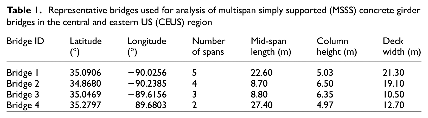
Bridge structures (and their role in transportation network functionality) are adopted to explore the influence of fragility modeling practices, including the demand modeling approach adopted as well as the strategy for mapping fragility model to structure within the portfolio. Non-seismically designed multispan simply supported (MSSS) concrete girder bridges, typical of the central and eastern US (CEUS), are considered to illustrate the systematic comparative assessment across scales and implement the proposed statistical distance measures at distinct stages of analysis. Scripts for three-dimensional nonlinear analytical models, developed in Opensees (McKenna and Feneves, 2023), and a set of 348 unscaled ground motions records (representative of the CEUS region) are retrieved from DesignSafe repositories (Kameshwar et al., 2019). The models retrieved were developed in a parameterized fashion (including geometrical, material, and aging parameters) which facilitates the use of experimental designs for fragility assessment and uncertainty propagation. Slight modifications of these have been performed for the purpose of this study. The different fragility derivation techniques presented above will be illustrated using four different bridge configurations (refer to Table 1). The configurations correspond to existing bridges in the National Bridge Inventory database found in the CEUS region (National Bridge Inventory (NBI), 2022); the locations have been arbitrarily modified in this study.
Representative bridges used for analysis of multispan simply supported (MSSS) concrete girder bridges in the central and eastern US (CEUS) region
Experimental designs
The varying approaches for fragility derivation are contingent on whether the technique aims to generalize to diverse structural configurations or not (i.e. whether the fragility represents a single structure, an entire portfolio or generalizes to any system configuration), which thereby influences the design of experiments employed (Step 3 in Figure 2). Two types of designs of experiments are defined to construct the fragility functions. The first experimental design,
In this study, the traditional methods based on Monte Carlo, multivariate pdfs at multiple intensity levels and linear regression analyses are used to develop structure-specific fragilities for the four case study bridges. The known parameters of these bridges are fixed across samples; the rest of parameters (geometrical, material, and aging parameters) are sampled from probabilistic models defined in previous studies (Ghosh and Padgett, 2011; Kameshwar et al., 2019; Nielson and DesRoches, 2007a). Unrealistic combinations of parameters are avoided by considering design rules and appropriate sampling strategies. A similar strategy is used to create designs representative of the general class of bridges (portfolio fragilities). For this case, the experimental designs include the geometrical parameters shown in Table 1 as random variables. The probabilistic distributions of such parameters are obtained from a statistical analysis of the NBI database and from previous studies (NBI, 2022; Nielson and DesRoches, 2007a). This design is used for building seismic demand models of the archetype and surrogate-based models. Latin hypercube sampling is used to obtain all the above-mentioned experimental designs, except for the case of Monte Carlo analysis.
One seismic ground motion (consisting of a pair of orthogonal unscaled ground motion records) is paired with each bridge sample. First, the descriptor selected to represent the record intensity in the design of experiments is defined as the geometric mean of the peak ground accelerations in the two horizontal components
Demand estimation from nonlinear simulations
The Texas Advance Computer Center (TACC) capacities are leveraged through the DesignSafe cyberinfrastructure (Rathje et al., 2017) to have access to computing resources needed to conduct the nonlinear dynamic analyses (approximately 33,000 simulations in total). The vector of system responses
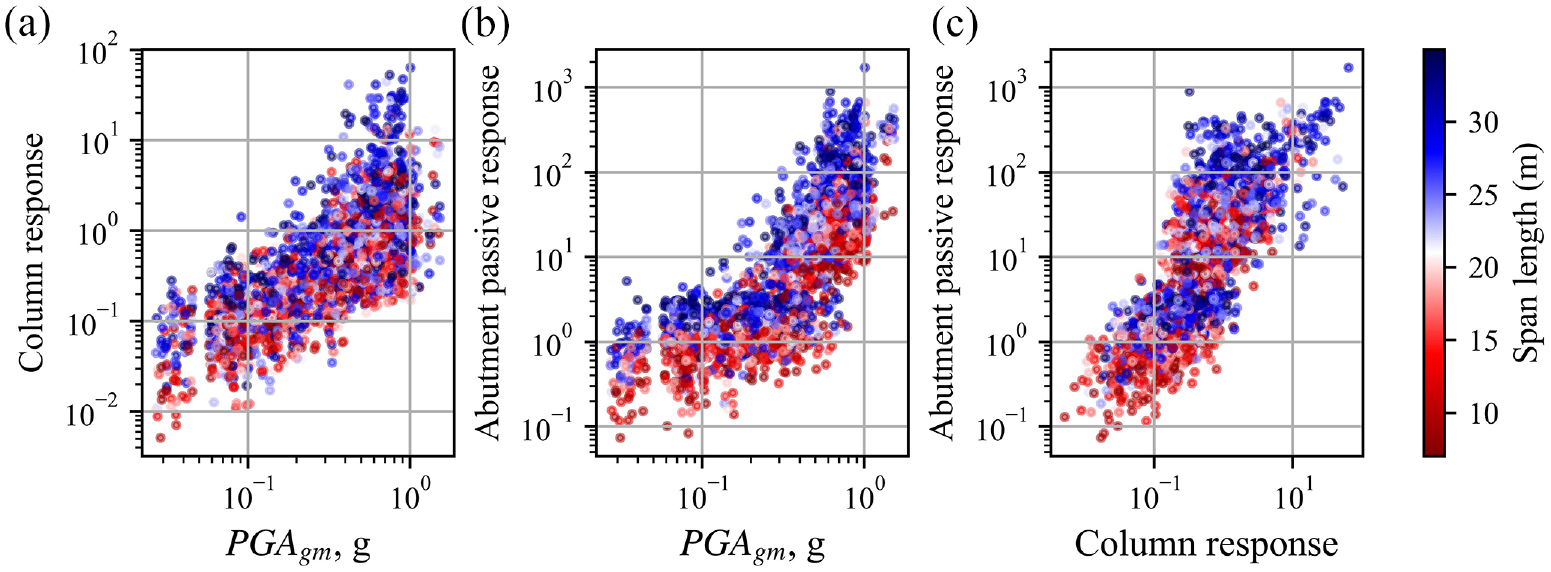
Relationship between components responses,
Seismic demand models using traditional methods
As indicated in previous subsections, traditional methods rely on lognormality assumption of the response distribution conditional on the intensity measure. The linear regression model assumes a linear relationship between responses and intensity measure plus a Gaussian noise (in the log-scale). The expected value of the expression in Equation 15 corresponds to the dashed line presented in Figure 4a; the coefficients of the linear regression model are obtained via ordinary least squares solution. The residuals between components’ prediction and analytical model responses are used to obtain the
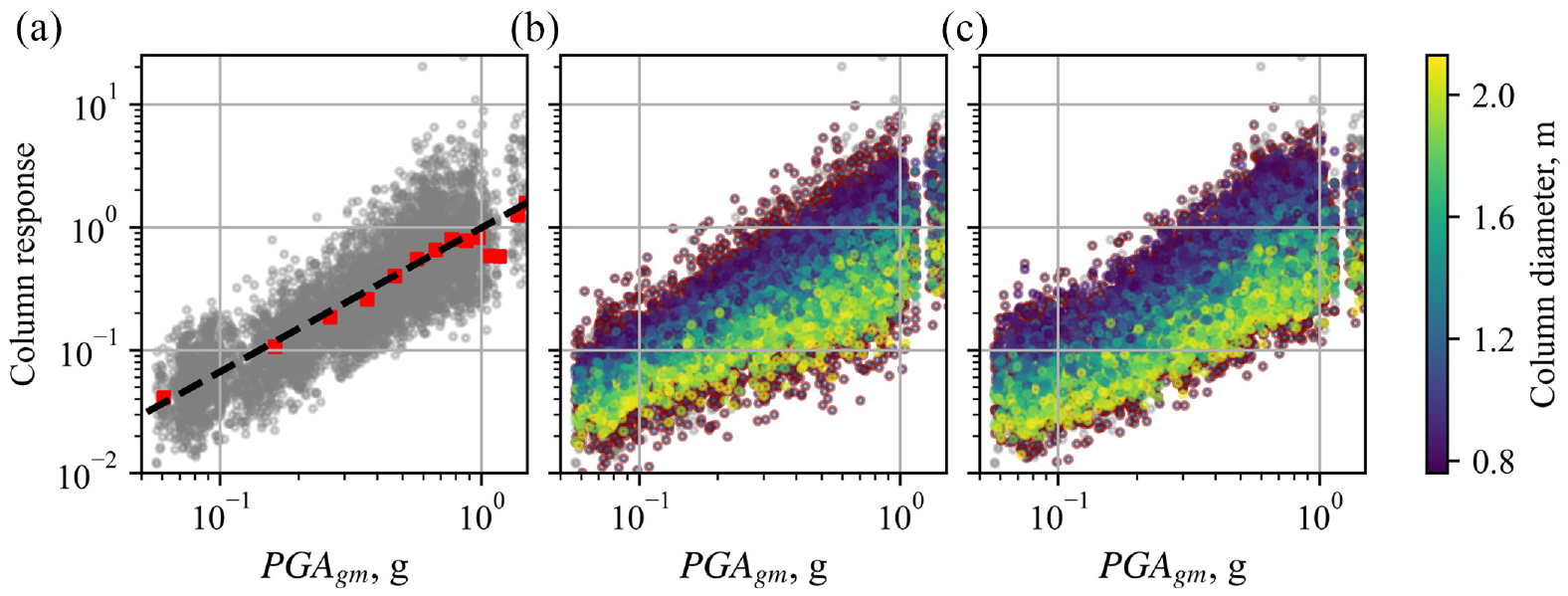
Seismic demands estimated with different approaches for Bridge 3: (a) linear regression, multivariate pdfs and Monte Carlo estimates, (b) univariate surrogate demands based on lasso regression, and (c) multivariate surrogate demands based on kernel ridge regression.
On the contrary, multivariate lognormal distributions fitted at multiple intensity levels allow capturing the variation in the descriptive statistics of the responses at discrete intensity values (shown as red squares in Figure 4a). To obtain such pdfs, the responses are first grouped in bins of 0.1 g, then the within bin component’s responses and associated intensity metric are adjusted following recommendations in (Sudret et al., 2015). That is, the responses of each sample

where
Seismic demand models using ML-based methods
Building the surrogate model entails some steps to assure the model is not trained with ill-conditioned data, does not suffer data leakages, is not overfitting, does not produce inaccurate predictions, among other potential problems. Common good practices include holding out validation sets before any other step is performed, selecting models able to handle collinear predictors, performing standardizing of the data before performing the training process, performing feature selection, among others. A thorough explanation of these steps and common recommendations can be found elsewhere (Du and Padgett, 2020; Ghosh et al., 2013).
For the case study bridges, we used lasso regression and kernel ridge regression methods to develop surrogate demand models. While the former was performed for individual components responses, the latter used simultaneously the eight components’ responses, termed as univariate and multivariate surrogates, respectively. In contrast to the lasso model, the kernel ridge regression model maps the original data set into a high-dimensional space where the interaction between observations depends on the (kernelized) distance between them. Hence, this model is considered more complex than the lasso regression and prone to overfitting. However, both models use regularization seeking to avoid overfitting and for handling collinearities (Vu et al., 2015). The model parameters (or hyperparameters) of these models correspond to a regularization term
The mean predictions (
One-parameter and parameterized fragility models
The demand estimation modeling performed above produces the vector of responses
Typical one-parameter fragility expressions can be obtained from the parameterized fragilities if one plugs the set of parameters

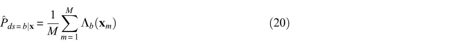
Figure 5 presents the obtained fragilities for Bridges 1 and 3, for all the above-mentioned methods (listed in Table 2), depicting the variation in model performances. Differences among the obtained fragilities are exacerbated as the damage state increases. While Bridge 1 seems to be fairly represented by most of the models, Bridge 3 shows large differences between the benchmark Monte Carlo model and the rest of the approaches (especially the archetype fragility).
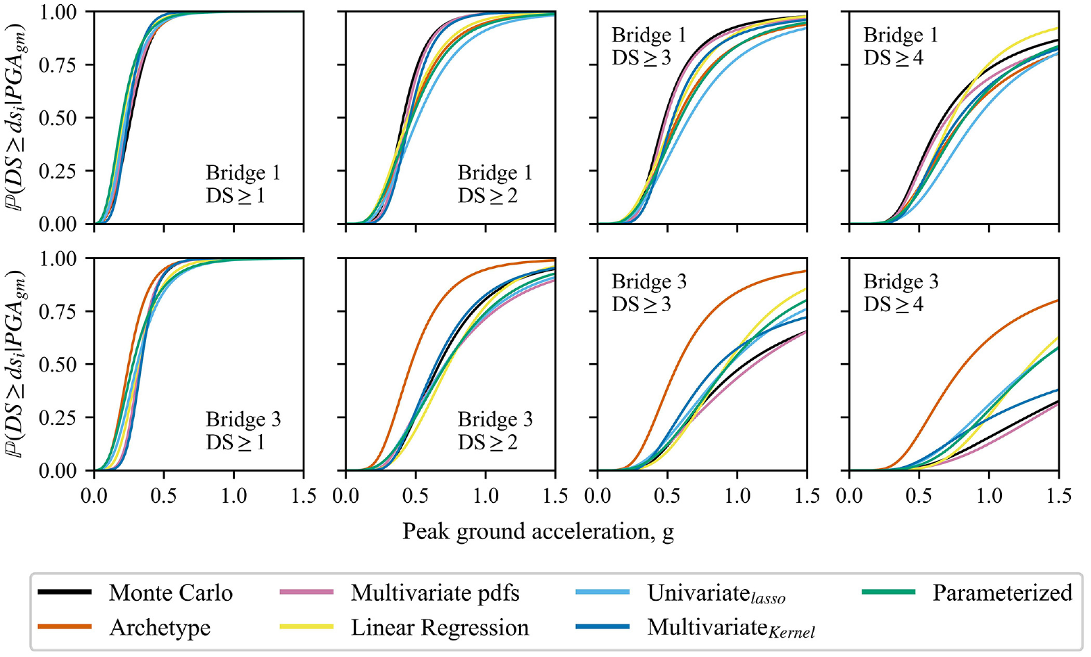
Fragility functions obtained for Bridges 1 (upper) and 3 (lower) for damage states slight to complete.
Design of experiments for different fragility types
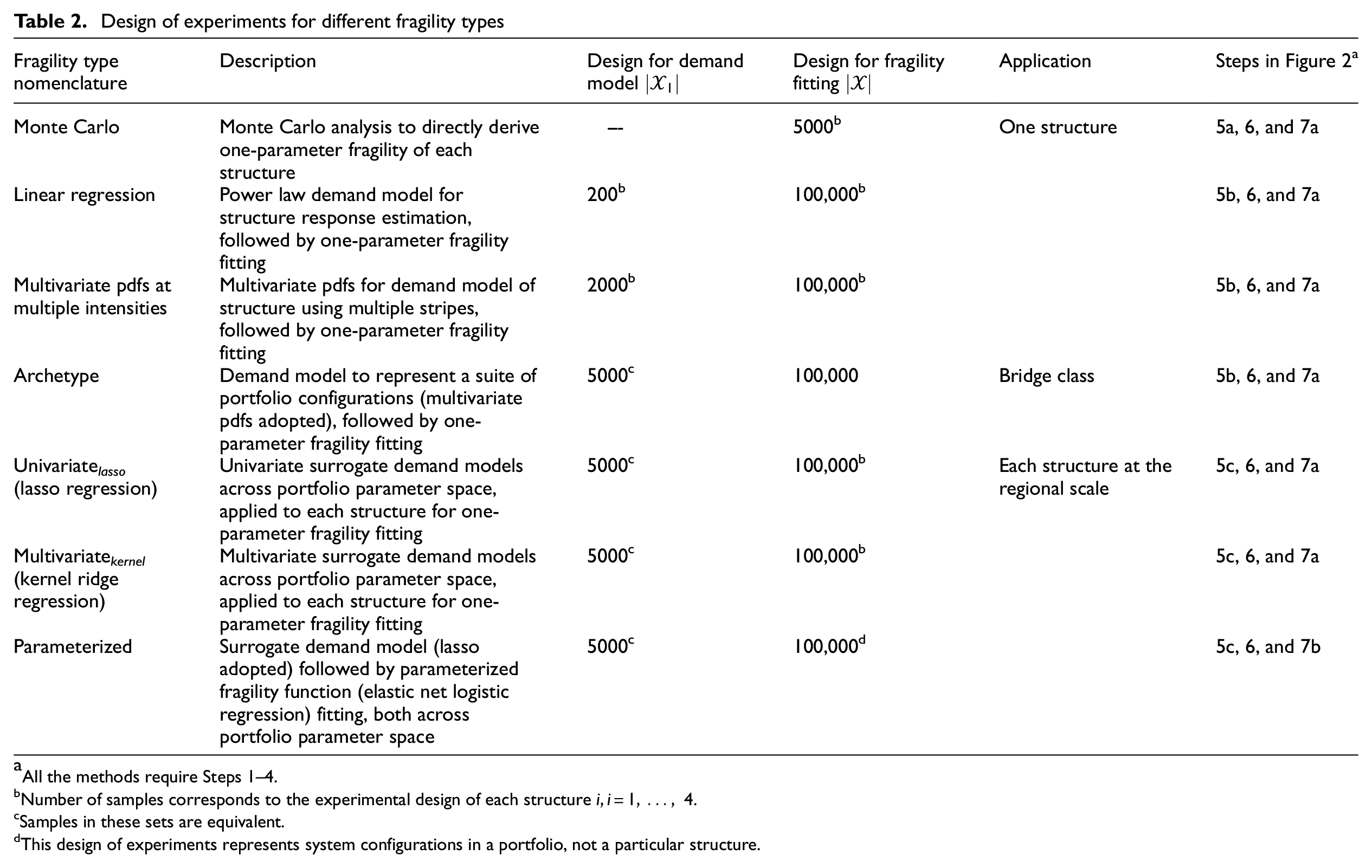
All the methods require Steps 1–4.
Number of samples corresponds to the experimental design of each structure
Samples in these sets are equivalent.
This design of experiments represents system configurations in a portfolio, not a particular structure.
Statistical differences among derived functions
Visual comparison of fragility functions lacks objectivity and does not allow conclusions to be drawn about the appropriateness of a derivation technique. Hence, the methods to measure differences between cdfs or pdfs explained before are adopted herein. The three different statistical distances are computed separately for each method in Table 2, the four damage states and the four bridges under analysis, using the Monte Carlo fragilities as the benchmark model. Figure 6 shows such statistical distances and reveals the fragility models that are closer to the benchmark models, as is the case for the multivariate surrogate (kernel ridge regression) and the multivariate pdfs at multiple intensities (traditional) methods. Linear regression, univariate surrogate (lasso regression), and parameterized fragilities presented slightly larger distances compared to the two previous methods. Finally, the archetype fragility diverges the most from the benchmark model, especially for the fourth damage state.
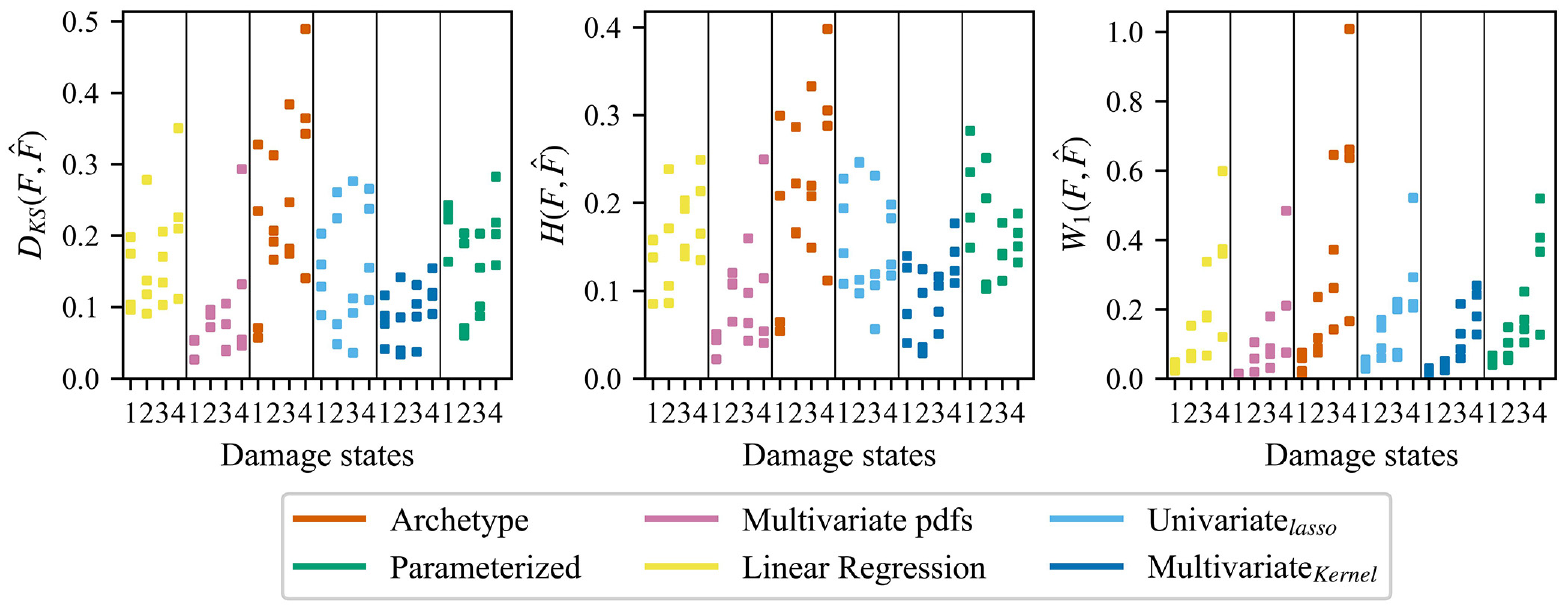
Statistical distances for each fragility derivation method per damage state: 1 slight, 2 moderate, 3 extensive, and 4 complete. Each dot represents one of the four bridges. The boxes in the x-axis represent each of the demand modeling methods evaluated.
The Kolmogorov–Smirnov statistic
Risk estimates at the structural and regional scale
The small-to-large differences found in fragilities derived through different practices should be positioned in terms of its influence on subsequent risk and resilience analyses. In this section, we focus on performance measures related to risks at the structure and regional or portfolio scale.
Risk estimates at the bridge level
The four individual structures previously analyzed are assumed to be part of the highway bridge network presented in Figure 7a; the location of the four bridges is portrayed with blue dots. The bridge network consists of 130 bridges, hypothetically placed in the Memphis Metropolitan and Statistical Area (MMSA) highway system. For illustrative purposes, the area is subjected to earthquakes produced by a point-source located at 35.927 N, 89.919 W. The event magnitude is assumed to follow a truncated Gutenberg–Richter model with
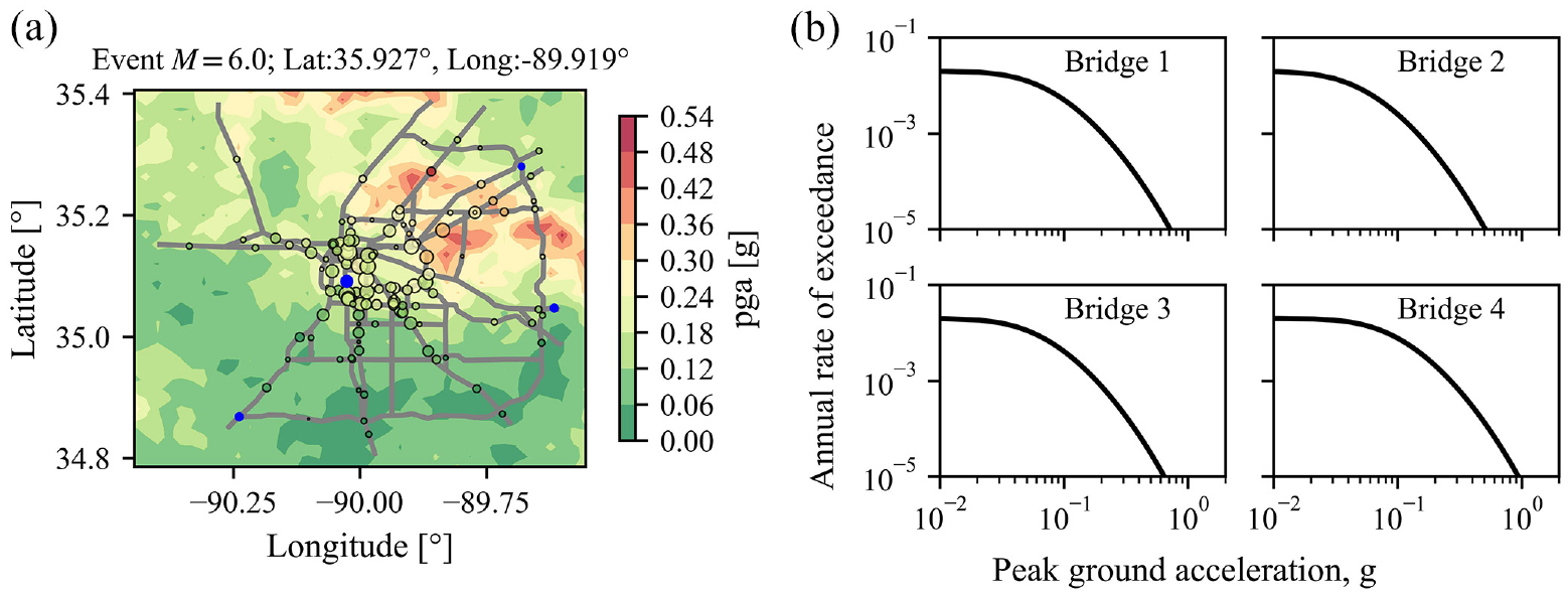
Illustrative example of a highway bridge network subjected to seismic events: (a) network of bridges and (b) mean hazard curves for Bridges 1–4.
The first comparison can be performed in terms of the expected relative loss conditional to the hazard intensity,
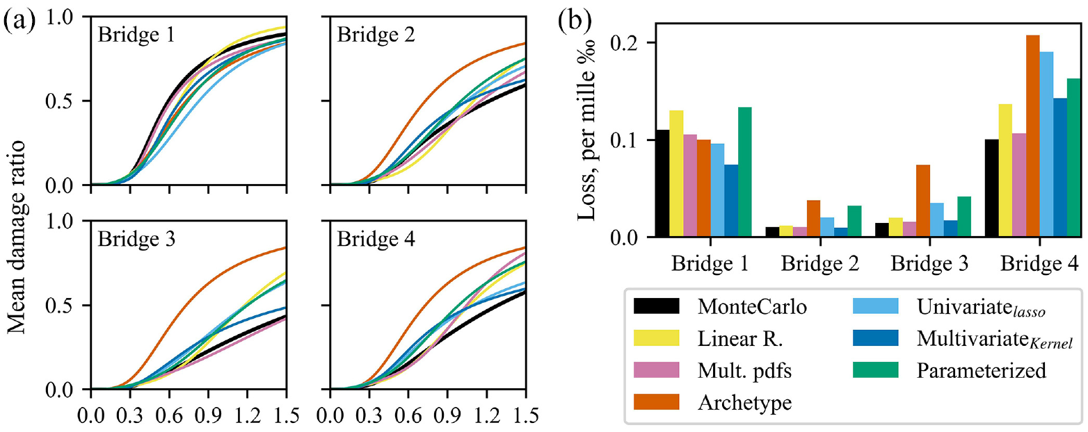
Mean damage ratio curves (a) and relative expected annual losses at the structure level (b).
Another risk metric of interest is the relative expected annual losses (EALs), obtained from Equation 9. The differences that arise in these values between methods (presented in Figure 8b) may be somewhat counterintuitive. For example, in Bridge 4, larger differences are observed between the vulnerability curves of traditional methods (yellow and pink curves) with respect to the benchmark model (black line), compared to those observed for the surrogate-based models (blue curves). However, the relative EAL in the traditional methods resulted closer to the benchmark estimation. This is explained by the fact that lower intensity values are the actual contributors toward the EAL, diminishing the effect of observable differences that occur in higher intensity measures. Overall a similar order of magnitude is obtained between the different approaches, possibly attributed to using probability weighting to compute the EALs.
Risk estimates at the portfolio scale
The seismic hazard at the regional scale is modeled using simulation-based approaches to consider spatially correlated intensities; the correlation model for PGA values used in this study corresponds to the proposed by Jayaram and Baker (2009). The same set of residual samples was kept during the comparisons to guarantee that differences measured are only a product of the differences in fragility models. An example of a simulated scenario for a magnitude
Given the infeasibility of traditional methods to scale up to big portfolios, the three traditional approaches (Monte Carlo, multivariate pdfs for different intensity levels, and linear regression) are disregarded from the subsequent analysis. Archetype fragilities are kept as they are commonly used in regional-scale analysis, and fragility functions for each system configuration are computed using the surrogate-based models (both, demand-driven and fragility-driven approaches). The lasso regression model is termed in the subsequent analyses as surrogate-based model. Thus, the remainder of this article presents a comparison between archetype, surrogate-based (lasso model), and parameterized models.
To estimate the influence of fragility modeling practices at the regional scale, earthquakes with varying magnitude are simulated to estimate the conditional portfolio loss
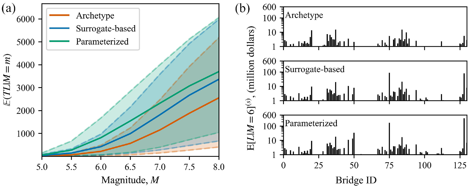
Portfolio risk outcomes: (a) conditional portfolio total losses and (b) average bridge losses for an earthquake
From Figure 9a, the surrogate-based models present slightly closer portfolio loss estimates (solid lines) between them than compared against archetype-based estimations. This similarity, however, does not yield very similar expected annual portfolio losses
Estimation of implications at the network scale
We further investigate the impact of differences in fragility estimates by considering the interaction of bridge functionality within the transportation network. In this study, a bridge that reaches or exceeds moderate damage state,
The fragility functions are used in this stage to estimate the probability of the edge’s failures (i.e. reaching or exceeding moderate damage state), then the edge state (functional or not) is sampled. Therefore, having different fragility derivations primarily impacts the different sampled network conditions. After computing the network event conditions, the idle and recovery sampled times are assigned only to those bridges that lost functionality. Subsequently, the scheduling is defined according to the number of crew members and order of priority predefined for repair purposes (if any). The network time-dependent functionality trajectories are constructed using the scheduled repair times. Every instant
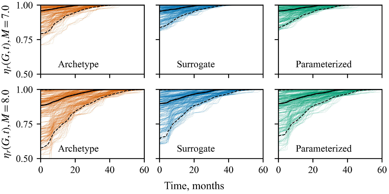
Time-dependent network functionality trajectories using three fragility input models for events with
Comparison of all the recovery trajectories simulated for earthquakes of magnitude
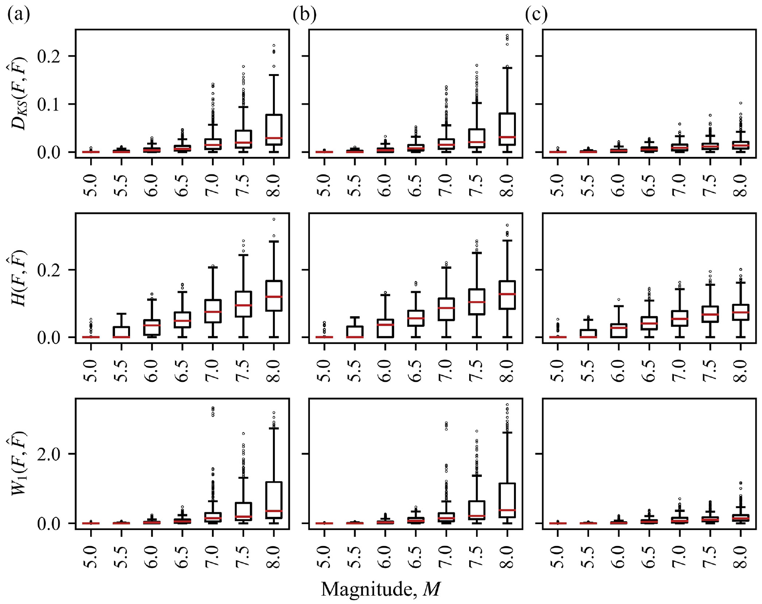
Statistical distances between network recovery trajectories. The boxes arranged in vertical columns represent pair-wise comparison between (a) archetype versus surrogate univariate model, (b) archetype versus parameterized fragility, and (c) surrogate univariate model versus parameterized fragility.
The distances are measured for each pair of methods as a function of the magnitude of the event (shown in Figure 11). The distances measured confirm the relationship between the magnitude and the statistical distances observed previously. As the magnitude increases, the statistical distance also increases between any pair of methods, especially for the archetype-based methods. For instance,
In general, differences at this scale are quite small compared to the vast differences found in risk outcomes at a regional scale. We attribute this to three major factors: (1) the differences between failure probabilities (among derivation methods) only matters at this scale if they produce different network events states and the “distance” itself is not as important as it is when it informs the likelihood of the performance measure (e.g. the conditional relative loss at the structure level); (2) the routes covered by the critical pinpointed bridges in previous stages can be easily replaced by other routes, as it happens on networks with redundant connectivity; and (3) the use of recovery models that do not consider system parameters to predict the individual time to repair (i.e. that act as “archetype” recovery models) hamper the gained granularity of the ML-based fragility models.
Conclusion
This study has targeted the unanswered question of how and if different fragility modeling practices (including traditional and those that leverage emerging surrogate modeling) actually influence seismic risk and resilience quantification. The discussion of fragility derivation approaches centers on (1) the procedures and assumptions of various techniques for demand modeling and (2) the agility of these to yield either one-parameter or parameterized fragility functions, that is, fragilities conditioned on system and/or hazard features. In contrast to existing studies, the implications of fragility techniques are evaluated over performance measures that cut across scales, including from conditional damage probabilities, to expected losses (at the individual and portfolio scale), to network functionality metrics (e.g. recovery trajectories). Case studies using bridges and transportation networks are leveraged to test such implications and systematically contrast their outcomes using posed statistical distance metrics.
Small statistical distances were found between proven traditional methods (for structure-specific fragilities) and ML-based approaches, confirming the ability of the latter to be used for structure-specific analysis with acceptable accuracy. This conclusion extended to estimated risk metrics at the individual structure scale, for example, conditional expected relative losses, where emerging techniques captured particularities on the performance of heterogeneous system configurations. To further support these findings, a hypothetical highway network consisting of 130 bridges was studied. Outcomes showed that capturing granularities in the individual performance is not only important for capturing subtleties in losses predictions but also it may pinpoint fragile structures within the region that could exacerbate, and dominate, the losses in portfolio analyses. These observations showed that resolution in modeling portfolios could impact the risk outcomes and lead to totally different conclusions, possibly affecting objective investment plans (e.g. retrofitting programs). Regarding network functionality analyses, results showed that divergencies in recovery trajectories are not as dramatically impacted by differences in fragility description as they were for the portfolio losses. At this scale, other modeling choices, such as the estimation of individual recovery time without consideration of system parameters, may reduce the impact of fragility model choice and provides an opportunity for further investigation.
While the systematic comparisons are presented using highway bridge networks, the findings of this study can be generalized to other structures embedded in networked systems. The approach proposed in this study to methodically compare fragility model implications can serve as a basis for future fragility method evaluation, propelling objective quantification of their impacts on risk and resilience pipelines. The use of the proposed statistical distance metrics also promotes comparison of regional-scale performance and resilience measures that keep the heterogeneity of the individual performances (i.e. those that are not based on aggregation), as was shown by comparing individual network recovery trajectories. Overall, the findings of this study suggests that emerging techniques are equipped to go beyond efficient estimations to enable the construction of models of heterogeneous portfolios, better supporting decisions processes that may occur at different scales, space, and time, throughout infrastructure systems.
Footnotes
Declaration of conflicting interests
The author(s) declared no potential conflicts of interest with respect to the research, authorship, and/or publication of this article.
Funding
The author(s) disclosed receipt of the following financial support for the research, authorship, and/or publication of this article: The authors acknowledge the support provided by the National Science Foundation under Award Number CMMI-2227467. The first author acknowledges the grant support from the Fulbright-Minciencias scholarship program. Any opinions, findings, conclusions, or recommendations expressed in this material are those of the authors and do not necessarily reflect the views of the National Science Foundation or the Fulbright-Minciencias program.