Sage Journals: Discover world-class research

Abstract

Cone penetration tests (CPTs) are a commonly used in situ method to characterize soil. The recorded data are used for various applications, including earthquake-induced liquefaction evaluation. However, data recorded at a given depth in a CPT sounding are influenced by the properties of all the soil that falls within the zone of influence around the cone tip rather than only the soil at that particular depth. This causes data to be blurred or averaged in layered zones, a phenomenon referred to as multiple thin-layer effects. Multiple thin-layer effects can result in the inaccurate characterization of the thickness and stiffness of thin, interbedded layers. Correction procedures have been proposed to adjust CPT tip resistance for multiple thin-layer effects, but many procedures become less effective as layer thickness decreases. To compare or improve these procedures and to develop new ones, it is critical to have pairs of measured tip resistance (q^m) and true tip resistance (q^t) data, where q^m is the tip resistance recorded by the CPT in a layered profile, and q^t represents the tip resistance that would be measured in the profile absent of multiple thin-layer effects. Unfortunately, data sets containing q^m and q^t pairs are extremely rare. Accordingly, this article presents a unique database containing laboratory and numerically generated CPT data from 49 highly interlayered soil profiles. Both q^m and q^t are provided for each profile. An accompanying Jupyter notebook is provided to facilitate the use of the data and prepare them for future statistical learning (or other) applications to support multiple thin-layer correction procedure development.

Keywords

Multiple thin-layer effects CPT cone penetration test liquefaction material point method calibration chamber

Introduction

The cone penetration test (CPT) is a widely used in situ geotechnical method for characterizing soil profiles for a variety of applications, including earthquake-induced soil liquefaction evaluations. Parameters that may be obtained from the CPT include tip resistance (q_c), sleeve friction (f_s), and pore pressure (u₂), each recorded typically at 0.01 m to 0.05 m depth increments. Tip resistance recorded at a particular depth is affected by the properties of all the soil that falls within the zone of influence around the tip of the cone, not just the properties of the particular soil at the current cone depth. Since the zone of influence for q_c can be between ∼10 and 30 times the diameter of the cone (e.g. Ahmadi and Robertson, 2005), it is difficult to identify the exact depths of layer boundaries and accurately characterize the q_c of individual soil layers in highly stratified soil profiles. This is illustrated in Figure 1, where a CPT performed in a homogeneous clay or sand profile records a characteristic or “true” tip resistance (designated as q^t_clay or q^t_sand), but a CPT performed in a clay profile with a thin embedded sand layer records a “measured” tip resistance profile (designated as q^m) that (1) smears the boundaries of the embedded layer and (2) underestimates the tip resistance in the embedded layer. When many thin layers occur in sequence in a profile, these effects are amplified and are referred to as “multiple thin-layer effects.” Multiple thin-layer effects have detrimental consequences on engineering predictions that rely on correlations with CPT data. For example, the widespread over-prediction of liquefaction severity in Christchurch, New Zealand, for complex, highly interlayered soil profiles is partially attributed to this phenomenon (e.g. Boulanger et al., 2016; Cox et al., 2017; McLaughlin, 2017; Maurer et al., 2014; Yost et al., 2019).

Figure 1.

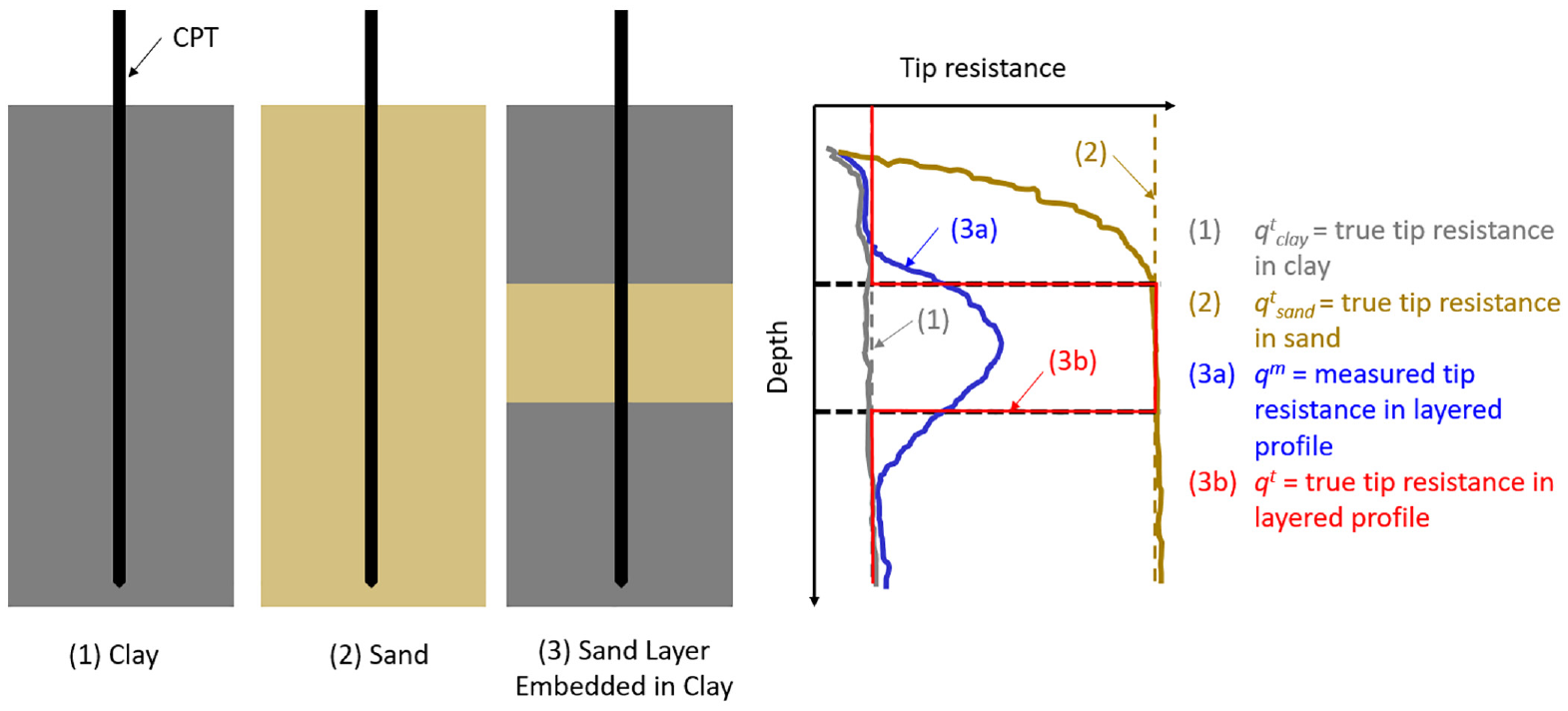
Schematic of multiple thin-layer effects in CPT data. Tip resistance from CPTs performed in homogeneous clay and sand profiles can be considered characteristic or “true” tip resistances, q^t_clay (labeled 1) and q^t_sand (labeled 2). Measured tip resistance (q^m) from a CPT performed in a layered sand–clay profile is affected by multiple thin-layer effects (labeled 3a). True tip resistance of the layered profile (q^t, labeled 3b) can be constructed using q^t_sand, q^t_clay, and the known profile geometry. CPT: cone penetration test.

Recently, several automated procedures have been proposed to correct for multiple thin-layer effects (e.g. Baziw and Verbeek, 2022; Boulanger and DeJong, 2018; Cooper et al., 2022; de Greef and Lengkeek, 2018; Yost et al., 2021) and to detect layer boundaries from CPT data (e.g. Hudson et al., 2023; Molina-Gómez et al. 2022). Generally, multiple thin-layer correction procedures take the recorded or measured tip resistance (q^m) as an input (e.g. the profile labeled 3a in Figure 1) and output an estimate of the true tip resistance (q^t) (e.g. the profile labeled 3b in Figure 1). If the procedure follows a forward model, it directly applies a set of correction factors to q^m, outputting a “corrected” tip resistance (q^corr). If the procedure follows an inverse model, an “inverted” tip resistance (q^inv) is guessed to estimate q^t, and a model describing the blurring process of cone penetration is applied to q^inv to obtain a simulated measured tip resistance (q^m,sim). Then, q^m,sim is compared with the recorded q^m. If the misfit between q^m,sim and q^m is too large, the procedure iterates to improve q^inv. A flowchart summarizing the types of procedures is shown in Figure 2.

Figure 2.

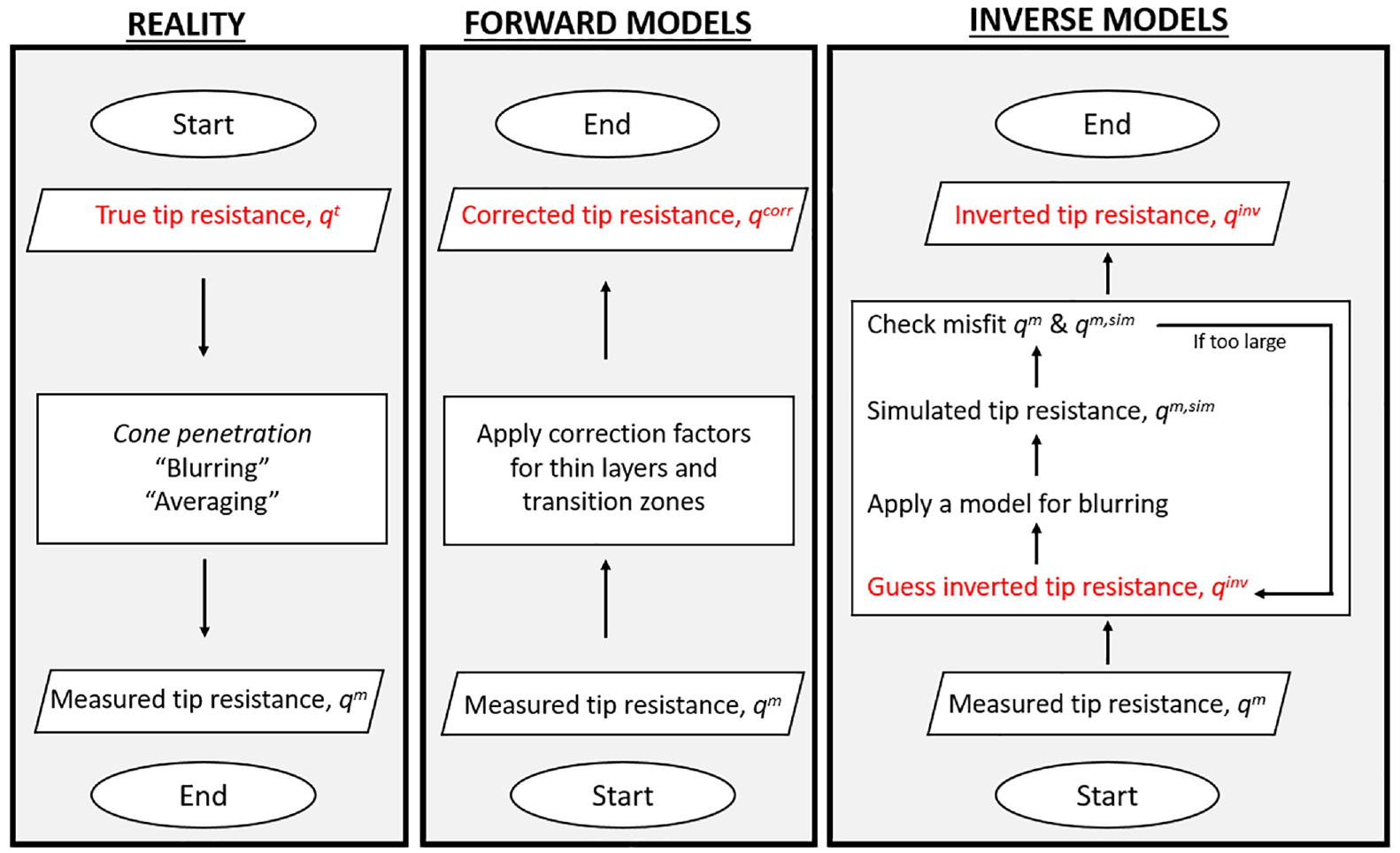
Flow chart describing forward and inverse multiple thin-layer correction procedures.

Existing multiple thin-layer correction procedures have several shortcomings, including:

Procedures must be calibrated and validated with profiles that include both q^m and q^t. While q^m data are readily available, obtaining the corresponding q^t is more difficult because soil profile geometry and soil properties for each layer must be known. For example, field CPT data in layered profiles only provide q^m, not q^t. To obtain sets of q^m and q^t, laboratory calibration chamber tests, numerical simulations of CPTs, or empirical correlations may be used. However, large sets of paired q^m and q^t data are not readily available in the literature.

Indirect assessment of the efficacy of multiple thin-layer correction procedures can be performed using field data. For example, Yost et al. (2021) applied multiple thin-layer correction procedures to a CPT database from Christchurch, New Zealand, and compared the accuracy of liquefaction evaluations performed with corrected and uncorrected data. However, they found no improvement in the accuracy of liquefaction evaluations using the corrected data from any of the correction procedures. Furthermore, even if an improvement was observed, it would not necessarily mean that the procedure accurately corrected the data. Direct assessment with q^m and q^t pairs is required as a first step in evaluating the efficacy of these procedures.

Many existing procedures become ineffective in soil profiles with layer thicknesses of about 1.6 times the diameter of the cone (d_cone) or smaller, as shown in the work by Yost et al. (2021, 2022b). As the layers become thinner, their contribution to q^m becomes smaller, and ultimately, it may be impossible to visually identify the presence of very thin layers in a q^m profile. Many multiple thin-layer correction procedures rely on the ability to identify peaks and troughs in q^m (e.g. the Deltares procedure from Yost et al., 2021), or use the rate of change in q^m or another CPT parameter (e.g. Boulanger and DeJong, 2018), to identify layer boundaries. As the CPT data in layered zones become increasingly smoothed due to smaller layer thicknesses, these procedures become less effective. Many profiles of interest have layers less than 1.6d_cone thick, which require new or improved procedures that can account for layers of this thickness. For example, layer thicknesses on the order of centimeters were observed in the Christchurch data based on high-quality soil samples. However, CPT data in these profiles were collected using 10 cm² (d_cone = 3.6 cm) and 15 cm² (d_cone = 4.4 cm) cones, meaning layers with thicknesses less than 5.8 cm to 7.0 cm are unlikely to be identified using existing multiple thin-layer correction procedures.

In addition to layer thickness, the stiffness contrast between soil layers impacts the severity of multiple thin-layer effects. Unlimited combinations of stiffness contrast between loose/soft and dense/stiff layers in a profile present challenges to correction procedures. Many previous laboratory and numerical studies of multiple thin-layer effects only consider specific stiffness ratios, making it difficult to extrapolate results to other conditions (e.g. as discussed by Yost et al., 2022b). Although the Boulanger and DeJong (2018) procedure is capable of correcting data with any stiffness contrast, centrifuge testing by Khosravi et al. (2022) showed that the procedure tended to overpredict tip resistance in a thin dense sand layer embedded in a clay (larger stiffness ratio), and underpredict tip resistance in a thin loose sand layer embedded in a clay (smaller stiffness ratio). The creation of a database containing many stiffness ratios will support the development of more effective correction procedures.

A salient feature of inverse-style correction procedures such as Boulanger and DeJong (2018) and Cooper et al. (2022) is that they must define how the CPT blurs or filters q^t to obtain the q^m that is actually recorded. This blurring process is a complex physical procedure not well captured by current models (Cooper et al., 2022). Some existing approaches use a blurring filter consisting of a truncated chi-square distribution with depth-dependent weighting factors (i.e. Boulanger and DeJong, 2018), or a simplified version of this distribution (i.e. Cooper et al., 2022). A filter that accurately describes the physics behind multiple thin-layer effects will, when applied to a q^t profile, produce a q^m,sim profile that closely matches the actual q^m profile. To develop and assess how well a blurring filter works, pairs of q^m and q^t data are required.

Correcting CPT data in highly stratified profiles with procedures that do not perform well is, at best, ineffective and, at worst, unconservative. In some cases, application of these procedures can result in an over-simplified profile that smooths over potentially critical information. All the while, the end user may be tempted to accept the smoothed profile as-is because the data appear to be “cleaned up.” It is, therefore, critical to thoroughly understand and vet correction procedures before use. To overcome the shortcomings of existing procedures described previously and support the development and quantitative validation of new ones, a combined laboratory and numerical database has been constructed containing CPT data from 49 highly interlayered soil profiles with embedded layer thicknesses ranging from 0.01 m to 0.08 m (0.4d_cone to 3.1d_cone). Each profile has both q^m and q^t data. The data are presented in an array structure that can easily be added to and manipulated as desired by the researcher. The following sections describe the creation of this database. First, the development of the laboratory and numerical parts of the CPT database is discussed. Then, details are provided on how to access, supplement, and utilize the database. Some examples of how this database can be used to assess blurring filters and the efficacy of existing multiple thin-layer correction procedures are presented. Finally, the limitations and nuances of this database are discussed.

Development of CPT database

Laboratory data

A portion of the database presented in this article was generated using curated and processed CPT data originally collected in a series of calibration chamber tests performed by De Lange (2018). These laboratory tests were also used to calibrate the numerical model used to produce the numerically generated portion of this database. The following sections provide an overview of the laboratory tests and describe how the data were processed to create the q^m and q^t profile pairs provided in this database.

Overview

A large CPT calibration chamber study was performed by De Lange (2018) to study multiple thin-layer effects. The calibration chamber consisted of a series of stacked cylindrical rings with an inner diameter of 0.9 m and a height of approximately 1 m. Soil profiles were prepared inside the chamber. A pressurized, water-filled cushion placed on top of the soil profile provided overburden pressure, and ports within the cushion allowed CPTs to be advanced through the soil profile. Drainage was allowed through a geotextile and filter plate at the bottom of the chamber and through the ports in the cushion at the top of the chamber. The radial boundary was rigid, as discussed by Yost et al. (2023).

Both homogeneous and highly interlayered soil profiles were constructed in the chamber. Each profile was designated with a “Soil Model” number ranging from 1 to 10. Multiple CPTs were advanced in each soil profile, typically with sequentially increasing applied overburden pressure. Only CPTs performed with a 25-mm-diameter cone were included in this database (CPTs performed in Soil Model 6 and Soil Model 7 used 36-mm-diameter cones and were, therefore, excluded). Two homogeneous sand profiles (Soil Model 1 and Soil Model 5) were used as reference models. Three CPTs were performed in Soil Model 1 (at 25, 50, and 100 kPa), but the 25 kPa test was excluded herein because of experimental artifacts in the data. Three CPTs were performed in Soil Model 5, each at 100 kPa. However, Yost et al. (2023) showed that the measurements recorded by the second and third CPTs in this Soil Model were affected by densification and stress changes caused by the previously advanced CPTs. Thus, only the measurements from the first CPT are included herein. The three reference CPTs performed in the homogeneous profiles are summarized in Table 1.

Table 1.

Summary of laboratory CPTs performed in homogeneous sand profiles (used as reference models)

Reference CPT number	De Lange (2018) soil model number	Applied overburden stress, σ’_v (kPa)	Relative density, D_R, of sand layers (%)
1	1	50	36
2	5	100	60
3		100

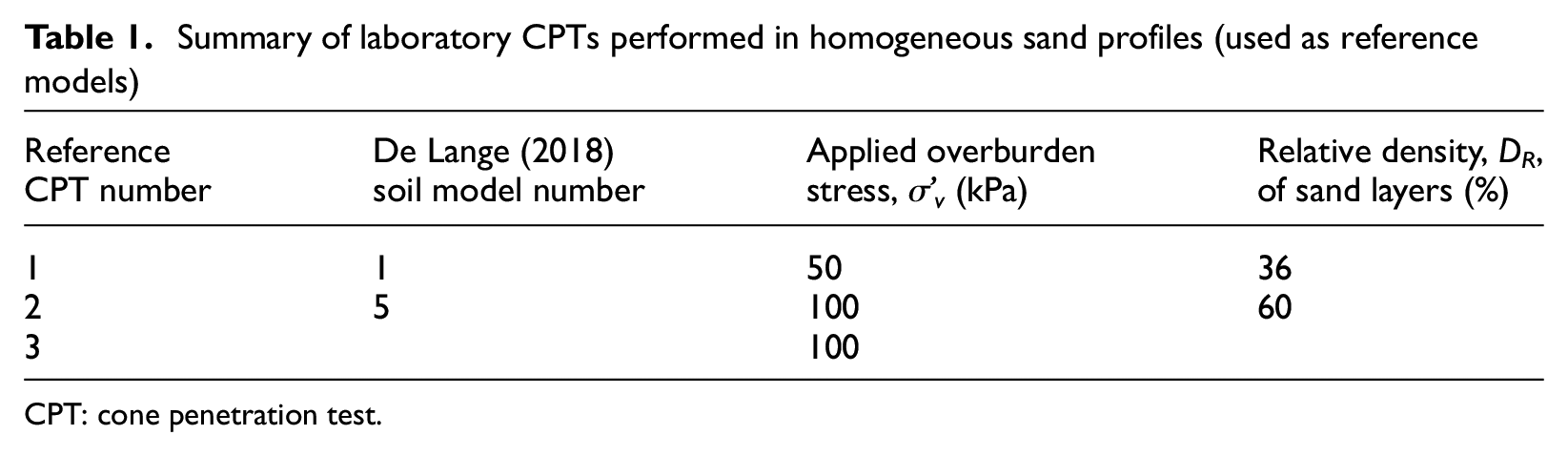
CPT: cone penetration test.

Data from the remaining layered profiles (Soil Models 2 through 4 and 8 through 10), as well as one profile from the start-up phase of the experiments (Soil Model 4—Start Up), were used to compile the laboratory portion of the database (see soil profile geometries in Figure 3). In total, there were 19 CPT soundings performed in layered profiles whose tip resistance data could be used as q^m. The relevant information for each of those soundings is summarized in Table 2. Note that the tip resistance data from De Lange (2018) were digitized and then resampled at 0.001 m depth increments, consistent with the sampling intervals used during the laboratory tests.

Figure 3.

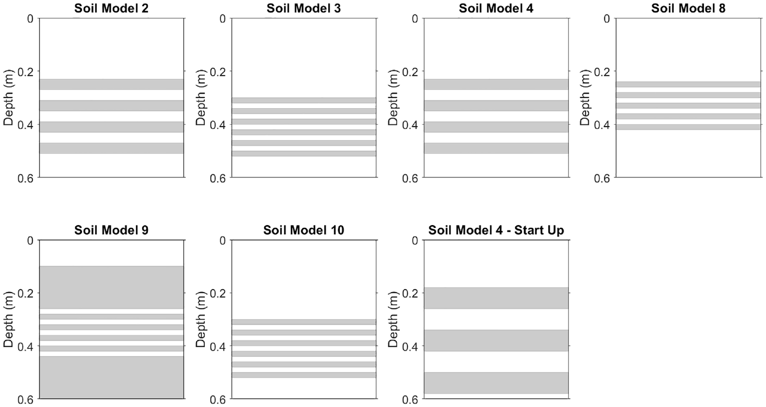
Layered soil profile geometries from the De Lange (2018) laboratory experiments. Gray areas represent clay layers, and white areas represent sand layers. Note that soil profiles extend to ∼1 m, but only the interlayered zones are shown here.

Table 2.

Summary of the CPTs performed in layered sand–clay profiles composing the laboratory portion of this database

Laboratory database CPT number	De Lange (2018) soil model number	Applied overburden stress, σ’_v (kPa)	Relative density, D_R, of sand layers (%)	Undrained shear strength, s_u, of clay layers (kPa)
1	2	25	29	23.8
2	2	50	29	27.9
3	3	25	28	23.8
4		50		27.9
5		100		37.9
6	4	25	54	23.8
7		50		27.9
8		100		37.9
9	8	25	61	23.8
10		50		27.9
11		100		37.9
12	9	50	28	27.9
13	9	100	28	37.9
14	10	10	18	19.8
15		20		21.9
16		30		24.0
17	4—Start Up	25	31	23.8
18		50		27.9
19		200		60.4

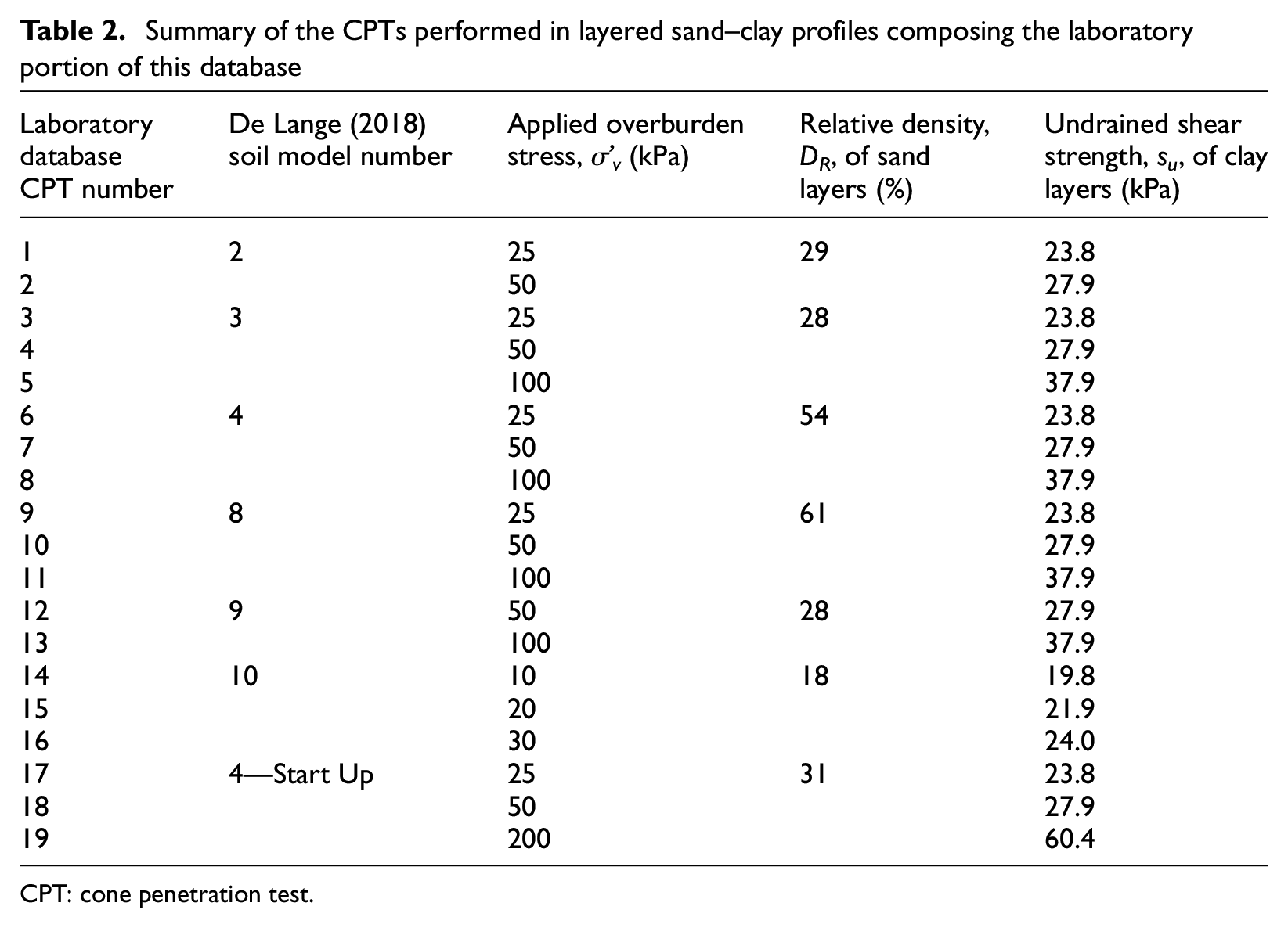
CPT: cone penetration test.

To construct q^t profiles that correspond to each of the q^m profiles, q^t_sand and q^t_clay are determined for each combination of sand relative density (D_R), clay undrained shear strength (s_u), and applied vertical effective stress (σ’_v) detailed in Table 2. All data are normalized for overburden pressure to obtain dimensionless values. Then, q^t_sand and q^t_clay are used in conjunction with the profile geometry to define a q^t that corresponds to each q^m. The procedure is summarized in the flowchart in Figure 4 and detailed in the following sections.

Figure 4.

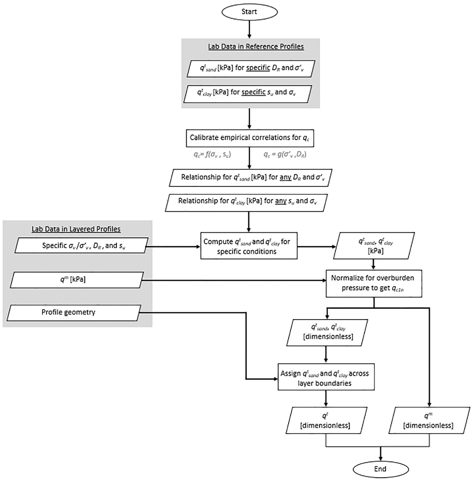
Flowchart for obtaining normalized q^m and q^t pairs from laboratory data.

Determining tip resistance from overburden pressure and density for sands

An empirical relationship was adopted to compute q^t_sand from any D_R and overburden pressure. It was calibrated with the CPT data collected in the reference profiles from Table 1. The empirical relationship was required for two reasons: (1) The D_R and overburden pressure associated with each CPT performed in the layered profiles did not necessarily match the D_R and overburden pressure associated with the three CPTs performed in the homogeneous profiles. Therefore, data collected in the homogeneous profiles could not be used directly to get q^t_sand in the layered profiles; (2) the layered sand–clay profiles did not contain sand layers thick enough to confidently establish a q^t_sand for that specific D_R and overburden pressure.

Thus, the following equation from Schmertmann (1978) was used to relate q_c to D_R in sands:

D_{R} = \frac{1}{C_{2}} \ln (\frac{q_{c}}{C_{0} σ'^{C_{1}}})

(1)

where C₀, C₁, and C₂ are coefficients selected to fit the data; σ’ is assumed to be the vertical effective stress (σ’_v) for normally consolidated sands; q_c and σ’ are in kPa; and D_R is in decimal form. Because we are interested in estimating q_c from D_R, Equation 1 can be rewritten as:

q_{c} = C_{0} σ'_{v}^{C_{1}} \exp (C_{2} D_{R})

(2)

C₀, C₁, and C₂ were determined from a nonlinear regression analysis (using Matlab function fitnlm) using data from the CPTs performed in the homogeneous sand profiles. For each reference CPT in Table 1, q_c and σ’_v were averaged between 0.1 and 0.7 m. D_R for these profiles was known (shown in Table 1), and the coefficients were computed as C₀ = 45.568, C₁ = 1.0103, and C₂ = 1.1702. Because there were only three data points available, it was possible to perfectly fit the data (R² = 1), but note that these results would be expected to be more reliable if more data points are included in future analyses, despite the anticipated reduction in R². The laboratory and predicted q_c values are compared in Table 3.

Table 3.

Comparison of tip resistance (q_c) measured in the laboratory tests in homogeneous sand profiles and q_c computed using Equation 2

Reference CPT number	Relative density, D_R (%)	Average vertical effective stress, σ’_v (kPa)^a	Average measured q_c (MPa)^a	Computed q_c (Mpa)
1	36	53.7	3.88	3.88
2	36	103.7	7.55	7.55
3	60	103.8	10.0	10.0

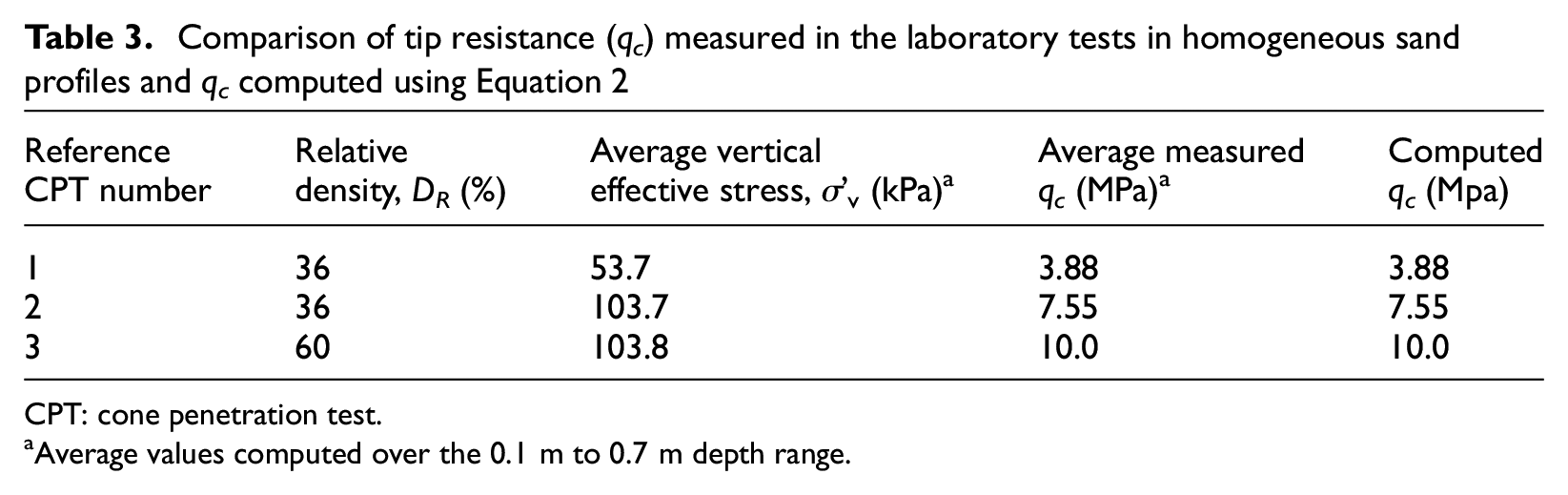
CPT: cone penetration test.

Average values computed over the 0.1 m to 0.7 m depth range.

Determining tip resistance from overburden pressure and undrained shear strength for clays

An empirical relationship calibrated with the calibration chamber data was also adopted to compute q^t_clay from any undrained shear strength (s_u) and overburden pressure. For the undrained conditions expected during cone penetration in the clay layers, q_c can be related to s_u by:

q_{c} = N_{k} s_{u} + σ_{v}

(3)

where N_k is the cone factor; σ_v is the total vertical stress; and all other variables are as previously defined. Since no reference clay profiles were included in the De Lange (2018) study, the relationship between q_c and s_u was established using data from Soil Model 4—Start Up, a layered profile with 7-cm-thick clay layers. Note that these layers are approximately 2.8 times the thickness of the cone diameter, which was shown by Yost et al. (2022b) to be large enough to obtain a “true” tip resistance in a soft layer embedded in stiffer soil. The minimum q_c measured in the shallowest clay layer and the corresponding σ_v were recorded and used for the regression analysis (see Table 4). The R² value of the regression is 0.983. The resulting N_k is 9.9519, which falls within the range of N_k values reported in the literature for similar soft clays (9.3 to 11.5 according to Ceccato et al., 2016b), and is close to the 10.4 that was computed by De Lange (2018) using data from a different study on the same clay.

Table 4.

Comparison of tip resistance (q_c) measured in the laboratory tests in thick clay layers and q_c computed using Equation 3

Laboratory database CPT number	Undrained shear strength, s_u (kPa)	Total vertical stress, σ_v (kPa)^a	Measured q_c (kPa)^a	Computed q_c (kPa)
17	23.8	29.5	277	267
18	27.9	54.5	375	332
19	63.4	204.4	782	806

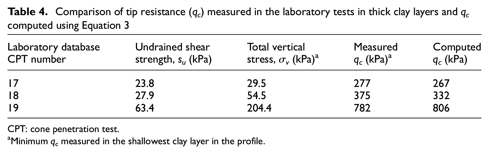
CPT: cone penetration test.

Minimum q_c measured in the shallowest clay layer in the profile.

It is worth mentioning that Soil Model 9 had 16-cm-thick clay layers and q_c measured in those layers could have been included in this regression analysis. However, we excluded these data for two reasons: (1) the degree of consolidation in the 16-cm-thick clay layers is expected to be less than the degree of consolidation in the 2- to 7-cm-thick layers present in the remainder of the soil models; and (2) the drainage conditions for the 16-cm-thick clay layer likely impact the tip resistance, and since pore pressure measurements were not obtained, it is not possible to correct for this.

Normalizing the laboratory data

Once Equations 2 and 3 were used to compute q^t_sand and q^t_clay for each CPT listed in Table 2, the Idriss and Boulanger (2008) approach was used to normalize all tip resistances (i.e. q^m, q^t_sand, and q^t_clay) for overburden pressure:

q_{c 1 n} = (q_{c} / P_{a}) C_{N}

(4)

where q_c1n is normalized cone tip resistance; P_a is atmospheric pressure in the same units as q_c; and C_N is a dimensionless correction factor defined by:

C_{N} = {(P_{a} / σ_{vo}^{'})}^{m}

(5)

where σ’_vo is the initial effective vertical stress in the same units as P_a, and m is computed as:

m = 1.338 - 0.249 {q_{c 1 n}}^{0.264}

(6)

Note that since m depends on q_c1n, the procedure to compute q_c1n is iterative. From here onward, references to q^m, q^t_sand, and q^t_clay are to their normalized (q_c1n) values.

Constructing measured and true tip resistance profiles

The q^m, q^t_sand, and q^t_clay data were truncated between 0.1005 and 0.6005 m to exclude data affected by boundary effects. This eliminated data at the top of the profile where tip resistance is impacted by the upper boundary and not yet fully developed and at the bottom of the profile where results are impacted by the rigid bottom boundary. For each soil profile, q^t was constructed by assigning q^t_sand and q^t_clay over the depths associated with the sand and clay layers, respectively. Note that although this would ideally result in a piecewise constant profile, it is necessary for there to be only one q^t associated with each depth value to align the q^t and q^m profiles for further use. The depths at which the data were sampled (in 0.001 m increments) were realigned (offset by 0.0005 m) such that no data point would fall exactly on a layer boundary. Consequently, the q^t profiles resulting from this procedure slightly underestimate the thickness of each layer by up to 1 mm. The resulting q^m and q^t pairs are shown in Figure 5.

Figure 5.

Pairs of q^m and q^t generated from laboratory data. Clay layers are indicated in gray. Laboratory database CPT number is shown above each plot. Note that soil profiles extend to ∼1 m, but only the interlayered zones are shown here. CPT: cone penetration test.

Assessing efficacy of empirical relationships and uncertainties in laboratory data

As shown in Figure 5, many profiles had relatively thick upper and lower sand layers, although as previously noted, none were thick enough to confidently establish a q^t_sand for that profile. A thickness of at least 12d_cone, or 0.3 m for these profiles, is required according to Yost et al. (2022b) (although this thickness will vary somewhat based on stiffness ratio). Therefore, we would expect the peak value of q^m to be less than q^t in the upper and lower sand layers, and to approach q^t as layer thickness increased. In general, this trend can be observed in Figure 5. However, the efficacy of the regression used to determine q^t_sand is limited by the small amount of data used to calibrate it. For example, we would expect the match between q^t and q^m to be much closer for CPT numbers 14 through 16 since the upper and lower sand layers are so thick. However, these tests were performed with D_R = 18% at overburden pressure of 10 to 30 kPa, well outside the range of values used to calibrate the regression (the closest reference profile was D_R = 36% at 50 kPa). The regression also does not perform as well for CPT numbers 6 through 8, where q^t is computed to be smaller than q^m in the upper and lower sand layers. These CPTs were performed in a profile with D_R = 54%, but q^m was observed to be larger than the q^m measured in the similarly dense reference profile with D_R = 60%. This may indicate that the sand layers were denser than reported.

Uncertainty in the laboratory calibration chamber tests also contributes to unexpected trends in Figure 5. Within a given profile, density of the sand was reported to vary as D_R ± 10%, and this resulted in variations in tip resistance of up to ∼20% from the mean value within a single CPT sounding in the homogeneous profiles (Yost et al., 2023). Variation in actual D_R of the sand will impact the performance of the regression. For example, the regression results in a q^t that is smaller than q^m in the upper sand layer of CPT Number 9, but q^t matches q^m closely in the lower sand layer.

The regression for q^t_clay was calibrated using data from CPT numbers 17 through 19. In the thick clay layers of CPT numbers 12 and 13, q^t_clay is approximately equal to q^m, which is expected. None of the other CPTs had clay layers that were thick enough for q^m to reach q^t_clay; this is captured appropriately with the regression, as evidenced by q^t being less than q^m for all embedded clay layers.

Numerically simulated data

The bulk of the database described in this article consists of data created from high-fidelity numerical simulations of cone penetration in layered profiles using the material point method (MPM). Numerical simulations provide a faster and cheaper alternative to performing laboratory calibration chamber tests; for example, one numerical CPT simulation in this database takes a few days to perform, while a laboratory testing program could take several months. This numerical model was calibrated and validated in previous work by Yost et al. (2022b) using the De Lange (2018) laboratory data detailed in the previous section. The following sections provide an overview of MPM and how the simulations were used to generate q^m and q^t pairs for a variety of soil profile geometries.

MPM background

The MPM is an advanced numerical modeling technique developed by Sulsky et al. (1994) that combines features of mesh-based and particle-based methods. It is well-suited for large deformation problems because it does not suffer from mesh tangling. MPM has been shown to successfully simulate cone penetration in clays (e.g. Beuth and Vermeer, 2013; Bisht et al., 2021a, 2021b; Ceccato et al., 2015, 2016a, 2016b; Ceccato and Simonini, 2017), sands (e.g. Ghasemi et al., 2018; Martinelli and Galavi, 2021, 2022; Tehrani and Galavi, 2018), and layered sand–clay profiles (e.g. Yost et al., 2022a, 2022b, 2023). In this article, the Yost et al. (2022b) framework and geometry are adopted. The MPM model and the calibration procedure are thoroughly explained in the work by Yost et al. (2022b) and thus are only briefly described here. It was shown by Yost et al. (2022b) that three MPM simulations could successfully generate a q^m and q^t pair for a layered soil profile with two material types. Namely, one simulation performed in the layered profile would provide q^m, and two additional simulations performed in homogeneous soil profiles using the properties of each soil type in the layered profile would provide q^t for each soil type. The entire q^t profile can be constructed if the layer geometry is known by assigning the corresponding q^t to the depth range associated with its respective soil layer.

The simulations used to generate the numerical portion of this database were performed with a two-dimensional (2D) axisymmetric formulation of MPM on the Anura3D platform (Anura3D, 2021). Salient features of the MPM implementation include the following:

A mixed integration scheme where Gauss-point integration is used in fully filled elements to reduce cell-crossing error, and material point integration used otherwise (Al-Kafaji, 2013);

A contact algorithm by Bardenhagen et al. (2001) describing interaction between the penetrometer and the surrounding soil;

A rigid-body algorithm from Zambrano-Cruzatty and Yerro (2020) to enforce incompressibility of the penetrometer and reduce computational time;

A moving mesh technique to maintain contact geometry throughout cone penetration (e.g. Al-Kafaji, 2013; Beuth, 2012; Ceccato and Simonini, 2019);

A strain-smoothening technique to reduce volumetric locking (Al-Kafaji, 2013);

A mass-scaling technique with a factor of 10,000 to reduce computational time (Al-Kafaji, 2013); and

A local damping factor of 0.05 used to reduce stress oscillations.

The simulations were calibrated with the De Lange (2018) laboratory data, and therefore, the geometry, boundary and initial conditions, and soil constitutive models were selected to mimic those experimental tests (see Figure 6). The penetrometer had a diameter (d_cone) equal to 25 mm and an apex angle of 60°. To avoid numerical instabilities, the initial position of the penetrometer was partially embedded in the soil profile, and the tip of the penetrometer was slightly rounded. The penetrometer was advanced through the soil profile at a velocity of 0.01 m/s, and the force imparted on the face of the cone was used to compute q_c. To apply the desired overburden pressure to the soil profile, a surcharge layer of material with height and density selected to result in σ’_vo = 50 kPa at the top of the soil profile was included (i.e. the upper layer shown in Figure 6).

Figure 6.

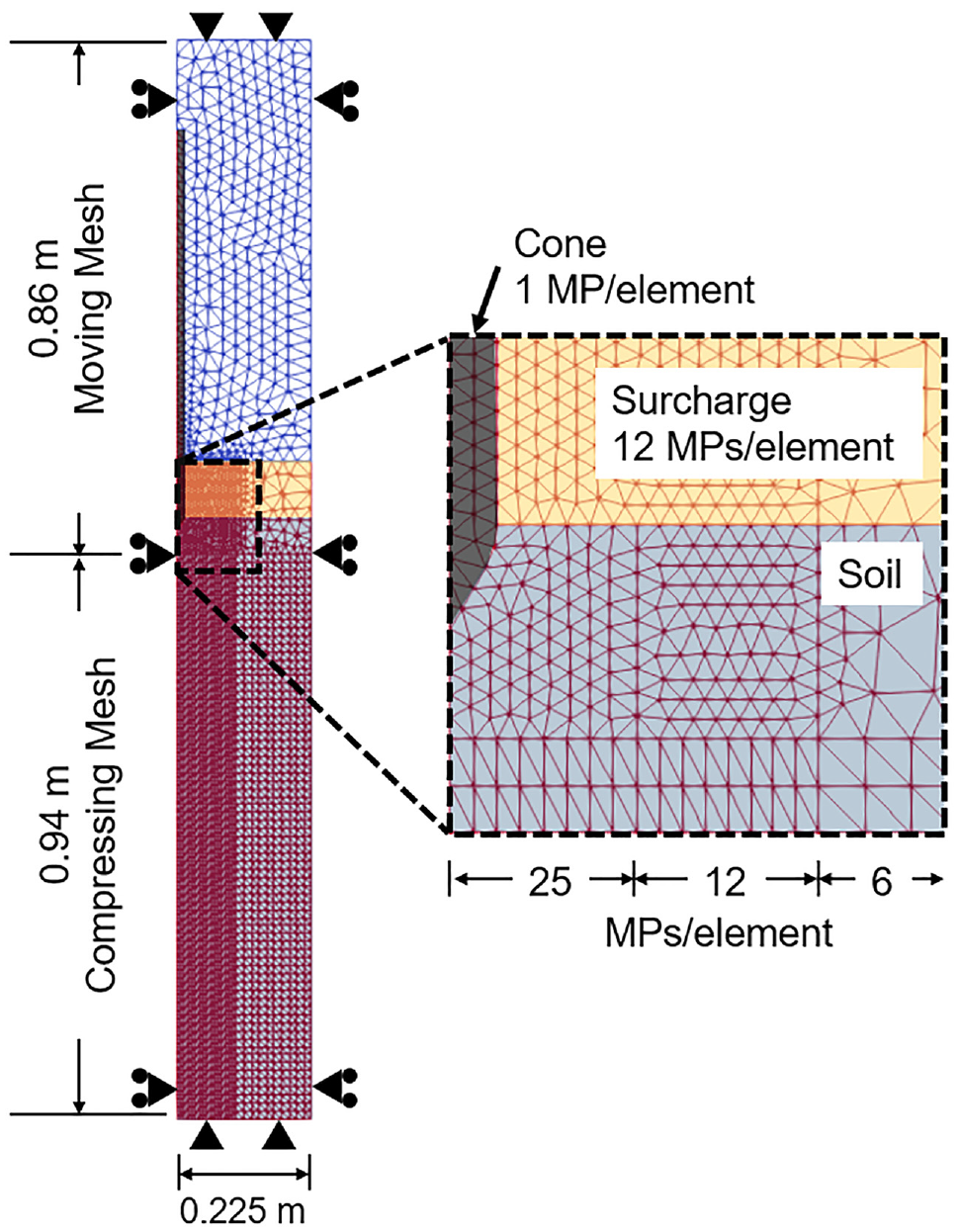
Geometry and discretization of material point method model.

A triangular mesh with a more refined region near the zone of penetration was used. The mesh extended vertically ∼1 m below the tip of the cone and horizontally ∼0.225 m. The radial dimension is slightly smaller than what was used in the laboratory experiments, but for these particular simulations, the radial dimension was shown to play a relatively small role in tip resistance sensitivity in layered zones (Yost et al., 2023). Material points (MPs), that is, numerical integration points in MPM, were more concentrated in the zone of penetration. The moving mesh extended from the top of the domain to ∼0.06 m below the tip of the cone. The compressing mesh began where the moving mesh ended and extended to the bottom boundary. The left and right boundaries were fixed in the horizontal direction, and the top and bottom boundaries were fixed in the horizontal and vertical directions. The boundary conditions replicate the conditions in the laboratory calibration chamber, namely a rigid radial boundary.

Overview of MPM simulations

To generate the numerical portion of this database, 15 highly interlayered soil profiles were created. Each profile consisted of a 0.1-m-thick sand layer overlying a 0.4-m-thick zone of alternating clay and sand layers overlying a 0.5-m-thick sand layer. The stratigraphy of the layered zone was created by randomly selecting a number of layers (up to 40) and randomly selecting layer thicknesses from an exponential distribution with a minimum layer thickness of 0.01 m (0.4d_cone) and mean layer thickness of 0.03 m (1.2d_cone). The geometry of each profile is shown in Figure 7.

Figure 7.

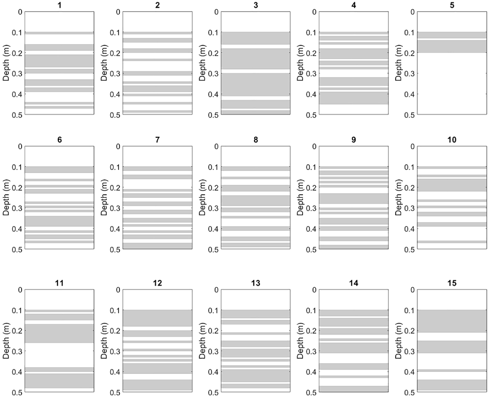
Fifteen soil profiles generated for material point method simulations. Gray zones represent clay layers, and white zones represent sand layers. Note that soil profiles extend to ∼1 m, but only the interlayered zones are shown in this figure.

In total, 30 MPM CPT simulations were performed, resulting from two iterations on each of the 15 soil profiles shown in Figure 7. The first 15 simulations assumed the sand layers were medium dense (D_R = 54%), and the second 15 assumed the sand layers were loose (D_R = 36%). The clay properties were assumed to be the same for both sets of simulations. Constitutive property selection was guided by the results from triaxial tests and finalized by calibrating the MPM model outputs with the analogue laboratory calibration chamber tests. The constitutive parameters are summarized in Table 5. The sand behavior was represented as completely drained using a strain-softening Mohr–Coulomb (SSMC) model. The SSMC model was selected based on observed strain-softening behavior of Baskarp sand in triaxial tests performed by Ibsen and Bødker (1994) and Borup and Hedegaard (1995). The constitutive parameters used in the SSMC model are peak and residual effective friction angles (ϕ’_p and ϕ’_r), peak dilatancy angle (ψ), Young’s Modulus (E), and shape factor (η), which is a parameter that describes the rate of decreasing shear strength with increasing deviatoric strain (Yerro, 2015). The clay behavior was represented as completely undrained using the Tresca model. The undrained shear strength, s_u, was calibrated with undrained anisotropically consolidated triaxial tests conducted by De Lange (2018). Detailed calibration procedures for the sand and clay parameters are provided in the work by Yost et al. (2022b) and are not further elaborated on here.

Table 5.

Constitutive parameters for sand and clay layers in MPM models

Sand layers	Sand relative density, D_r (%)	36	54
	Porosity, n	0.435	0.415
	Peak friction angle, ϕ’_p (°)	37	38
	Residual friction angle, ϕ’_r (°)	35.5	36
	Peak dilatancy angle, ψ (°)	9.5	12
	Young’s Modulus, E (kPa)	10,000	20,000
	Shape factor, η	5	5
	Interface friction coefficient	0.335	0.344
	Poisson ratio, ν	0.33	0.33
Clay layers	Young’s Modulus, E_u (kPa)	25,000	25,000
	Undrained shear strength, s_u (kPa)	27	27
	Poisson ratio, ν_u	0.49	0.49
	Porosity, n	0.3458	0.3458
	Interface friction coefficient	0.335	0.344

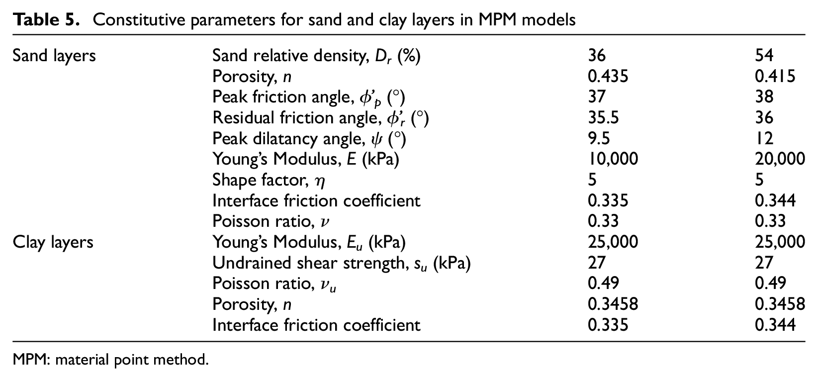
MPM: material point method.

The interface friction coefficient for the sand–cone interface was assumed to be tan(0.5ϕ’_p). The interface friction coefficient of the clay was selected to be equal to the interface friction coefficient of the sand used in the analysis. In this implementation of Anura3D, it is not possible to define average contact properties for elements containing both sand and clay MPs. A sensitivity analysis performed by Yost et al. (2022b) supported using the contact properties associated with the sand to represent contact throughout the layered zones, where the elements immediately adjacent to the cone contain both sand and clay MPs.

Determining tip resistance from MPM simulations

The tip resistance profiles obtained from each of the 30 MPM CPT simulations in the layered soil profiles shown in Figure 7 are taken as q^m. The true tip resistances associated with the sand and the clay layers (q^t_sand and q^t_clay) were determined from three supplemental simulations performed in homogeneous sand (at D_R = 36% and D_R = 54%) and clay profiles using the constitutive properties provided in Table 5. Based on the D_R of the sand in the layered profiles, each q^m was then grouped with an appropriate q^t_sand and q^t_clay.

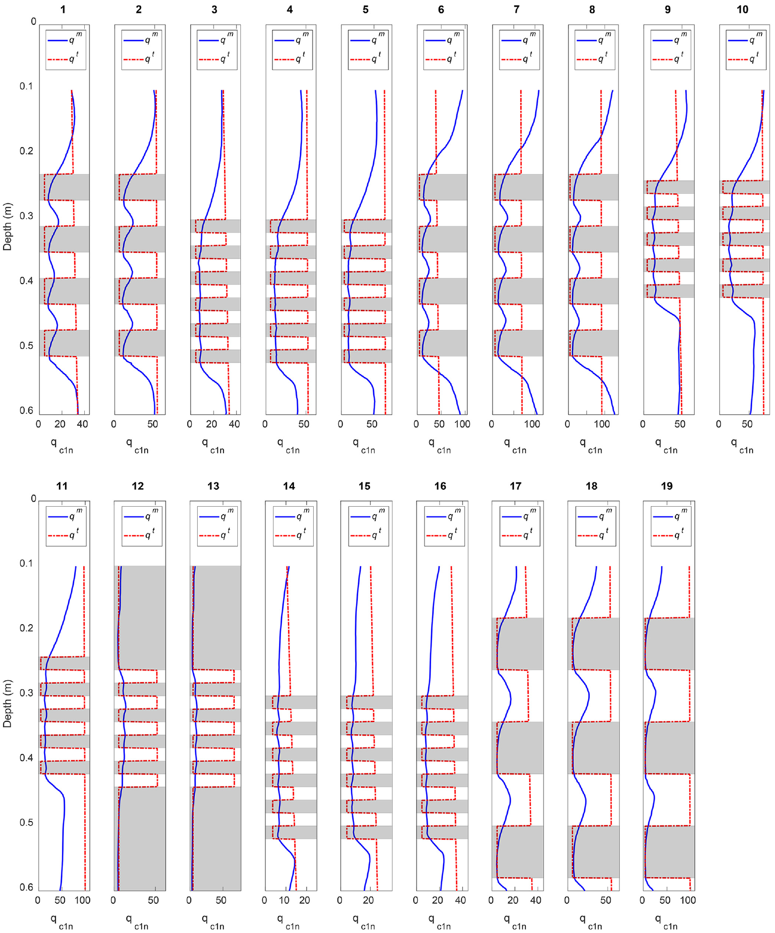
The q^m, q^t_sand, and q^t_clay profiles were truncated between 0.1005 and 0.5005 m—the interlayered zone—and smoothed (averaged) over 0.001 m increments. The smoothing is required because the MPM simulations produce tip resistance values at very small-scale, inconsistent depth increments. The 0.001 m increments were chosen to match the depth interval used in the laboratory data. All tip resistances were then normalized to q_c1n values per the procedure described previously. Finally, coupled with the known layer geometries shown in Figure 7, the q^t profiles were constructed by assigning either q^t_sand or q^t_clay over the depths associated with the sand and clay layers, respectively. The resulting q^m and q^t pairs are shown in Figure 8.

Figure 8.

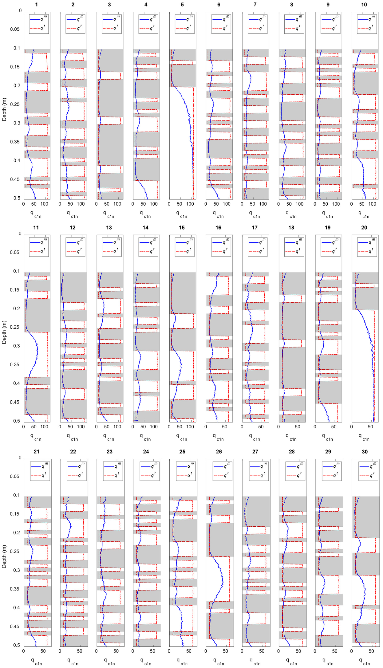
Pairs of q^m and q^t generated from MPM simulations—CPTs 1 through 30. Clay layers are indicated in gray; sand layers are indicated in white. MPM database CPT number is shown above each plot. MPM: material point method; CPT: cone penetration test.

Compilation and structure of database

The laboratory data and MPM data were compiled into two *.csv files, one containing q^m data and one containing q^t data. The first row of each *.csv file contains the depths at which the data were sampled (i.e. 0.1005 m to 0.6005 m at 0.001 m increments). Both laboratory and MPM data were sampled at the same depth increments, but the total depth of the laboratory profiles was larger. Therefore, the MPM data were padded with zeros on the end to match the depth dimension of the laboratory data. Each subsequent row represents one CPT. Rows 2 through 20 contain the tip resistances from each of the 19 laboratory CPTs. Rows 21 through 50 contain the tip resistances from each of the 30 MPM CPTs.

The first column of each *.csv file contains a “profile category” number. Profiles that had the same layer geometry were grouped together. For example, laboratory CPTs 3 through 5 were assigned the same profile category number. Similarly, MPM CPTs 1 and 16 were assigned the same profile category number. The intent of grouping similar profiles is to improve potential statistical learning applications for this data set. When training statistical learning algorithms, data are parsed into training and test data sets. By assigning the same profile category number to similar profiles, it is possible to ensure that all profiles that fall within that category are assigned to either the training or test data set, and not split between the two. This avoids potential problems with the statistical learning algorithm, which could potentially “memorize” a pattern already seen in the training data and apply it to a similar profile in the test data, without truly learning the relationship between q^m and q^t.

How to access, supplement, and use the database

The database is available on the Virginia Tech data repository, VTechData (Yost et al., 2022c). Two *.csv files are provided, one containing q^m data and one containing q^t data, as described in the previous section. A Jupyter notebook (created in the Google Colab environment) is also provided at the same location to read the data and perform initial processing. Contents of the notebook include the following:

A script to read data in and initialize depth, q^m, q^t, and profile category variables;

A script to visualize the contents of the database;

A framework to parse the database into separate training and test data sets, grouping profiles with the same profile category number together;

A script to visualize the parsed training and testing data;

An example of how to manipulate data with subsampling and filtering to change the size of the depth interval;

An example of “chunking” profiles to generate more data to use in training and testing data sets;

A framework for how to add data to the existing database;

An example of using a profile from the database to assess a simple blurring filter.

Example uses

Two potential uses of this database to develop better multiple thin-layer correction procedures are (1) to assess existing blurring filters and develop better ones through statistical learning methods and (2) to directly assess the performance of procedures (i.e. assess how well q^inv or q^corr matches q^t). Those applications are demonstrated in the following two sections.

Assessing a CPT blurring filter

The selection of a filter that adequately captures the blurring effect of the CPT passing through interlayered soil is critical to the success of inverse-style multiple thin-layer correction procedures. The Jupyter notebook provides an example of how to visually assess the performance of such a filter on q^m and q^t data from a single profile. A simple triangular distribution and a chi-squared distribution are provided as filter options. Any other filter could easily be implemented into the notebook by the user. The convolution of the filter (e.g. the chi-squared filter shown in Figure 9a) with q^t generates a q^m,sim that can be compared with q^m (e.g. Figure 9b). As shown in Figure 9b, since the mismatch between q^m and q^m,sim is large, the chosen filter (Figure 9a) is not a good representation of the physics of multiple thin-layer effects.

Figure 9.

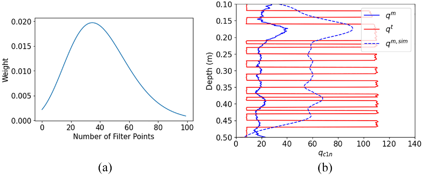
(a) Chi-squared blurring filter and (b) comparison of q^m, q^t, and q^m,sim generated by convolving the chi-squared blurring filter shown in (a) with q^t.

This database has been structured to support the development of better-blurring filters using statistical learning tools. For example, a neural network could be trained to predict q^m given q^t using the parsed training and test data provided in the database. Once trained, the neural network could be inserted within the framework of an existing inverse-style multiple thin-layer correction procedure (like Cooper et al., 2022) to describe the blurring process.

Assessing efficacy of multiple thin-layer correction procedures

The database can also be used to directly assess the efficacy of multiple thin-layer correction procedures. Using q^m as the input to the procedure, the output (q^corr or q^inv) is computed and compared directly to q^t. For example, in Figure 10, the performance of the following multiple thin-layer correction procedures is compared: Boulanger and DeJong (2018) inverse procedure (BD18), Cooper et al. (2022) inverse procedure (Cea22), and Yost et al. (2021) forward “Deltares” procedure (DEL21).

Figure 10.

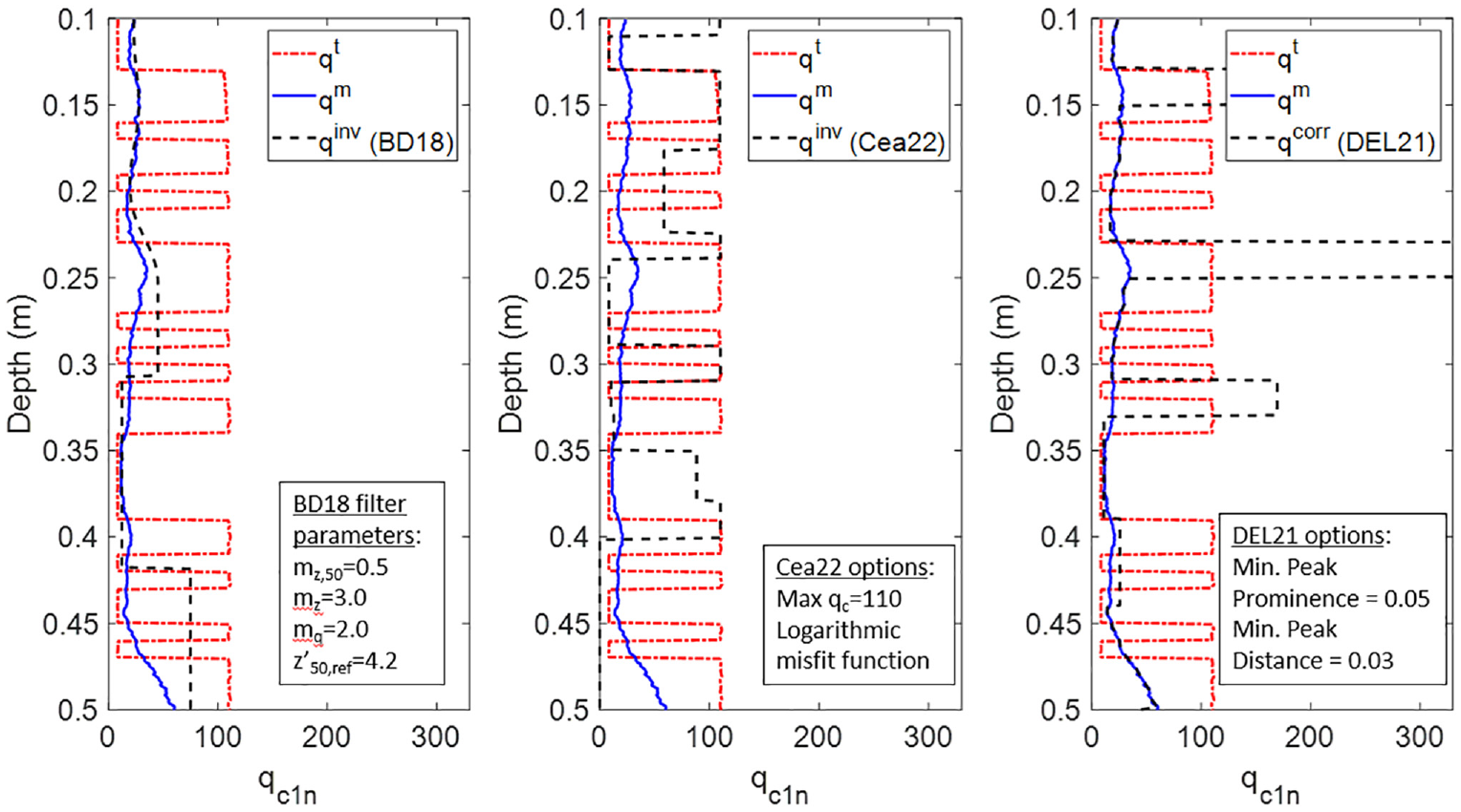
Efficacy of multiple thin-layer correction procedures on MPM Database CPT Number 6 from this database: (a) Boulanger and DeJong (2018) (BD18), (b) Cooper et al. (2022) (Cea22), and (c) Yost et al. (2021)“Deltares” (DEL21).

None of the procedures shown in Figure 10 perform well—none yield q^corr or q^inv values that are good estimates of q^t. This is not surprising and has been shown in previous studies for other soil profiles with layer thicknesses on the order of 1.6d_cone or thinner (e.g. Yost et al., 2021). This highlights the need to improve these procedures or to develop new techniques to estimate q^t from q^m. This database has been structured to aid in the development of new multiple thin-layer correction procedures, using statistical learning tools in particular. For example, a small neural network could possibly be developed using the parsed training and test data provided in this data set to attempt to predict q^t for a given q^m. A potential pitfall of this is that the neural network would serve as a black box method to extract q^m. In other words, no greater understanding of the physics of multiple thin-layer effects would be achieved, there is little control of what q^m could potentially look like, and it may be difficult to implement known physical constraints. Furthermore, the performance of the procedure would have to be carefully evaluated if used on profiles that were very different from the profiles used to train and test the procedure.

Nuances and limitations

The use of any database comes with limitations. This section discusses some of the relevant nuances and limitations of this database.

Limitations of the numerical model

It is important to acknowledge that any numerical technique has inherent limitations on how well it can represent soil behavior. MPM is a continuum method, meaning micro-scale phenomena like particle crushing and breakage are not directly accounted for. At the high mean effective stresses experienced by the soil during cone penetration, particle breakage is possible. Furthermore, simple soil constitutive models were used for the simulations in this article; more advanced constitutive models may be useful in better-describing soil behavior over large ranges of stresses. However, the use of more advanced constitutive models also introduces more uncertainties and may not produce better results (e.g. as discussed by Yost et al., 2023).

Many assumptions and simplifications are made when developing a numerical model to replicate a real-world scenario with respect to the geometry, boundary conditions, drainage conditions, soil properties, soil–cone contact properties, and other parameters (Yost et al., 2023). The MPM simulations used to generate the numerically simulated data in this database have been extensively calibrated with laboratory data. In that sense, some of the uncertainties associated with those assumptions have been reduced, and the MPM results presented in this article can be considered a direct extension of the laboratory results in which new geometries have been introduced. However, the profile geometries used for the MPM simulations have not been replicated with laboratory testing. It would be useful to perform additional laboratory CPT testing with irregular soil layering and layers as thin as 0.4d_cone, like the profiles used for the MPM simulations, to further validate the MPM results. Another way to indirectly assess the validity of the MPM data could be to use laboratory data only to train a multiple thin-layer correction procedure, and then test it on the MPM data (or vice versa).

Sensitivity to CPT sampling interval

Typical CPTs record data at 10 mm to 50 mm depth intervals. The depth interval for both the laboratory and MPM data in this database is 1 mm. When using this database, there may be a desire to more coarsely sample (subsample) the data to better represent typical CPT sampling intervals. Two example techniques on how to do this include standard subsampling (i.e. selecting data at a regular depth interval) and subsampling with interpolation (i.e. linearly interpolating the data to the depth interval the user chooses). An example of each technique is included in the Jupyter notebook provided as supplemental material to this article. However, there are potential pitfalls of more coarsely sampling the data. While coarser sampling better represents how a typical CPT records q^m, it may not result in a good representation of q^t. For example, sampling at a 20 mm interval may result in zero or one data points in a 10-mm-thick layer (the minimum layer thickness used in these profiles). This could prove to be problematic when using the more coarsely sampled data to develop or train multiple thin-layer correction procedures because it will not accurately preserve the piecewise nature of q^t. Therefore, for this database, we recommend that q^t be sampled at no finer than one half the minimum layer thickness in the profiles (i.e. 5 mm). Offsetting the sampling interval to avoid data points falling on the transition zone between layers is also recommended and will improve resolution of q^t by ensuring two data points fall within each layer. This approach is demonstrated in Figure 11. If a coarser sampling interval is desired, we suggest that q^m is sampled at that coarser interval, and then resampled at no finer than one half the minimum layer thickness in the profiles, matching our recommendation for subsampling q^t. This will reduce resolution in q^m (but may be more representative of field conditions) and preserve the required resolution in q^t.

Figure 11.

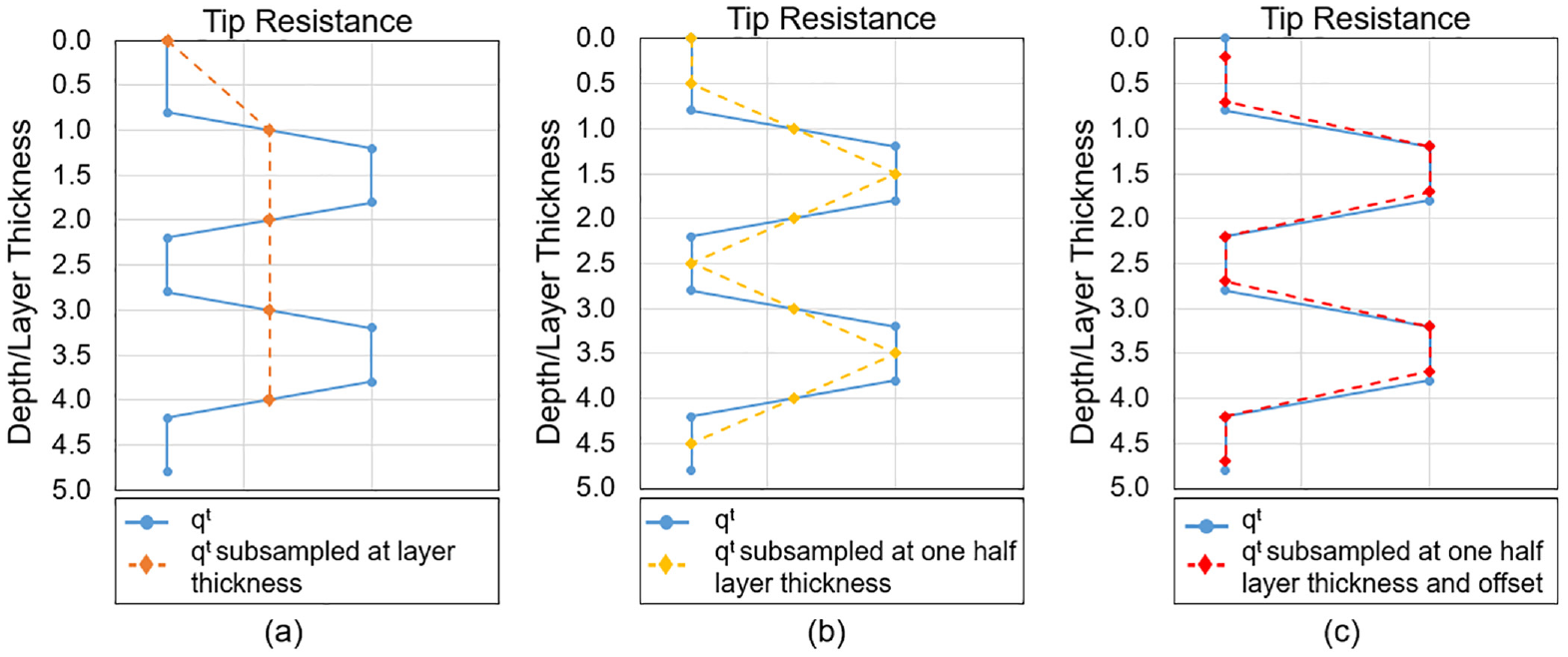
Sensitivity of q^t to subsampling interval. For a normalized layer thickness equal to unity, subsampling with a depth interval (a) equal to the layer thickness, (b) equal to one half the layer thickness, and (c) equal to one half the layer thickness, but offset such that two data points are captured in each layer and no data point falls on the layer boundary.

It is also important to consider the impact of sampling interval when extending the procedures developed using this database to field data. In coarsely sampled field data (q^m), soil layers with thicknesses less than the sampling interval may be “hidden” in the sense that there is no data point recorded directly in the layer. However, the influence of those hidden layers may still be captured by adjacent data points due to multiple thin-layer effects. Yost et al. (2022b) showed that a 0.4d_cone-thick, soft clay layer embedded in a stiffer sand layer could be easily identified in numerically generated CPT data. Even if the data were sampled at a 50 mm depth interval, the thin-layer effect was still captured. Therefore, it is reasonable to attempt to extract a q^t that includes layers thinner than the sampling interval (though it may be more difficult). Note that Yost et al. (2022b) showed that in a profile with multiple, alternating 0.4d_cone-thick layers of stiffer sand and softer clay, variation in q^m in the layered zone was completely obscured. To extract the correct q^t for such a profile, an inverse multiple thin-layer correction procedure that does not rely exclusively on variation in q^m to make its “guess” of q^t (e.g. the Cooper et al., 2022 procedure) is required.

In general, we recommend the smallest practical sampling interval when performing a CPT in highly interlayered stratum. To obtain q^t from the field q^m, a multiple thin-layer correction procedure must be applied. When applying these procedures to field data, we suggest that first, q^m be more finely interpolated at a depth interval equal to one half the thickness of the finest layer you are trying to identify in q^t. This approach helps bridge the gap between procedures developed using the finely sampled data in this database and more coarsely sampled field data. Research using this database should include sensitivity analyses considering different sampling techniques and intervals to achieve optimum results.

Limitations of statistical learning applications with this database

Statistical learning techniques require training data. While data augmentation techniques may be used (such as the data chunking method presented as an example in the Jupyter notebook), the database presented herein is likely too small to robustly train, for example, a high-dimensional neural network. Each soil profile contained in this database is less than 0.6 m deep: a function of limited laboratory calibration chamber depths and the computational cost of numerically simulating CPTs. This inherently limits the amount of data within a single CPT profile. Furthermore, this database only contains 49 soil profiles. The addition of more data would be largely beneficial for the potential statistical learning applications of this database.

The more variety in the training and testing data, the better, because there would be less extrapolation to unseen conditions. That means the addition of q^m and q^t data with varied profile geometries and soil properties would be better than performing additional simulations with the 15 geometries used to generate the existing database. Furthermore, the existing database contains only bimodal q^t data: in other words, the profiles contain only two soil types (sand and clay) each with one set of material properties. Ideally, additional simulations would be performed in profiles generated with randomly assigned geometries, material types, and material properties for each layer. This would result in more irregular q^t distributions that may better mimic real-world conditions. Furthermore, it would help validate correction procedures for additional soil types. Currently, the Anura3D platform used to generate the database requires the manual generation of profile geometries in the GiD (2020) preprocessor. The profile geometry generation process would need to be automated to realistically facilitate large-scale testing of more randomly generated profiles.

Conclusions and future research directions

In this article, a CPT database developed from laboratory and numerically simulated data was presented. Measured and true tip resistance (q^m and q^t) pairs for 49 different highly interlayered soil profiles were generated and compiled into a publicly available data set. A companion Jupyter notebook is provided to facilitate the use of these data; in particular, to train statistical learning techniques to either predict q^t from q^m, or to develop a better-blurring model of how the CPT translates q^t to q^m through the phenomenon referred to as multiple thin-layer effects. Examples of how to use this database to assess existing blurring models and multiple thin-layer correction procedures were provided. Several nuances and limitations of the database were discussed, and the need for more data was highlighted. Future work from the authors aims to contribute more data to the database within the framework presented in this article from the results of new laboratory calibration chamber studies being performed at Virginia Tech. In addition, the authors intend to use the database to improve the blurring model used in the Cooper et al. (2022) multiple thin-layer correction procedure. Contributions to the database from other researchers are encouraged to develop a more robust set of open data needed for statistical learning techniques and to help standardize the way the efficacy of multiple thin-layer correction procedures is assessed.

Footnotes

Acknowledgements

Review comments from Dr. Adrian Rodriguez-Marek were greatly appreciated. Conversations with Dirk de Lange also shed light on important topics.

Declaration of Conflicting Interests

The author(s) declared no potential conflicts of interest with respect to the research, authorship, and/or publication of this article.

Funding

The author(s) disclosed receipt of the following financial support for the research, authorship, and/or publication of this article: This research was partially funded by NSF (grant nos. CMMI-1825189 and CMMI-1937984). However, any opinions, findings, conclusions, or recommendations expressed in this material are those of the authors and do not necessarily reflect the views of National Science Foundation (NSF) or others acknowledged.

ORCID iD

Kaleigh M Yost

References

Ahmadi

Robertson

(2005) Thin-layer effects on the CPT qc measurement. Canadian Geotechnical Journal 42(5): 1302–1317.

Al-Kafaji

IKJ

(2013) Formulation of a dynamic material point method (MPM) for geomechanical problems. PhD Thesis, University of Stuttgart, Stuttgart.

Anura3D (2021) Anura3D MPM Research Community. Available at: http://www.anura3d.com/ (accessed 3 May 2021).

Bardenhagen

Guilkey

Roessig

Brackbill

Witzel

Foster

(2001) An improved contact algorithm for the material point method and application to stress propagation in granular material. Computer Modeling in Engineering and Sciences 2(4): 509–522.

Baziw

Verbeek

(2022) Methodology for obtaining true cone bearing estimates from blurred and noisy measurements. In: Cone penetration testing 2022 (ed Gottardi Tonni ), Bologna, 8–10 June, pp. 115–120. London: Taylor & Francis Group.

Beuth

(2012) Formulation and application of a quasi-static material point method. PhD Thesis, University of Stuttgart, Stuttgart.

Beuth

Vermeer

(2013) Large deformation analysis of cone penetration testing in undrained clay. In: Installation effects in geotechnical engineering (ed Hicks

Dijkstra

Lloret-Cabot

Karstunen

), Rotterdam, 24–27 March. London: Taylor & Francis Group.

Bisht

Salgado

Prezzi

(2021a) Analysis of cone penetration using the material point method. In: Barla

Di Donna

Sterpi

(eds) Challenges and Innovations in Geomechanics. Cham: Springer, pp. 765–771.

Bisht

Salgado

Prezzi

(2021b) Material point method for cone penetration in clays. Journal of Geotechnical and Geoenvironmental Engineering 147(12): 1–16.

10.

Borup

Hedegaard

(1995) Baskarp sand no. 15. Data report 9403, January. Aalborg: Geotechnical Engineering Group.

11.

Boulanger

DeJong

(2018) Inverse filtering procedure to correct cone penetration data for thin-layer and transition effects. In: Cone penetration testing 2018 (ed Hicks Pisano Peuchen ), Delft, 21–22 June, pp. 25–44. London: Taylor and Francis Group.

12.

Boulanger

Moug

Munter

Price

Dejong

(2016) Evaluating liquefaction and lateral spreading in interbedded sand, silt, and clay deposits using the cone penetrometer. In: 5th international conference on geotechnical and geophysical site characterisation (ISC’5), Gold Coast, QLD, Australia, 5–9 September, pp. 81–97. The Gap, QLD, Australia: Australian Geomechanics Society.

13.

Ceccato

Simonini

(2017) Numerical study of partially drained penetration and pore pressure dissipation in piezocone test. Acta Geotechnica 12: 195–209.

14.

Ceccato

Simonini

(2019) Numerical features used in simulations. In: Fern

Rohe

Soga

Alonso

(eds) The Material Point Method for Geotechnical Engineering. Boca Raton, FL: Taylor & Francis Group, pp. 101–124.

15.

Ceccato

Beuth

Simonini

(2015) Study of the effect of drainage conditions on cone penetration with the material point method. In: XV Pan-American conference on soil mechanics and geotechnical engineering, Buenos Aires, Argentina, 15–19 November.

16.

Ceccato

Beuth

Simonini

(2016a) Analysis of piezocone penetration under different drainage conditions with the two-phase material point method. Journal of Geotechnical and Geoenvironmental Engineering 142(12): 04016066.

17.

Ceccato

Beuth

Vermeer

Simonini

(2016b) Two-phase material point method applied to the study of cone penetration. Computers and Geotechnics 80: 440–452.

18.

Cooper

Martin

Yost

Yerro

Green

(2022) Robust identification and characterization of thin soil layers in cone penetration data by piecewise layer optimization. Computers and Geotechnics 141: 104404.

19.

Cox

McLaughlin

Van Ballegooy

Cubrinovski

Boulanger

Wotherspoon

(2017) In-situ investigation of false-positive liquefaction sites in Christchurch, New Zealand: St. Teresa’s School Case History. In: Performance-based design in earthquake geotechnical engineering (PBD-III) (ed M

Taiebat

), Vancouver, BC, Canada, 16–19 July.

20.

de Greef

Lengkeek

(2018) Transition-and thin layer corrections for CPT based liquefaction analysis. In: Cone penetration testing 2018 (ed Hicks Pisano Peuchen ), Delft, 21–22 June, pp. 317–322. London: Taylor & Francis Group.

21.

De Lange

(2018) CPT in thinly layered soils. Report, NAM, August.

22.

Ghasemi

Calvello

Martinelli

Galavi

Cuomo

(2018) MPM simulation of CPT and model calibration by inverse analysis. In: Cone penetration testing 2018 (ed Hicks Pisano Peuchen ), Delft, 21–22 June, pp. 295–301. London: Taylor & Francis Group.

23.

GiD (2020) The personal pre and post processor Barcelona (Spain): CIMNE. Available at: www.gidsimulation.com (accessed 28 February 2023).

24.

Hudson

Ulmer

Zimmaro

Kramer

Stewart

Brandenberg

(2023) Unsupervised machine learning for detecting soil layer boundaries from cone penetration test data. Earthquake Engineering and Structural Dynamics 52: 3201–3215.

25.

Ibsen

Bødker

(1994) Baskarp sand no.15. Data report 9301, August. Aalborg: Geotechnical Engineering Group.

26.

Idriss

Boulanger

(2008) Soil Liquefaction during Earthquakes (Monograph MNO-12). Oakland, CA: Earthquake Engineering Research Institute.

27.

Khosravi

DeJong

Boulanger

Khosravi

Hajialilue-Bonab

Sinha

Wilson

(2022) Centrifuge tests of cone-penetration test of layered soil. Journal of Geotechnical and Geoenvironmental Engineering 148(4): 04022002.

28.

McLaughlin

(2017) Investigation of false-positive liquefaction case histories in Christchurch, New Zealand. MS Thesis, The University of Texas at Austin, Austin, TX.

29.

Martinelli

Galavi

(2021) Investigation of the material point method in the simulation of cone penetration tests in dry sand. Computers and Geotechnics 130: 103923.

30.

Martinelli

Galavi

(2022) An explicit coupled MPM formulation to simulate penetration problems in soils using quadrilateral elements. Computers and Geotechnics 145: 104697.

31.

Maurer

Green

Cubrinovski

Bradley

(2014) Evaluation of the liquefaction potential index for assessing liquefaction hazard in Christchurch, New Zealand. Journal of Geotechnical and Geoenvironmental Engineering 140(7): 04014032.

32.

Molina-Gómez

Cordeiro

Ferreira

Viana da Fonseca

(2022) Soil stratigraphy from seismic piezocone data and multivariate clustering in alluvial soil deposits: Experience in the Lower Tagus Valley region. In: Cone penetration testing 2022 (ed Gottardi Tonni ), Bologna, 8–10 June, pp. 584–590. London: Taylor & Francis Group.

33.

Schmertmann

(1978) Guidelines for cone penetration test performance and design. Report, US Department of Transportation Federal Highway Administration, Washington, DC, July.

34.

Sulsky

Chen

Schreyer

(1994) A particle method for history-dependent materials. Computer Methods in Applied Mechanics and Engineering 118(1–2): 179–196.

35.

Tehrani

Galavi

(2018) Comparison of cavity expansion and material point method for simulation of cone penetration in sand. In: Cone penetration testing 2018 (ed Hicks Pisano Peuchen ), Delft, 21–22 June, pp. 611–615. London: Taylor & Francis Group.

36.

Yerro

(2015) MPM modelling of landslides in brittle and unsaturated soils. PhD Thesis, Universitat Politecnica de Catalunya, Barcelona.

37.

Yost

Cooper

Green

Martin

Yerro

(2022a) Correcting measured CPT tip resistance for multiple thin-layer effects. In: Cone penetration testing 2022 (ed Gottardi Tonni ), Bologna, 8–10 June 2022, pp. 778–783. London: Taylor & Francis Group.

38.

Yost

Cox

Wotherspoon

Boulanger

Van Ballegooy

Cubrinovski

(2019) In situ investigation of false-positive liquefaction sites in Christchurch, New Zealand: Palinurus Road case history. Geotechnical Special Publication 308: 436–451.

39.

Yost

Green

Upadhyaya

Maurer

Yerro-Colom

Martin

Cooper

(2021) Assessment of the efficacies of correction procedures for multiple thin layer effects on cone penetration tests. Soil Dynamics and Earthquake Engineering 144: 106677.

40.

Yost

Martinelli

Yerro

Green

de Lange

(2023) Addressing complexities in MPM modeling of cone penetrometer tests in homogenous and highly interlayered soils. Computers and Geotechnics 158(2023): 105378.

41.

Yost

Yerro

Green

Martin

Cooper

(2022b) MPM modeling of cone penetrometer testing for multiple thin-layer effects in complex soil stratigraphy. Journal of Geotechnical and Geoenvironmental Engineering 148(2): 04021189.

42.

Yost

Yerro Colom

Martin

Green

(2022c) Data associated with A CPT database for multiple thin-layer correction procedure development [Dataset]. University Libraries, Virginia Tech. https://doi.org/10.7294/21408450

43.

Zambrano-Cruzatty

Yerro

(2020) Numerical simulation of a free fall penetrometer deployment using the material point method. Soils and Foundations 60(3): 668–682.

A cone penetration test database for multiple thin-layer correction procedure development

Abstract

Keywords

Introduction

Development of CPT database

Laboratory data

Overview

Determining tip resistance from overburden pressure and density for sands

Determining tip resistance from overburden pressure and undrained shear strength for clays

Normalizing the laboratory data

Constructing measured and true tip resistance profiles

Assessing efficacy of empirical relationships and uncertainties in laboratory data

Numerically simulated data

MPM background

Overview of MPM simulations

Determining tip resistance from MPM simulations

Compilation and structure of database

How to access, supplement, and use the database

Example uses

Assessing a CPT blurring filter

Assessing efficacy of multiple thin-layer correction procedures

Nuances and limitations

Limitations of the numerical model

Sensitivity to CPT sampling interval

Limitations of statistical learning applications with this database

Conclusions and future research directions

Footnotes

Acknowledgements

Declaration of Conflicting Interests

Funding

ORCID iD

References