
Abstract
With the improvement of the world’s largest seafloor observation network (S-net) and the increase in the quantity and quality of records, the ergodic assumptions can be further relaxed in the modeling of offshore ground motion models (GMMs). This allows accounting for systematic and repeatable source, site, and path effects to further understand the characteristics of offshore ground motion in the Japan Trench region. We developed an offshore ergodic backbone GMM for subduction earthquakes and classified the sites into four categories using horizontal–vertical response spectral ratio to investigate site amplification. The offshore ergodic GMM is applicable for subduction earthquake scenarios with moment magnitudes ranging from 4.0 to 7.4 and rupture distances ranging from 10 to 300 km. Comparing offshore ergodic GMMs with onshore GMMs for subduction earthquakes, we found that offshore GMMs were significantly different from onshore GMMs, especially in the long-period and unburied states. Then a new offshore non-ergodic GMM was developed based on the offshore ergodic GMM. The systematic and repeatable source and site effects were captured by the spatially varying coefficients represented by Gaussian processes, while the systematic and repeatable path effects were captured by cell-specific anelastic attenuation proposed by Dawood and Rodriguez-Marek (2013), calculated with the Cohen-Sutherland computer graphics algorithm. The non-ergodic GMM revealed systematic and repeatable source, site, and path effects that were not captured by the ergodic GMM. Moreover, the non-ergodic GMM showed reduced aleatory variability and epistemic uncertainty on ground motion estimation compared to ergodic GMM. The reduction of aleatory variability and epistemic uncertainty had a significant impact on probabilistic seismic hazard analysis. Quantifications of these results are contributed to conduct reasonable seismic design and seismic risk assessment for marine engineering in offshore regions vulnerable to strong subduction earthquakes.
Keywords
Introduction
The current research indicates that the offshore ground motion is significantly different from the onshore ground motion in response spectrum (Chen et al., 2015; Dhakal et al., 2021; Hu et al., 2020; Zhang and Zheng, 2019), temporal characteristics (Zhang and Zheng, 2020), elastic relative and absolute input energy (Hu and Tan, 2022), vertical-to-horizontal spectrum ratio (Boore and Smith, 1999; Chen et al., 2017; Tan and Hu, 2021), damping modification factors (Hu et al., 2022b), and seismic ground motion simulation (Lan et al., 2021; Li et al., 2011), especially for subduction earthquakes. Furthermore, Tan and Hu (2023) compared the differences in horizontal peak ground acceleration (PGA), spectral acceleration, frequency content, and significant duration between offshore and onshore ground motion characteristics using two large offshore earthquakes (February 13, 2021, Mw 7.1 and March 17, 2022, Mw 7.4), wherein the offshore records were from the S-net network and the onshore records were from the K-NET network. Cui et al. (2023) employed the same method to analyze offshore and onshore ground motion characteristics for a large earthquake. Both studies revealed significant differences and factors influencing the characteristics of offshore and onshore ground motion.
Strong offshore ground motion could cause the destruction of structures (Li et al., 2022), such as the collapse and damage of cross-sea bridges and submarine tunnels (Zhang et al., 2016), the leaking of marine oil drilling platforms (Borrero, 2005), the fracturing of submarine communication cables (Bi and Hao, 2016), and the large-scale liquefaction of artificial island backfills (Tanaka, 2000). For example, several earthquakes, such as the 2011 Mw 9.0 Tohoku-Oki subduction interface earthquake (Simons et al., 2011) and the 2021 Mw 7.1 Fukushima subduction intraslab earthquake (Kiser and Kehoe, 2021; Kubota et al., 2021), have revealed substantial economic losses and secondary disasters (e.g. tsunami, mudslide, etc.) caused by ground motions in Japan trench area. Therefore, with the development of performance-based earthquake engineering, it is necessary to conduct reasonable seismic design and seismic risk assessment of marine engineering in offshore regions that are easily affected by strong subduction earthquakes, such as the east and south coasts of China, Chile, the west coast of the United States, New Zealand, and Japan.
Under the current concept of performance-based seismic engineering, probabilistic seismic hazard analysis (PSHA) is based on empirical ground motion models (GMMs). In PSHA, the slope of the hazard curve is sensitive to aleatory standard deviation (SD) of empirical GMMs (Bommer and Abrahamson, 2007). The ergodic assumption is convenient because it combines ground motion data from similar tectonic environments around the world to develop ergodic GMMs based on magnitude, distance, and site conditions. For partially non-ergodic GMMs, there are two descriptions: one can only capture the systematic site effects, known as single station GMMs; the other is that GMMs have different coefficient values for different regions, such as constant term, anelastic attenuation term, site term, and basin amplification term. Fully non-ergodic GMMs include non-ergodic terms to capture the systematic effects (e.g. source, path, and site). For example, the NGA-west1 (e.g. Abrahamson and Silva, 2008; Boore and Atkinson, 2008; Campbell and Bozorgnia, 2008; Chiou and Youngs, 2008; Idriss, 2008) GMMs are fully ergodic GMMs for shallow crustal tectonic settings. In addition, four of the NGA-west2 (e.g. Abrahamson et. al., 2014; Boore et al., 2014; Campbell and Bozorgnia, 2014; Chiou and Youngs, 2014) GMMs are partially non-ergodic GMMs for shallow crustal tectonic settings because it contains the regional terms in their models. However, there are still regional differences in ergodic GMMs over a wide range of regions, which has led to the development of GMMs for specific regions and non-ergodic GMMs. For instance, many regional ergodic GMMs have already been developed for the Japanese subduction zone (e.g. Si et al., 2020; Zhao et al., 2016a, 2016b; Hassani and Atkinson, 2021). Furthermore, the NGA-Subduction (NGA-Sub) project (Bozorgnia et al., 2022; Mazzoni et al., 2022) established a large subduction ground motion database containing a large number of strong earthquake records from subduction zones around the world and developed new GMMs for subduction earthquakes (e.g. Abrahamson and Gülerce, 2020, 2022; Gregor et al., 2022; Kuehn et al., 2020; Parker et al., 2020, 2022). Note that the NGA-Sub GMMs are also partially non-ergodic GMMs that capture the average differences in ground motion scaling among the seven broad regions by accounting for site term, the linear distance term, basin term, constant term, and break point for large-magnitude scaling. In addition, several recent studies (e.g. Abrahamson et al., 2019; Kuehn, 2021; Kuehn et al., 2019; Landwehr et al., 2016; Lavrentiadis et al., 2021; Lavrentiadis and Abrahamson, 2021; Liu et al., 2022a, 2022b; Macedo and Liu, 2022; Sung et al., 2021) have shown regional differences in the scaling of ground motion represented by the non-ergodic GMMs, revealing systematic and repeatable source, path, and site effects. These studies indicate that the non-ergodic model can capture epistemic uncertainty of spatially varying effects. If the trade-off between the aleatory variability and epistemic uncertainty for seismic risk is insufficient, ergodic GMMs may lead to biased estimates of intensity measures (IMs) hazard curves when performing PSHA (Abrahamson et al., 2019).
With the improvement of the offshore strong-motion network (S-net) and the quantity and quality of subduction earthquake records in the Japan Trench region, the ergodic assumption can be further relaxed in the modeling of offshore GMMs to account for systematic and repeatable source, site, and path effects. In this study, we introduced the S-net seafloor ground motion database and utilized a horizontal-to-vertical response spectral ratio (H/V) with a damping ratio of 5% for each station to classify the site. We then developed the offshore ergodic backbone GMM for subduction earthquakes in the Japan Trench area. Furthermore, we compared our offshore GMM with onshore GMM for subduction earthquakes to gain further insight into offshore ground motion characteristics. We further developed the offshore non-ergodic GMM based on the offshore ergodic backbone GMM. The systematic and repeatable source, site, and path effects of the offshore non-ergodic GMM were modeled using Gaussian processes and cell-specific attenuation approach, respectively. Finally, we discussed the residuals and aleatory SDs of the non-ergodic GMM and the systematic and repeatable source, site, and path effects captured by the non-ergodic GMM, and drew some conclusions. The results of this article are expected to provide a basis for revealing the source, site, and path effects and offshore ground motion characteristics for subduction earthquakes in the Japan Trench region.
S-net seafloor ground motion database
Introduction of S-net seafloor observation network
The S-net is situated in the northeast region of Japan, aligning with the arc boundary where the Pacific plate subducted beneath the Eurasian plate. Its purpose is to enhance the Japan Meteorological Agency’s earthquake early warning (EEW) and tsunami early warning systems (Aoi et al., 2020).
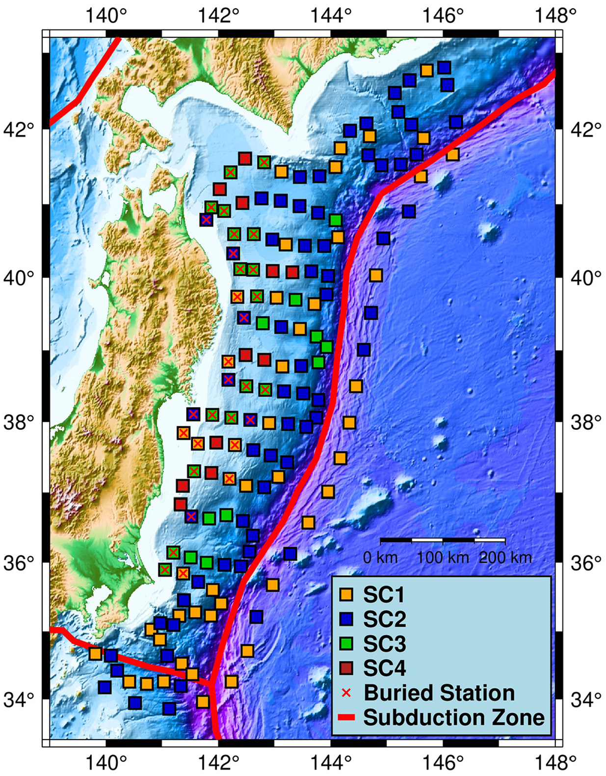
Initiated in 2011 following the catastrophic 9.1 Tohoku-Oki earthquake, the construction of S-net was completed in March 2017. The seafloor observation network consists of six subsystems: S1, S2, S3, S4, S5, and S6. Figure 1 illustrates their geographical distribution. It comprises 150 seafloor observation stations, spanning an area of approximately 1000 km by 300 km from off-Hokkaido to off-Kanto. Stations situated in bathymetry below 1500 m (as shown in Figure 1), numbering 41, are buried in grooves approximately 1 m beneath the seafloor to circumvent fishery activities, minimize ground noise, and enhance ground coupling. The remaining 109 stations are placed freely on the seafloor in areas with bathymetry deeper than 1500 m. These stations are spaced at approximately 30 (50–60) km intervals in the east-west (north-south) direction, perpendicular to (parallel with) the Japan Trench axis. Each subsystem contains 22–28 stations connected in series to land stations via ocean-bottom fiber optic cables, with lengths ranging from 800 to 1500 km. The total length of these cables is approximately 5500 km. The S-net observation device contains built-in sensors, including accelerometers, velocimeters, and pressure gauges. The device has a cylindrical appearance and is placed horizontally along the direction of the cable.
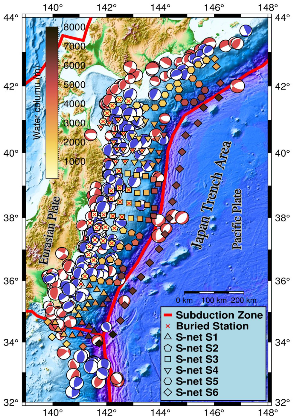
The geographical distribution of the S-net seafloor observation network and earthquake epicenters. The color bar indicates the bathymetry at each observation station. The blue and red hypocentral mechanism symbols represent interface events and intraslab events, respectively. The hypocentral depth of the interface event is smaller than 50 km and that of the intraslab event is greater than 50 km.
When an earthquake occurs, S-net transmits continuous waveform data to the National Research Institute for Earth Science and Disaster Resilience (NIED) data center via the ocean-bottom fiber optic cables (Dhakal et al., 2021).
Data selection and processing
First, we gathered earthquake events in the Japan Trench area from the Full Range Seismograph Network of Japan (F-net), with the geographic distribution of earthquake epicenters displayed in Figure 1. Based on the earthquake catalog, we downloaded 10 min continuous waveform data recorded by accelerometers from the S-net seafloor observation network, starting 1 min before the earthquake occurred. These data include X components parallel to the cable’s long axis and Y and Z components perpendicular to it.
S-net sensors are prone to rotations during strong ground motion, complicating the recovery of accurate strong ground motion data (Takagi et al., 2019). We estimated tilt and rotation angles using the matrix operation proposed by Takagi et al. (2019) and converted the X, Y, and Z components of continuous waveform data into east, north, and up (ENU) components. Figure 2a displays rotation angles of original acceleration records greater than 0.1°, while Figure 2b shows acceleration records before and after matrix operation.
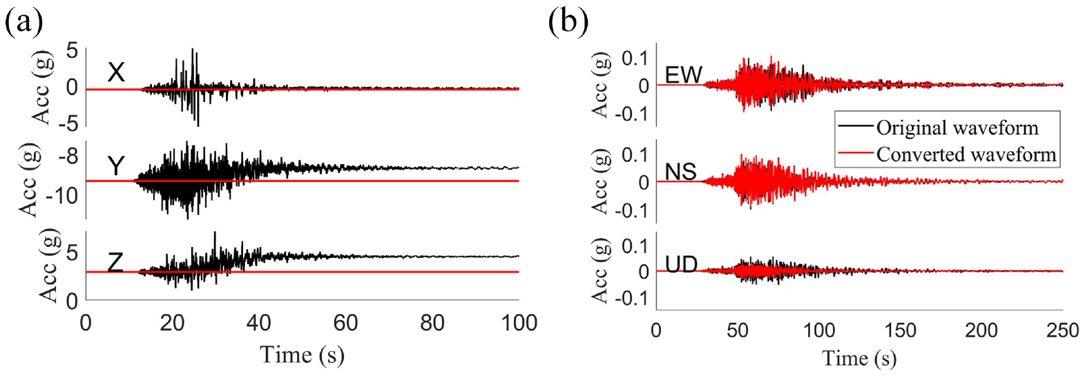
The Mw7.1 off-Fukushima earthquake in 2021: (a) the original waveform of acceleration at station S2N01; (b) The comparison between the original waveform and the converted waveform at station S3N17.
We employed the short-time average over long-time average (STA/LTA) algorithm proposed by Trnkoczy (2002) to extract P-waves and determined noise windows. The filter corner was determined by comparing the Fourier amplitude spectra (FAS) of ground motion records with those of noise windows. Figure 3 illustrates the plot for selecting filter corner frequencies. For the low-pass/high-pass corner frequency (fcLP/fcHP), we used a minimum/maximum signal-to-noise ratio (SNR) equal to 0.5 (Bahrampouri et al., 2021; Boore and Bommer, 2005; Douglas and Boore, 2011).
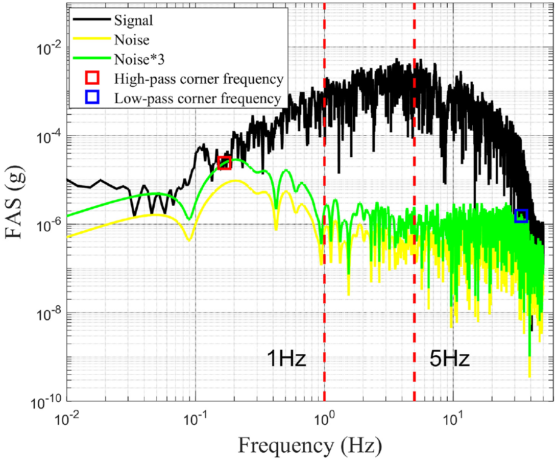
Illustrative plot for selecting the filter corner frequencies.
To achieve the research objectives of this article and account for the model’s influencing factors, the following criteria were used to exclude certain ground motion records in the model’s application:
Records with rotations greater than 0.1° (as shown in Figure 2a).
Records with an SNR less than three for the frequency band of 1∼5 Hz (as shown in Figure 3).
Records with obvious low-quality, such as those with multiple wave packets or missing pre-event memory.
Records with rupture distances greater than 300 km.
Records that do not capture the start of the P-wave.
Records with PGA lower than 1e−3 g.
Records that do not belong to subduction earthquake events, as determined by the method proposed by Zhao et al. (2015). This means that earthquake events are not located near the subduction zone (as shown in Figure 1).
An earthquake with fewer than three records.
The final data set used in this study comprised 5061 sets of three-component records from 194 intraslab earthquakes and 5270 sets of three-component records from 214 interface earthquakes between 2016 and 2023. Figure 4 illustrates the distribution relationship between moment magnitude (M) and rupture distances (Rrup), with the density map of moment magnitude and rupture distance representing the centralized distribution of ground motion data. Rupture distance was calculated using the method proposed by Kaklamanos et al. (2011).
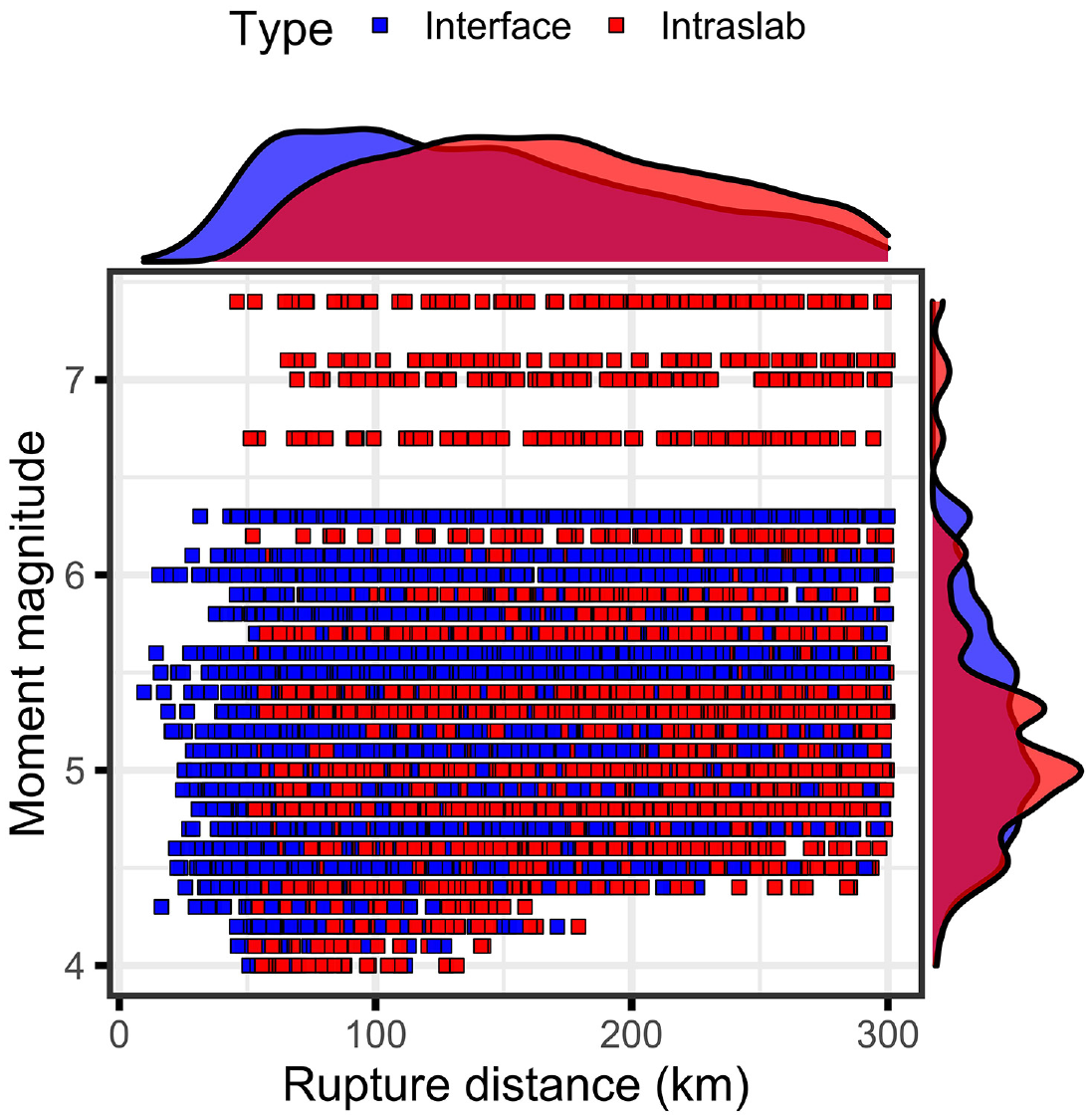
The scatter distribution of ground motion data between moment magnitude (Mw) and rupture distances (Rrup).
The NGA-west2 data processing flow was used for record processing (Ancheta et al., 2014), which included steps such as removing pre-event mean from acceleration, tapering, and padding. The ground motion records used in this article were uniformly processed by baseline correction and fourth-order acausal Butterworth band-pass filter. These records were processed using empirical values for high-pass corner frequencies proposed by Puglia et al. (2018). In contrast, a fixed frequency of 30 Hz was used for the low-pass corner frequency. Douglas and Boore (2011) noted that low-frequency noise (<1 Hz) significantly impacted strong motion intensity parameters, and filtering high-frequency noise was only necessary in specific situations.
Furthermore, the two horizontal components of ground motion used in this study are RotD50 (Boore, 2010), which represents the median ground motion at all rotation angles and is orientation-independent.
Site classification of offshore stations
The estimation of site effect is commonly done using the time-averaged shear-wave velocity over the top 30 m (Vs30, m/s) (e.g. Abrahamson and Gülerce, 2020, 2022; Gregor et al., 2022; Kuehn et al., 2020; Parker et al., 2020, 2022). However, an alternative parameter for site effect estimation is the site predominant period (Tn), which has been increasingly used in recent years (e.g. Kwak and Seyhan, 2020; Zhao and Xu, 2013). VS30 reflects the stiffness of the shallow soil layer and Tn depends on the stiffness of the soil layer and the depth of sediment to the bedrock. Both measurements are associated with site amplification (Arteta et al., 2021; Zhao and Xu, 2013; Zhu et al., 2020).
Due to the lack of Vs30 data for S-net stations, we utilized the horizontal-to-vertical response spectral ratio (HVRSR) with a damping ratio of 5% for each station to classify the sites. To ensure accuracy, we excluded records with PGA greater than 0.05 g, as high-amplitude records may cause nonlinear behavior in the underlying soil (Arteta et al., 2021; Kawase et al., 2019).
The sites were then categorized based on the predominant period (Tn) of each station, resulting in four categories (SC1, SC2, SC3, and SC4). The classification criteria were modified based on the criteria proposed by Idini et al. (2017) and Zhao (2006). The Tn range of site classification was determined using the method proposed by Idini et al. (2017), and the corresponding approximate range of Vs30 was based on the work proposed by Zhao (2006). However, the method of predominant period does not consider the factor of spectral shape. If there are not many records at a station or there are many peaks in the HVRSR, it is difficult to judge according to the predominant period (Tn). To improve the classification accuracy, Zhao (2006) proposed a classification method based on spectral shape index, and Ghasemi et al. (2009) proposed a classification method based on Spearman rank correlation coefficient. The site classification index (SI) was calculated using the method proposed by Ghasemi et al. (2009) to improve the classification accuracy, as follows:

in which n is the total number of periods, di is the difference between the mean HVRSR of the target category and the mean HVRSR for a station. Figure 5 shows the HVRSR curves of some selected stations from S-net. The gray line and black line represent the HVRSR curves of each record and the mean HVRSR curve for a station, respectively.
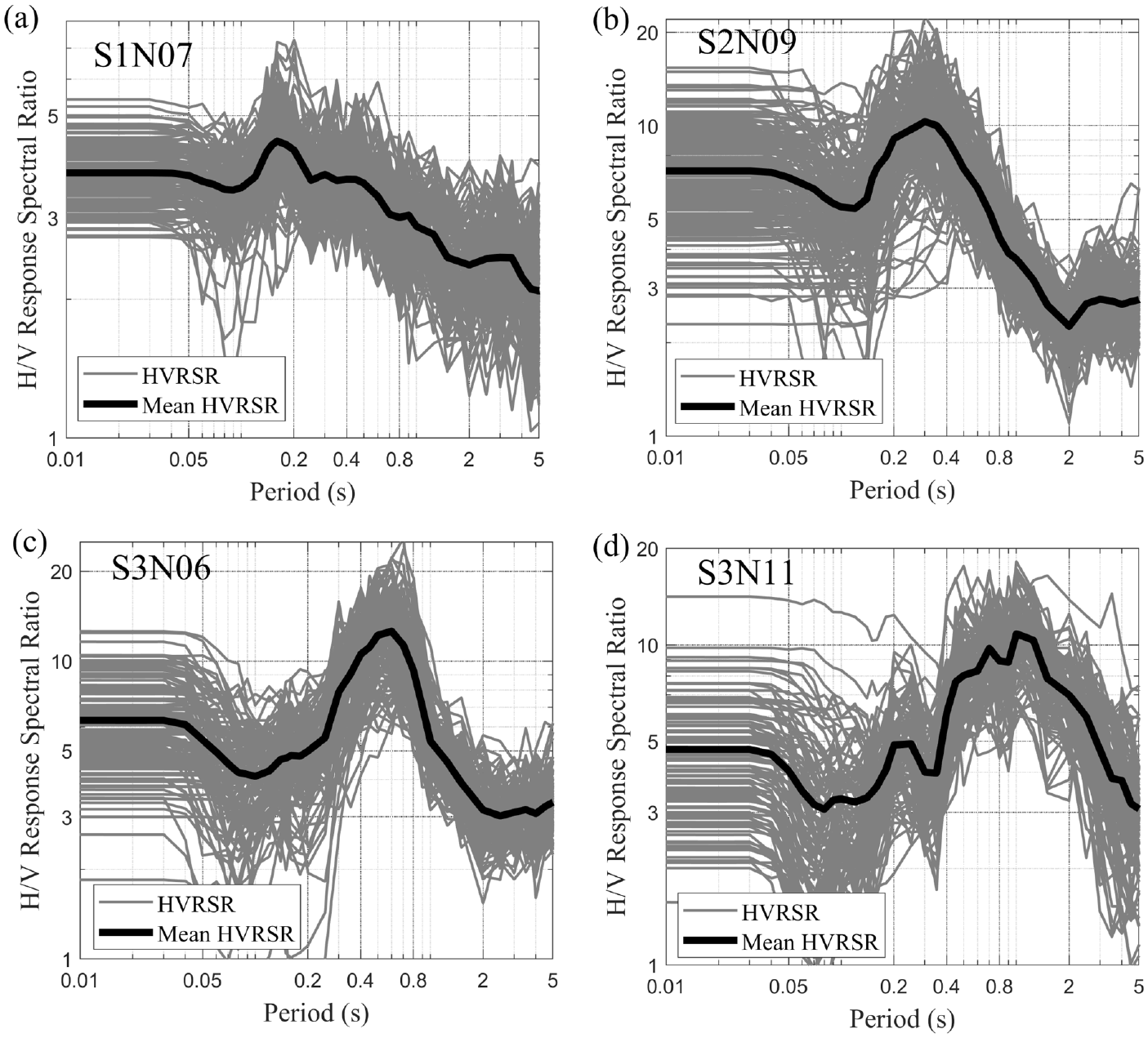
The HVRSR curves of some selected stations: (a) Individual and mean HVRSR curves at station S1N07; (b) Individual and mean HVRSR curves at station S2N09; (c) Individual and mean HVRSR curves at station S3N06; (d) Individual and mean HVRSR curves at station S3N11.
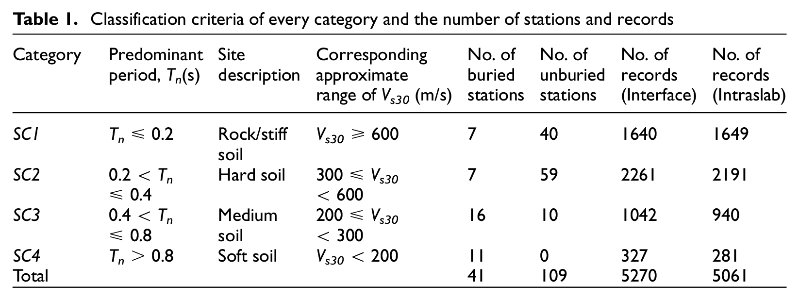
Site categories SC1, SC2, SC3, and SC4 were classified depending on Tn and SI according to Table 1. Table 1 provides the site categories, predominant period ranges, corresponding approximate ranges of Vs30, and the number of stations and records. Figure 6 shows the comparison results of the number of four site categories for buried and unburied stations. The figure shows a more complicated site condition for buried stations than unburied stations (ie., There are four site categories for buried stations and three for unburied stations). The number of unburied stations is mainly distributed in site categories SC1and SC2, whereas the number of buried stations is mainly distributed in site categories SC3 and SC4. This means that most of the unburied stations are located at stiff and hard site conditions, while most of the buried stations are located at medium and soft site conditions.
Classification criteria of every category and the number of stations and records
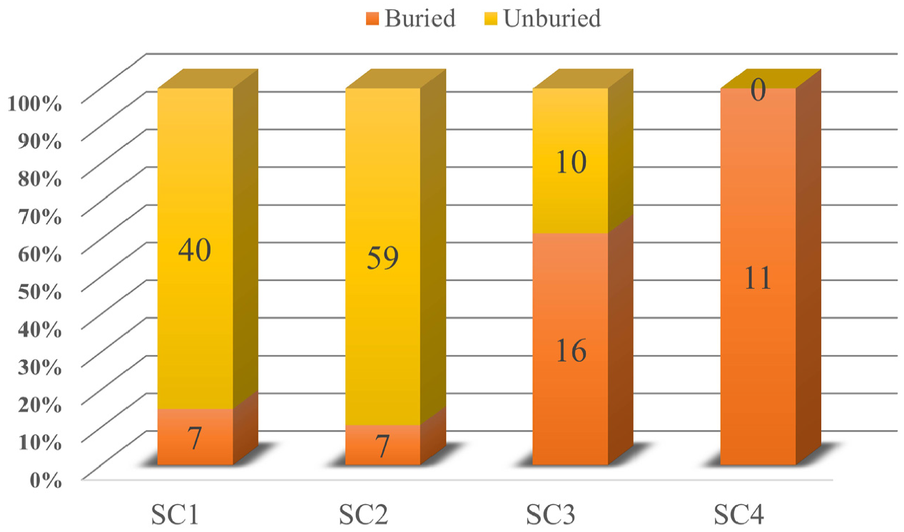
The comparison results of the number of four site categories for buried and unburied stations.
Figure 7 shows the mean HVRSR and the standard deviation (SD) of all stations classified with the predominant period for the site categories SC1, SC2, SC3, and SC4. Figure 7a clearly illustrates that the amplitudes and shapes of the mean HVRSR of the four site categories are significantly different. The mean HVRSR amplitude of unburied stations is greater than that of buried stations. Meanwhile, Figure 7b shows that each of the four site categories has a large SD near the peak amplitude of the mean HVRSR.
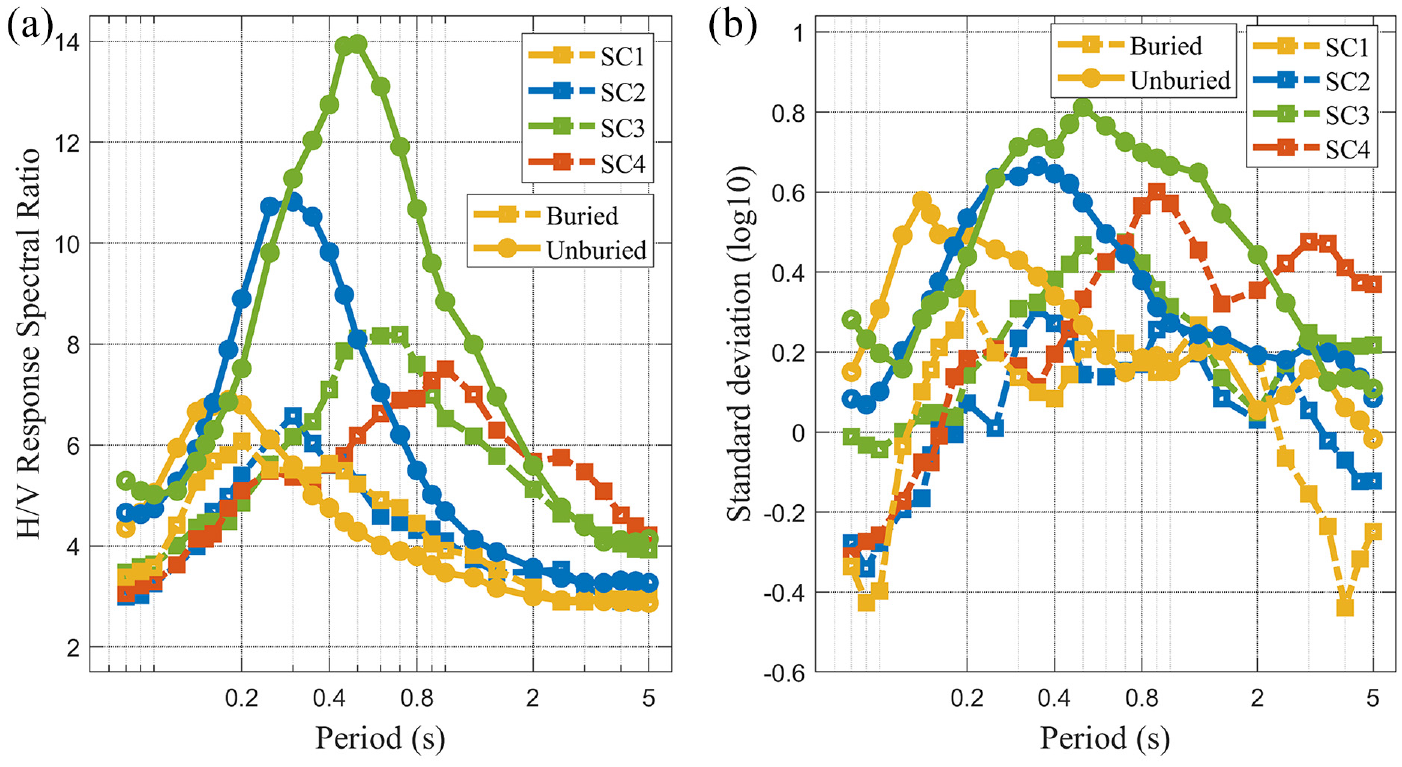
(a) Mean H/V response spectral ratio and (b) corresponding standard deviations for all data from the S-net stations under buried and unburied states for the site categories SC1, SC2, SC3, and SC4.
Figure 8 presents the geographical distribution for the site categories SC1, SC2, SC3, and SC4. Site categories SC1 and SC2 are predominantly located near the Japan Trench, with most of stations being unburied states. On the contrary, site categories SC3 and SC4 are mostly distributed near the onshore, with most of stations being buried states.
The geographical distribution for the site categories SC1, SC2, SC3, and SC4.
Offshore ergodic backbone GMM for subduction earthquakes
The functional form of the ergodic backbone GMM we adopted here is modified based on the functional form of the GMM of Si et al. (2022) for subduction earthquakes. The modified functional form is as follows:

in which A(T) represents the observed ground motion IM, such as PGA and the RotD50 values of 5%-damped spectral acceleration for different periods; M is moment magnitude; Rrup is rupture distance; D is hypocentral depth. δBe is the inter-event residual for eth event and δWes is the intra-event residual for the sth record from the eth event. The residuals δB and δW are uncorrelated and conform to the normal distribution with variances τ2 and ϕ2, respectively.
The b(T) in Equation 2 is the source term, and the functional form adopted is shown in Equation 3. The magnitude scaling contains a linear term and a nonlinear term. Coefficient a0(T) captures the linear scaling associated with magnitude, and coefficient a1(T) captures the nonlinear scaling associated with magnitude. Coefficients d0(T) and d1(T) are the calibrations of earthquake types and are used to reflect differences between interface and intraslab events in GMM. Coefficient e(T) is the constant term.

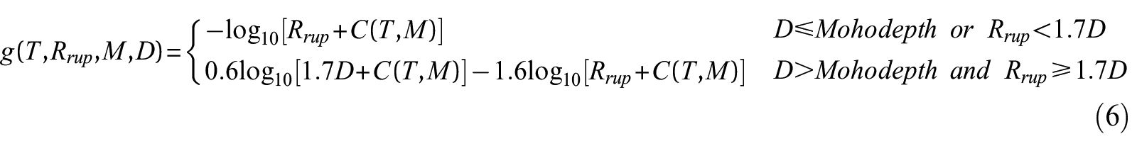
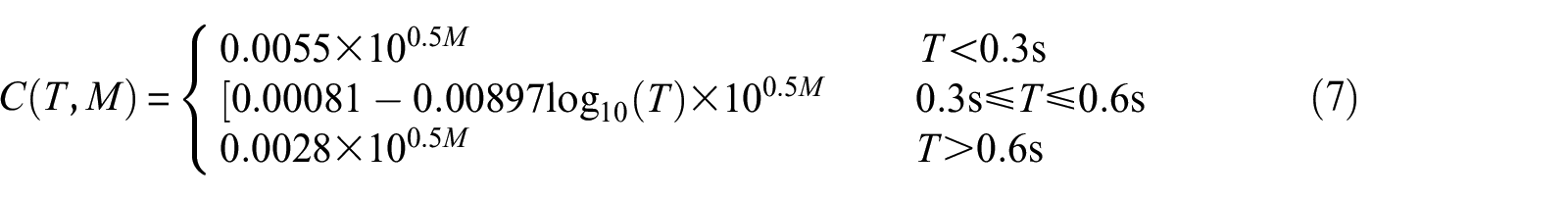
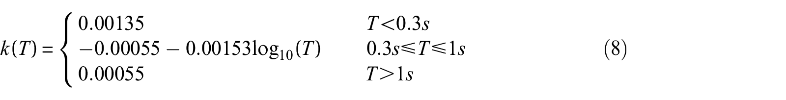
where


The path scaling includes the effect of geometric spreading (log R term) and the anelastic attenuation term (linear R term). The g(T,Rrup, M,D) in Equation 2 is the geometric spreading term, and the k(T)Rrup is the anelastic attenuation term. C(T, M) represents the near-source saturation term associated with period and magnitude changes. The anelastic attenuation coefficient k(T) is modified to capture the offshore ground motion characteristic associated with period. These two terms are correlated in most GMM regressions (Arteta et al., 2021). The geometrical spreading coefficient is used to avoid positive value of the anelastic attenuation coefficient. The data of Moho depth obtained from CRUST 1.0. 1
where
For the estimation of site effects, we introduced a dummy variable (W) with values of 0 and 1 for buried and unburied stations, respectively, as well as each site category in section “Site classification of offshore stations.”Tan and Hu (2023) analyzed the characteristics of offshore ground motion using two largest offshore earthquakes recorded by the S-net. They examined the influence of water column and sediment thickness using residual analysis. Their results showed that the residuals of unburied stations were greater than those of buried stations. Hu et al. (2022a) also found that whether stations are buried or not has a significant influence on the ground motion IM. After residual analysis (see section “Residual analysis of ergodic backbone GMM”), the residuals of spectral acceleration can be evenly distributed around zero with the thickness of sediment layer (D14) and water column, respectively. Therefore, the difference between spectral acceleration and the sediment thickness can be well captured by dividing S-net stations into buried and unburied stations. This means that whether stations are buried or not can be considered as a predictor variable in the ergodic GMM to reflect the influence of water column and the sediment thickness. In addition, several studies showed that site classification can capture the resonant characteristics of a group of sites, allowing adequate description of site amplification on the establishment of GMM (Arteta et al., 2021; Idini et al., 2017; Zhao and Xu, 2013). Based on the above findings, we propose the following functional forms to estimate site effect:

where si is a regression coefficient and i refers to the ith site category.
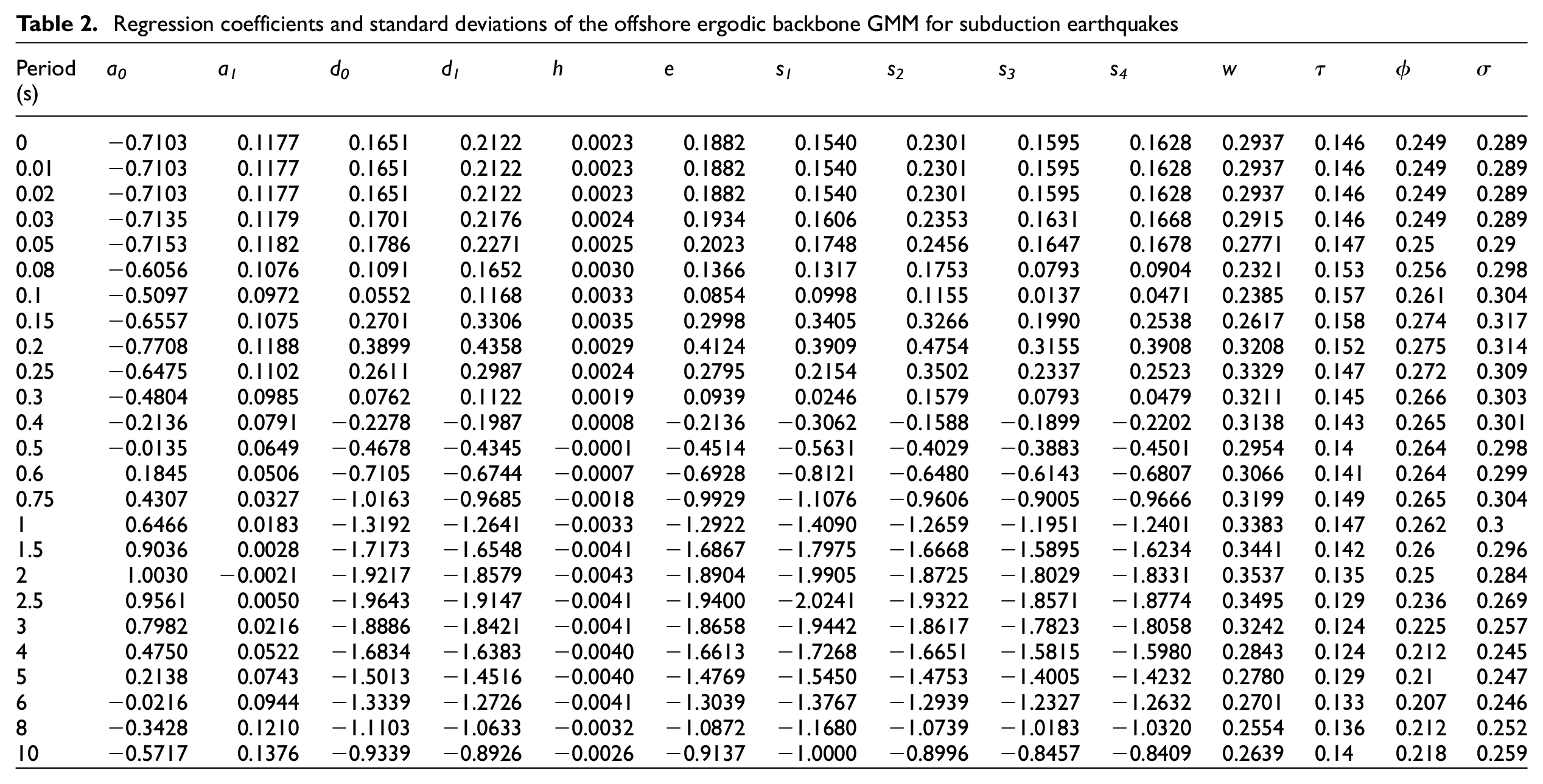
The regression coefficients (a0, a1, d0, d1, h, e, w and si) were determined by mixed-effect regression (Abrahamson and Youngs, 1992; Bates et al., 2015). The regression coefficients and SDs of residuals are presented in Table 2. σ is the total SD of the total residual (δBe + δWes) in Table 2, which can be calculated as
Regression coefficients and standard deviations of the offshore ergodic backbone GMM for subduction earthquakes
Residual analysis of ergodic backbone GMM
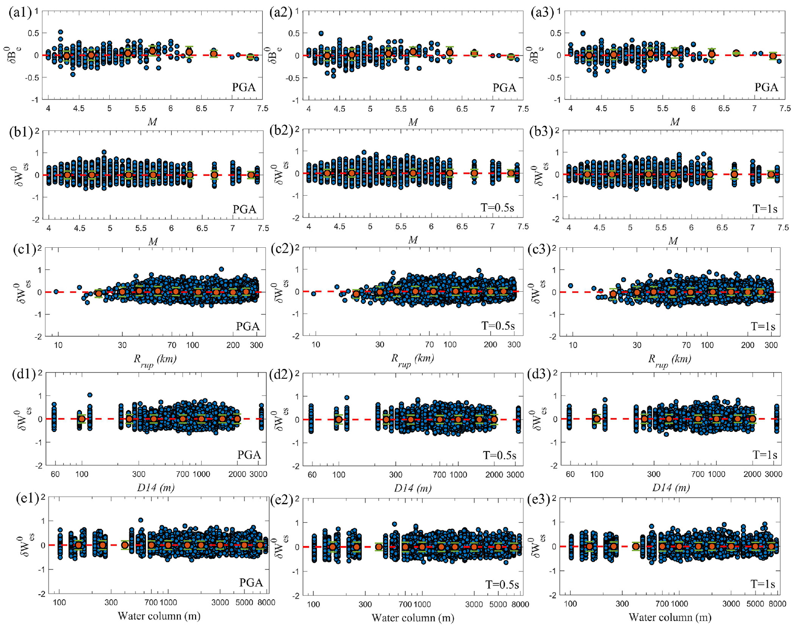
Figure 9 shows residual analysis with respect to moment magnitude (Mw), rupture distance (Rrup), the thickness of sediment up to Vs = 1.4 km/s (D14), and water column for PGA and spectral accelerations at T = 0.5 and 1.0 s. Figure 9a1 to a3 shows the plots of inter-event residuals versus moment magnitude. We note that most of the data correspond to earthquakes with magnitudes less than about 6.5. A possible bias at lager magnitudes is very close to 0; however, the low number of data points within that magnitude range implies that ergodic GMM can capture them. Therefore, these residuals can be considered as epistemic uncertainty for the ergodic GMM due to the lack of data. As may be observed from Figure 9b1 to b3 and Figure 9c1 to c3, the ergodic GMM, in general, is unbiased for all considered magnitude and distance ranges. Ergodic GMM considers whether stations are buried or not as a site predictor variable, and the distribution of the intra-event residuals with respect to the sediment thickness (e.g. Figure 9d1 to d3) and the water column (e.g. Figure 9e1 to e3) are uniformly distributed around zero. This indicates that there is no need to consider water column and sediment thickness as site predictor variables in the ergodic GMM. Figure 10 shows the intra-event residuals with respect to tectonic regime, buried state, and each site category for PGA and spectral accelerations at T = 0.5 and 1.0 s. The residuals and the mean of residuals are centered at zero. This indicates that the ergodic GMM can well reflect the differences of tectonic regime, buried state, and each site category.
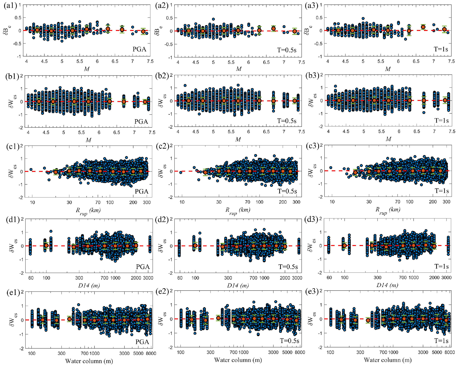
Residual analysis with respect to moment magnitude (Mw), rupture distance (Rrup), the thickness of sediment up to Vs = 1.4 km/s (D14), and water column for PGA and spectral accelerations at T = 0.5 and 1.0 s. (a1)–(a3) the inter-event residuals versus moment magnitude (Mw); (b1)–(b3) the intra-event residuals versus moment magnitude (Mw); (c1)–(c3) the intra-event residuals versus rupture distance (R); (d1)–(d3) the intra-event residuals versus thickness of sediment up to Vs = 1.4 km/s (D14); and (e1)–(e3) the intra-event residuals versus water column. Orange circles and green error bars represent the mean and standard deviation of the residuals, respectively.
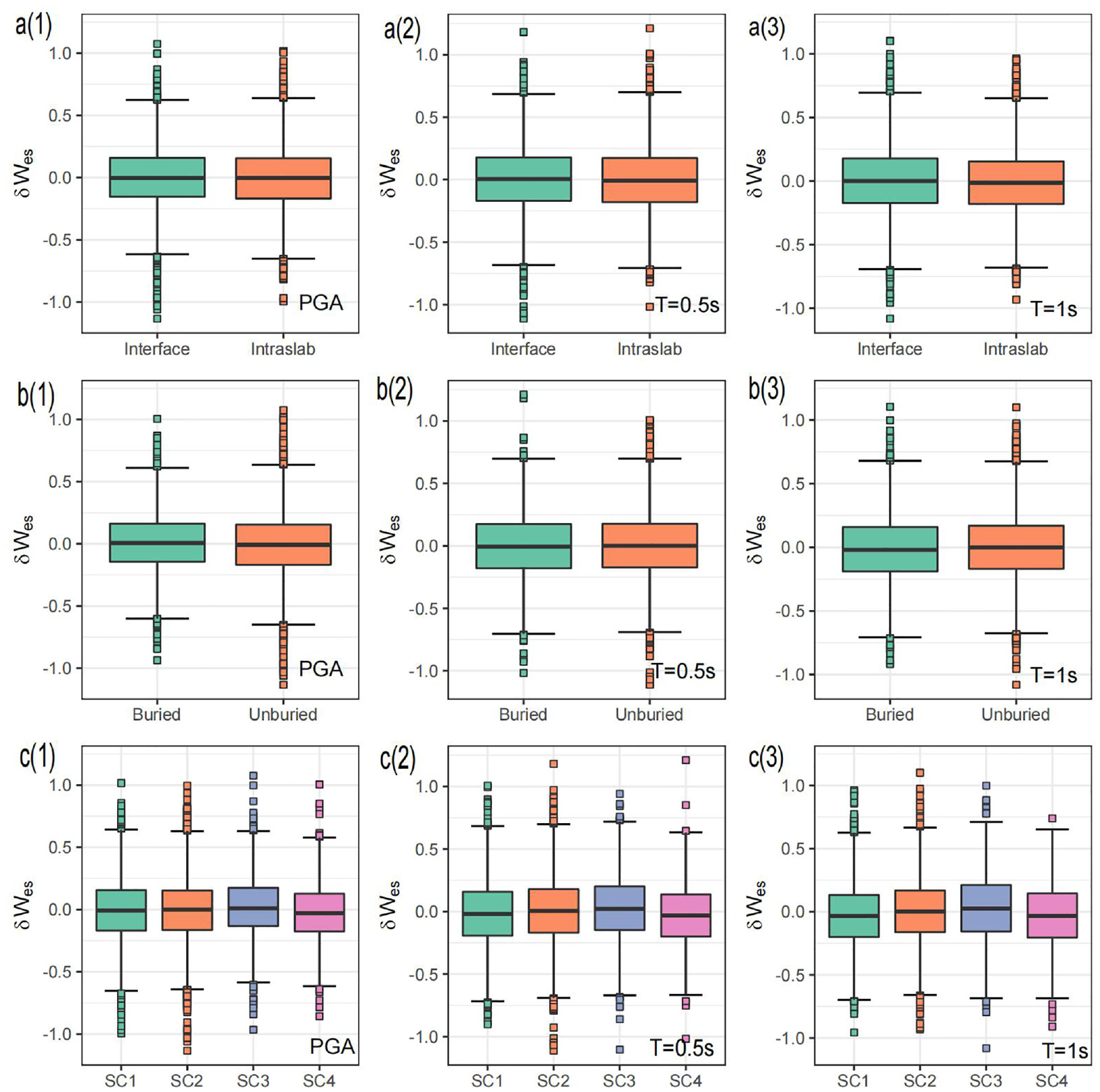
The intra-event residuals with respect to tectonic regime ((a1)–(a3)), buried state ((b1)–(b3)), and each site category ((c1)–(c3)) for PGA and spectral accelerations at T = 0.5 and 1.0 s.
Comparison of offshore ergodic GMM for subduction earthquakes
Figure 11 presents the comparison of median response spectra at different buried states for different site categories with M = 7 and Rrup = 100 km for interface and intraslab earthquakes. For buried stations, the four site categories exhibit varying site amplifications, with peaks occurring at different periods. The generic soil sites (category SC2) exhibit maximum amplification values at T = 0.25 s. Categories SC3 and SC4 spectra exhibit less amplification and a major period shift at the peak, in comparison to category SC1, which corresponds to stiff soil or rock sites. The figure shows that unburied stations show a similar site amplification to the buried stations and a large difference and amplitude for unburied stations.
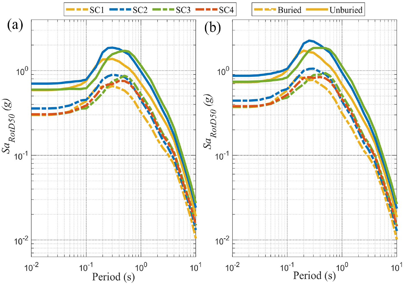
The comparison of median response spectra at different buried states for different site categories with M = 7 and R = 100 km for (a) interface and (b) intraslab earthquakes. D = 30 km for interface earthquakes and D = 50 km for intraslab earthquakes, Moho = 30 km.
Figure 12 shows the comparison of the median response spectra predicted by the offshore ergodic backbone GMM for different hypocentral depths with M = 7 and buried states at a distance of 150 km for interface and intraslab earthquakes, considering a reference site category SC1. The comparison of the median response spectra values for different hypocentral depths shows a large amplitude for deep earthquakes and a stronger depth dependence at shorter periods than at longer periods.
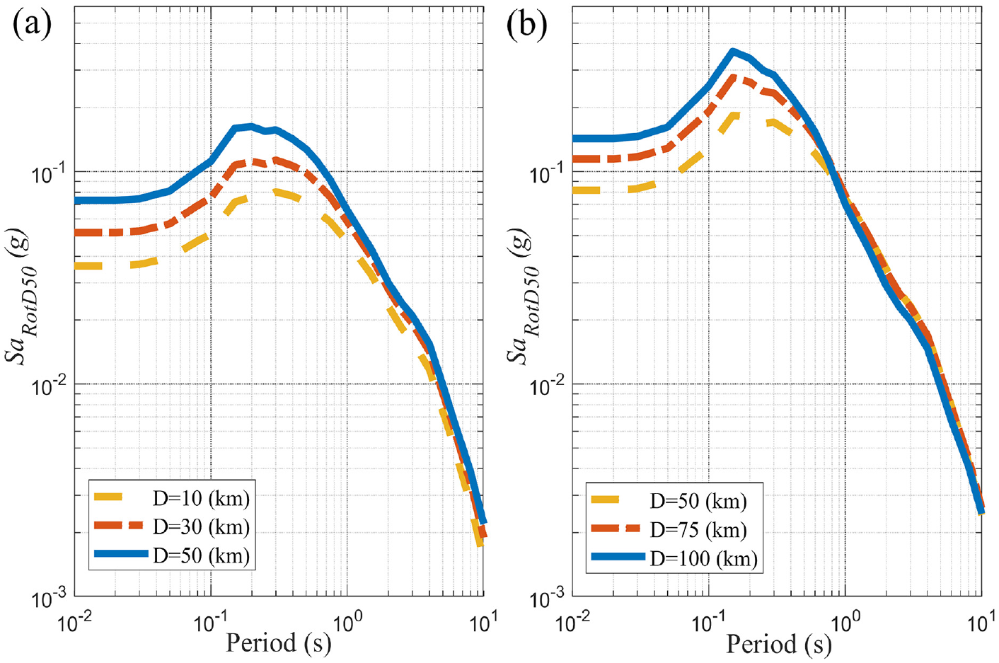
Comparison of the median response spectra predicted by the offshore ergodic backbone GMM for different hypocentral depths with M = 7 and buried states at a distance of 150 km for (a) interface and (b) intraslab earthquakes, considering a reference site category SC1. D = 30 km for interface earthquakes and D = 50 km for intraslab earthquakes; Moho = 30 km.
Figure 13 shows the comparison results of PGA and SaRotD50 (T = 1 s) attenuation curves at different M values and buried states predicted by the offshore ergodic backbone GMM for interface and intraslab earthquakes with a reference site category SC1. This figure shows a clear amplitude-saturation for lager magnitude events at short distance and a strong M dependence at different periods. The amplitude of intraslab events at the same magnitude is greater than that of interface events and unburied stations show a larger amplitude than buried stations. The comparison of PGA and SaRotD50 (T = 1 s) attenuation curves for smaller earthquake events shows a steeper attenuation with distance than for larger earthquake events.
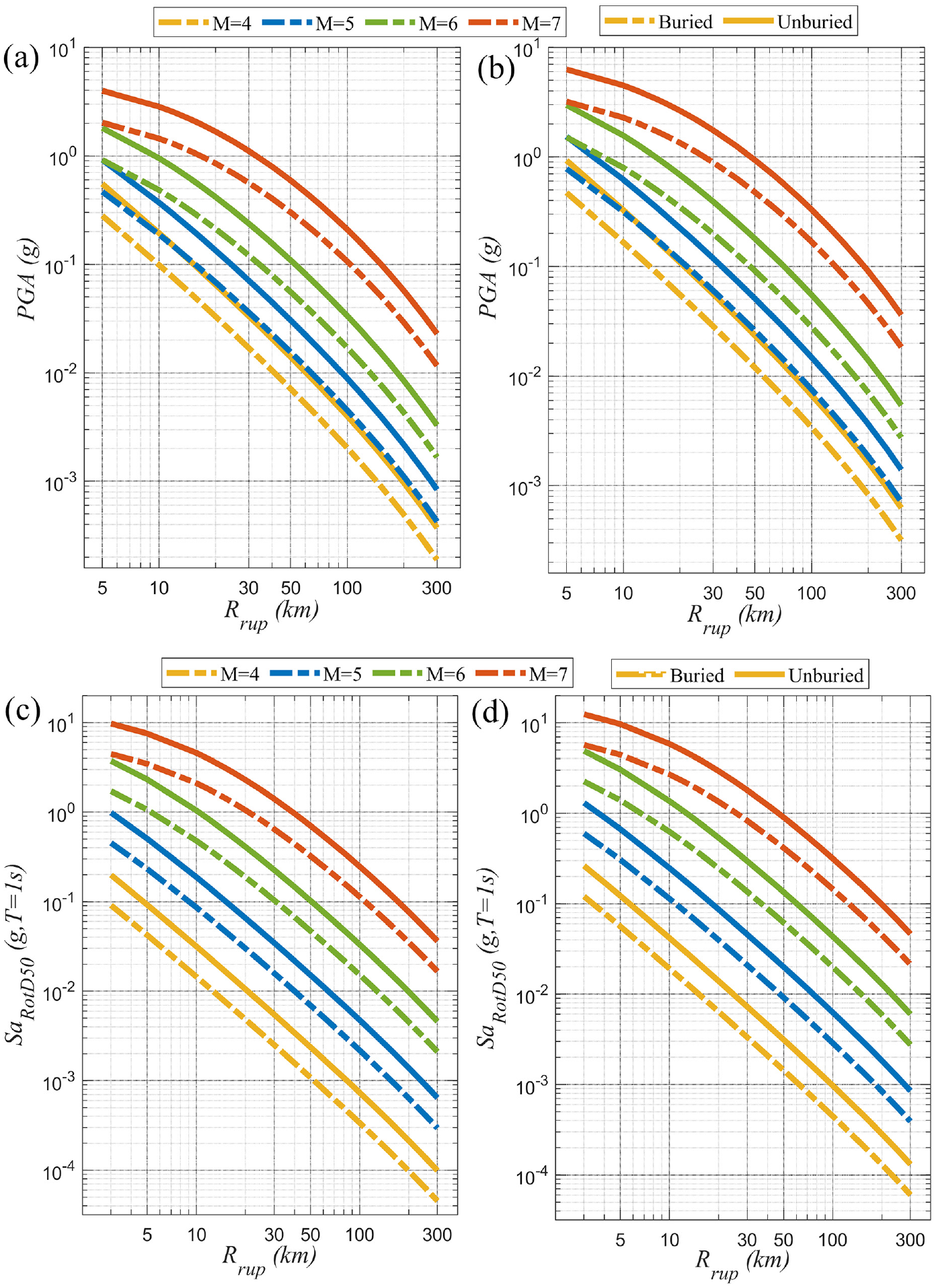
The comparison results of ((a) and (b)) PGA and ((c) and (d)) SaRotD50 (T = 1s) attenuation curves at different M values and buried states predicted by the offshore ergodic backbone GMM for interface (left panel) and intraslab (right panel) earthquake events with a reference site category SC1. D = 30 km for interface earthquakes and D = 50 km for intraslab earthquakes; Moho = 30 km.
Figure 14 shows the comparison results of median response spectra at different M values and buried states predicted by the offshore ergodic backbone GMM at Rrup = 60 km and Rrup = 120 km for interface and intraslab earthquakes with a reference site category SC1. The figure shows the intraslab earthquakes have lager amplitude than interface ones at the same rupture distance, and the long-period attenuation become slower as M increases. The amplitude of median response spectra decreases as Rrup increases.
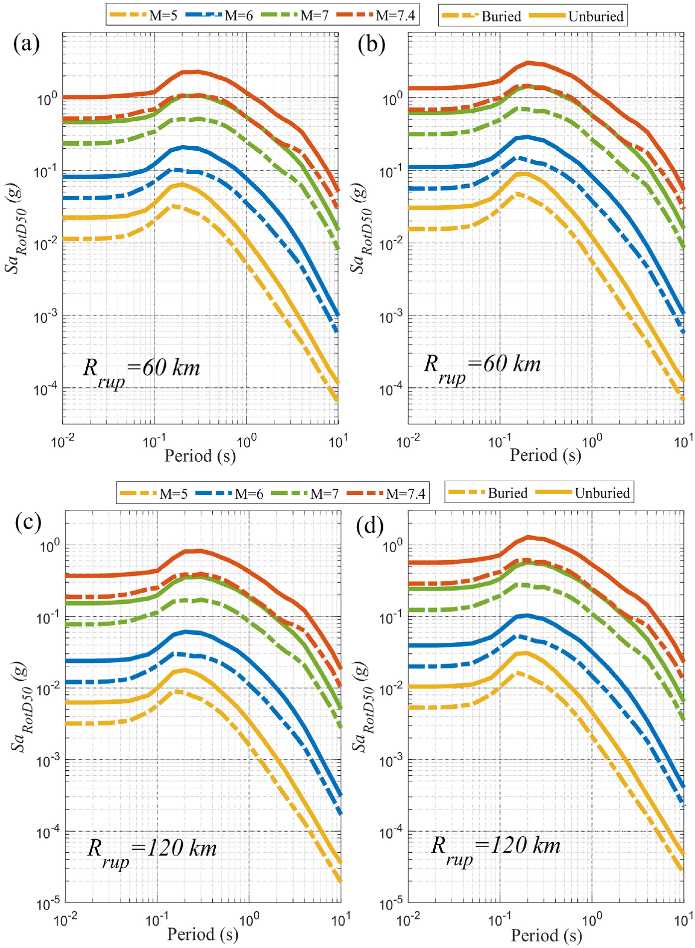
The comparison results of median response spectra at different M values and buried states predicted by the offshore ergodic backbone GMM at ((a) and (b)) Rrup = 60 km and ((c) and (d)) Rrup = 120 km for (left panel) interface and (right panel) intraslab earthquakes with a reference site category SC1. D = 30 km for interface earthquakes and D = 50 km for intraslab earthquakes; Moho = 30 km.
In recent years, two of the largest offshore subduction-slab earthquakes (February 13, 2021, M 7.1 and March 17, 2022, M 7.4) have caused significant damage to onshore structures. Figure 15a and b compare the offshore ground motion of the 2022 M7.4 off-Fukushima earthquake recorded by S-net with the median values predicted by the offshore ergodic backbone GMM for PGA and SaRotD50 (T = 1 s). The PGA and SaRotD50 (T = 1 s) of offshore ground motion are significantly different between the buried and unburied states. The offshore ergodic backbone GMM captures the characteristics of the offshore ground motion well in terms of distance scaling, both in buried and unburied states. Figure 15c and d compare the offshore ground motion of the 2021 M 7.1 off-Fukushima earthquake with the median values predicted by the offshore ergodic backbone GMM for PGA and SaRotD50 (T = 1 s). Note that the offshore ergodic backbone GMM is developed based on data less than 300 km, but the ergodic GMM in Figure 15 demonstrates that it is still somewhat predictive for data greater than 300 km. In addition, the PGA attenuation curves of buried and unburied states exhibit consistent attenuation with observation data greater than 300 km. However, there are some differences between the SaRotD50 (T = 1 s) attenuation curves of buried and unburied states and observed ground motion data greater than 300 km. For SaRotD50 (T = 1 s) observation data, ground motion data of unburied stations exhibits faster attenuation beyond 300 km, while ground motion data of buried stations exhibits slower attenuation. This may be due to the increased ground coupling caused by buried stations, resulting in slow attenuation at long-period and long-distance.
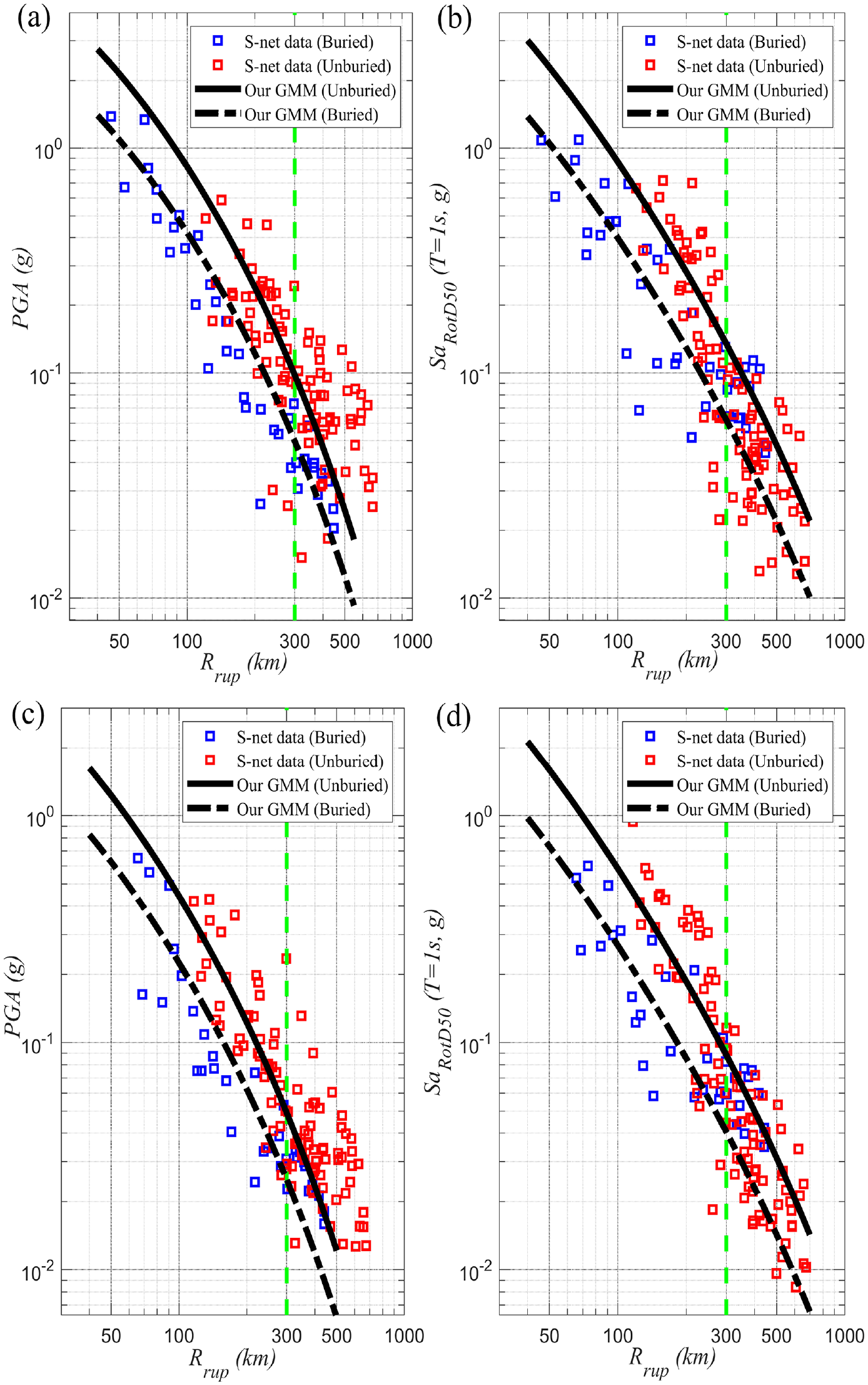
The comparison of offshore ground motion recorded by S-net with median values predicted by the offshore ergodic backbone GMM at PGA (left panel) and SaRotD50 (T = 1 s) (right panel) for ((a) and (b)) 2022 M7.4 off-Fukushima earthquake and ((c) and (d)) 2021 M 7.1 off-Fukushima earthquake with a reference site category SC1.
Comparison of the proposed GMM with previous studies for subduction earthquakes
We compared the ergodic GMM with NGA-Sub GMMs (e.g. Abrahamson and Gülerce, 2020, referred to as AG20; Parker et al., 2020, referred to as PSBAH20; Si et al., 2020, referred to as SMK20) and some subduction GMMs from Japan (e.g. Zhao et al., 2016a, referred to as Zea16; Zhao et al., 2016b, referred to as Zea16; Hu et al., 2020, referred to as HTZ20). Note that the HTZ20 is a single-station offshore GMM based on onshore and six offshore stations, and we choose the mean values of the six offshore stations for comparison. For the NGA-Sub GMMs, the magnitude scaling breakpoint values for the Japanese Pacific tectonic plates are plotted. The median values predicted by the offshore ergodic backbone GMM are presented at buried and unburied states for interface and intraslab earthquakes with a reference site category SC2. The comparison results of PGA and spectral acceleration at period of 1 s (Sa(T = 1 s)) attenuation curves are presented for interface and intraslab events with magnitude 7 for the defined site condition with Vs30 values of 500 m/s, which corresponds to the Vs30 range for the site category SC2. For the response spectra, the comparison results are provided at two distances of 75 and 200 km for interface and intraslab events with magnitude 7. Note that the Zea16 and HTZ20 are developed using the geomean horizontal component, whereas the NGA-Sub GMMs and our ergodic GMM are developed using the RotD50 horizontal component. For the distance scaling, the Zea16 and HTZ20 use the hypocentral distance, while our ergodic GMM and the NGA-Sub GMMs use the rupture distance. The comparison is a general comparison between our offshore ergodic GMM and other GMMs for subduction earthquakes, without using spectral period-dependent scaling (Boore and Kishida, 2017) to adjust the geometric horizontal component to the RotD50 component (Gregor et al., 2022), and without adjusting on the distance scaling.
Figure 16 shows the comparison results of PGA and Sa (T = 1 s) attenuation curves for interface and intraslab events with magnitude 7. Figure 16a and b shows the comparison results of PGA attenuation curves for interface and intraslab events. The offshore ergodic GMM and HTZ20 show a smaller difference in amplitude because the HTZ20 is developed based on data from six offshore stations and is able to represent the offshore ground motion of PGA. For the interface events, the amplitude of the PGA attenuation curve of the offshore GMM is larger than that of the NGA-Sub GMMs. In contrast, for intraslab events, the differences between the PGA attenuation curves of offshore GMM for the buried states and the PGA attenuation curves of onshore GMMs are relatively small. However, there are still significant differences between the PGA attenuation curves of offshore GMM for the unburied states and the PGA attenuation curves of onshore GMMs. Figure 16c and d shows the comparison results of Sa (T = 1 s) attenuation curves for interface and intraslab events. The Sa (T = 1 s) attenuation curves of the offshore GMM for buried and unburied states show a lager amplitude and a steeper attenuation than those of the NGA-sub GMMs.
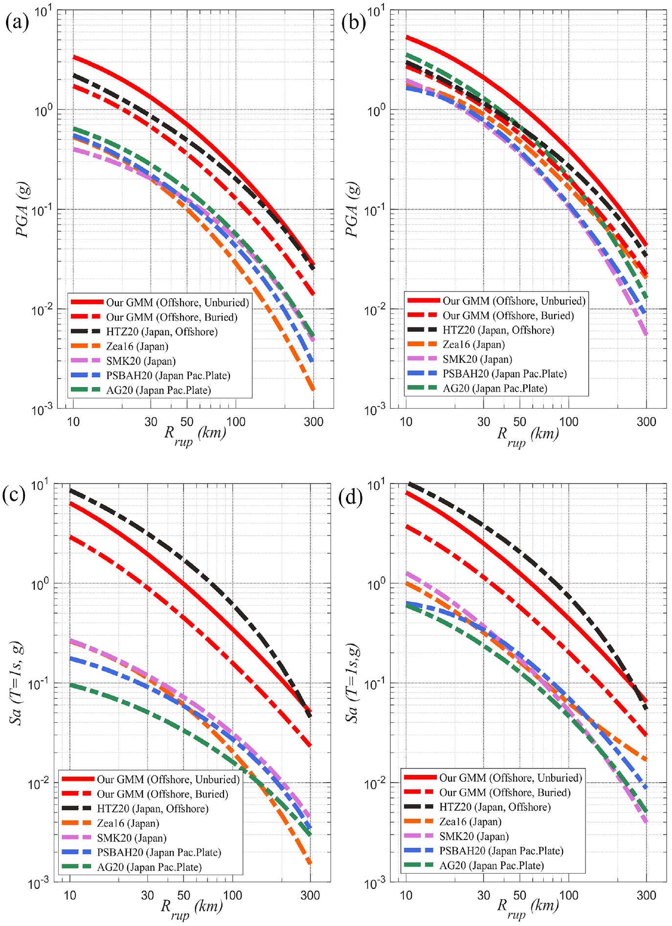
The comparison results of ((a) and (b)) PGA and ((c) and (d)) Sa (T = 1 s) attenuation curves for interface (left panel) and intraslab (right panel) events with magnitude 7 and a reference site category SC2. For NGA-Sub GMMs, Ztor = 10 km for interface events and Ztor = 50 km for intraslab events; hypocentral depth (ZHYP) is 30 km for interface events and hypocentral depth is 50 km for intraslab events; Vs30 = 500 m/s.
Figure 17a and b shows the comparison results of response spectra for interface and intraslab events with magnitude 7 at a distance of 75 km. The offshore ergodic GMM with unburied states exhibits similar trends to the HTZ20 at short periods, but still has some differences at long periods. For interface events, the difference between offshore GMMs and onshore GMMs becomes larger as period increases. For intraslab events, the offshore ergodic GMM with buried states shows a similar trend to NGA-sub GMMs at short periods. However, the difference between offshore GMMs and onshore GMMs increases as period increases, which is similar to the trend of interface events. Figure 17c and d shows the comparison results of response spectra for interface and intraslab events with magnitude 7 at a distance of 200 km. The offshore ergodic GMM and HTZ20 show great similarity in amplitude and trend, especially for the unburied states. For interface events, the offshore ergodic GMM are still dramatically different from the NGA-sub GMMs, with differences similar to the response spectra at 75 km. For intraslab events, the comparison results are similar to those of the response spectra at a distance of 75 km. These comparisons demonstrate that offshore GMMs are significantly different from onshore GMMs for subduction earthquakes, especially in the long-period and unburied states. Furthermore, the larger period of the peak response spectra of offshore GMMs compared to onshore GMMs implies that offshore ground motions are characterized by rich long-period ground motion.
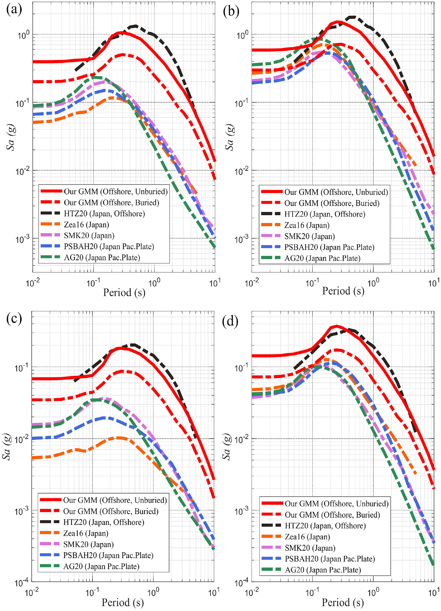
The comparison results of response spectra for interface (left panel) and intraslab (right panel) events with magnitude 7 at a distance of ((a) and (b)) 75 km and ((c) and (d)) 200 km with a reference site category SC2. For NGA-Sub GMMs, Ztor = 10 km for interface events and Ztor = 50 km for intraslab events; hypocentral depth (ZHYP) is 30 km for interface events and hypocentral depth is 50 km for intraslab events; Vs30 = 500 m/s.
The significant differences in attenuation curves and response spectra between offshore and onshore models highlight the impracticality of directly applying onshore GMMs to offshore areas. Therefore, it is necessary to develop reasonable prediction models for offshore ground motion based on offshore ground motion observed data, particularly for subduction earthquake events that can cause significant damage. The large differences between onshore and offshore GMMs may be attributed to various factors, such as the deployment method of the seafloor stations, the degree of coupling between the stations and the seafloor, the topography of the seafloor, the thickness of the seafloor sediment, and the depth of seawater (Cui et al., 2023; Dhakal et al., 2021; Tan and Hu, 2023). Furthermore, the significant differences between buried and unburied stations suggest that the attenuation curves and response spectra of unburied stations are more susceptible to the influence of complex seafloor environments. In comparison, offshore buried stations increase the coupling with the seafloor, resulting in less difference in attenuation curves and response spectra between buried stations and onshore stations. However, some differences still exist due to the influence of seafloor topography and other factors.
Development of offshore non-ergodic GMM for subduction earthquakes
The development of non-ergodic GMM is based on an ergodic GMM to account for systematic and repeatable source, site, and path effects. We briefly describe the development of the non-ergodic GMM, using functional forms similar to Abrahamson et al. (2019), Kuehn et al. (2019), and Macedo and Liu (2022). We use the offshore ergodic backbone GMM with adjustment terms to describe the offshore non-ergodic GMM, which can be written as:


where μergdic(x) represents the median value of ground motion IMs estimated from the ergodic backbone GMM (e.g. Equation 1). δc0 is the constant intercept indicating the change in weight of each record due to the non-ergodic model considering spatial correlation. δL2 L(te), δS2 S(ts) and δP2 P(te, ts)) are systematic and repeatable source, site and path effects, respcetively, which are epistemic uncertainties that cannot be represented by ergodic GMM; and te and ts are the earthquake (epicenter) and station coordinates in the geography. δceq(te) term is the spatially varying source-specific adjustment term, which is intended to capture spatially correlated and repeatable source effects. δcstat(ts) is the spatially varying site adjustment term, which is intended to capture the repeatable regional site effects. δS2S0 is the spatially location-specific site adjustment, which captures the repeatable location-specific site effects. δB0
e
, δW0
es
, and δS2S0 are the inter-event, intra-event, and site-to-site residuals of non-ergodic GMM, which conform to the normal distribution of N(0, τ02), N(0, ϕ02), and N(0, ϕs2s02), respectively. θattenR is the anelastic attenuation function in the offshore ergodic backbone GMM;
The cell-specific anelastic attenuation method
The cell size of 20 km × 20 km provides a good coverage for the Japan Trench region using the cell-specific anelastic attenuation method proposed by Dawood and Rodriguez-Marek (2013). The Cohen–Sutherland algorithm is used to calculate the path length Ri through each cell, which is a line clipping algorithm used in computer graphics (Foley et al., 1994; Liu et al., 2022a; Macedo and Liu, 2022). The algorithm was first proposed by Foley et al. (1994) and then extended by Liu et al. (2022a). The algorithm effectively determines whether a specific propagation path passes through a cell, avoiding unnecessary Ri calculations when the path does not pass through certain cells. Figure 18a shows the schematic diagram of the propagation path of seismic wave from the epicenter to the station (ray path diagram (green line)). A total of 2052 cells of 20 km × 20 km size was covered in the Japan Trench region using the cell-specific anelastic attenuation method, of which 931 cells contained propagation paths as shown in Figure 18b. In addition, the number of paths in cells contains at most 1285 paths and at least 1 path.
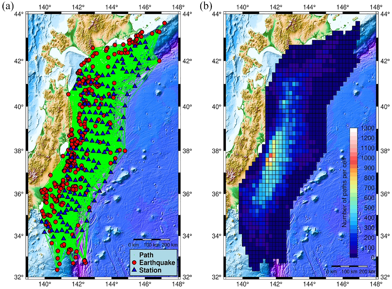
(a) The schematic diagram of the propagation path and (b) the generated grid cells covered the Japan Trench region and the number of paths passed by each cell. The epicenters and stations are shown with red dots and blue triangles, respectively.
Bayesian inference with the integrated nested Laplace approximation
Bayesian inference provides a method to solve the uncertainty of the model by using probability theory, which can model the uncertainty of the non-ergodic GMM as probability distribution (Liu et al., 2022a, 2022b; Macedo and Liu, 2022). The integrated nested Laplace approximation (INLA) method can be implemented using the R-INLA package (www.r-inla.org) in the R computing environment (Lindgren and Rue, 2015; Rue et al., 2017). The INLA method, proposed by Rue et al. (2009), is a computationally effective alternative to Markov chain Monte Carlo designed for latent Gaussian models (Lindgren and Rue, 2015). For an introduction to INLA theory and example models, you can refer to works such as Blangiardo and Cameletti (2015), Wang et al. (2018), Krainski et al. (2019), and Gómez-Rubio (2020). The specific process of INLA is as follows: (1) a latent Gaussian random field (GRF) is used for modeling in a region of interest. (2) The finite-element method is used to divide the spatial domain into a group of disjoint triangles, and the latent GRF is represented as the latent Gaussian Markov random field (GMRF). (3) The latent GMRF with Matérn covariance matrices is used as solutions to stochastic partial differential equations (SPDEs) (Lindgren and Rue, 2015).
The spatially varying source and site adjustment (δceq(te) and δcstat(ts)) in the non-ergodic GMM are modeled as a Gaussian process with mean zero and Matérn covariance function (also known as the kernel function) (Landwehr et al., 2016; Macedo and Liu, 2022), as follows:


where k(·,·) is a covariance function that determines the spatial correlation of systematic and repeatable source and site effects at any two locations; ψ is a hyperparameter that represents the marginal SD of the space field, Г(υ) is the gamma function, Kυ is the modified Bessel function of the second kind, κ is a scale parameter and υ is a smoothness parameter.
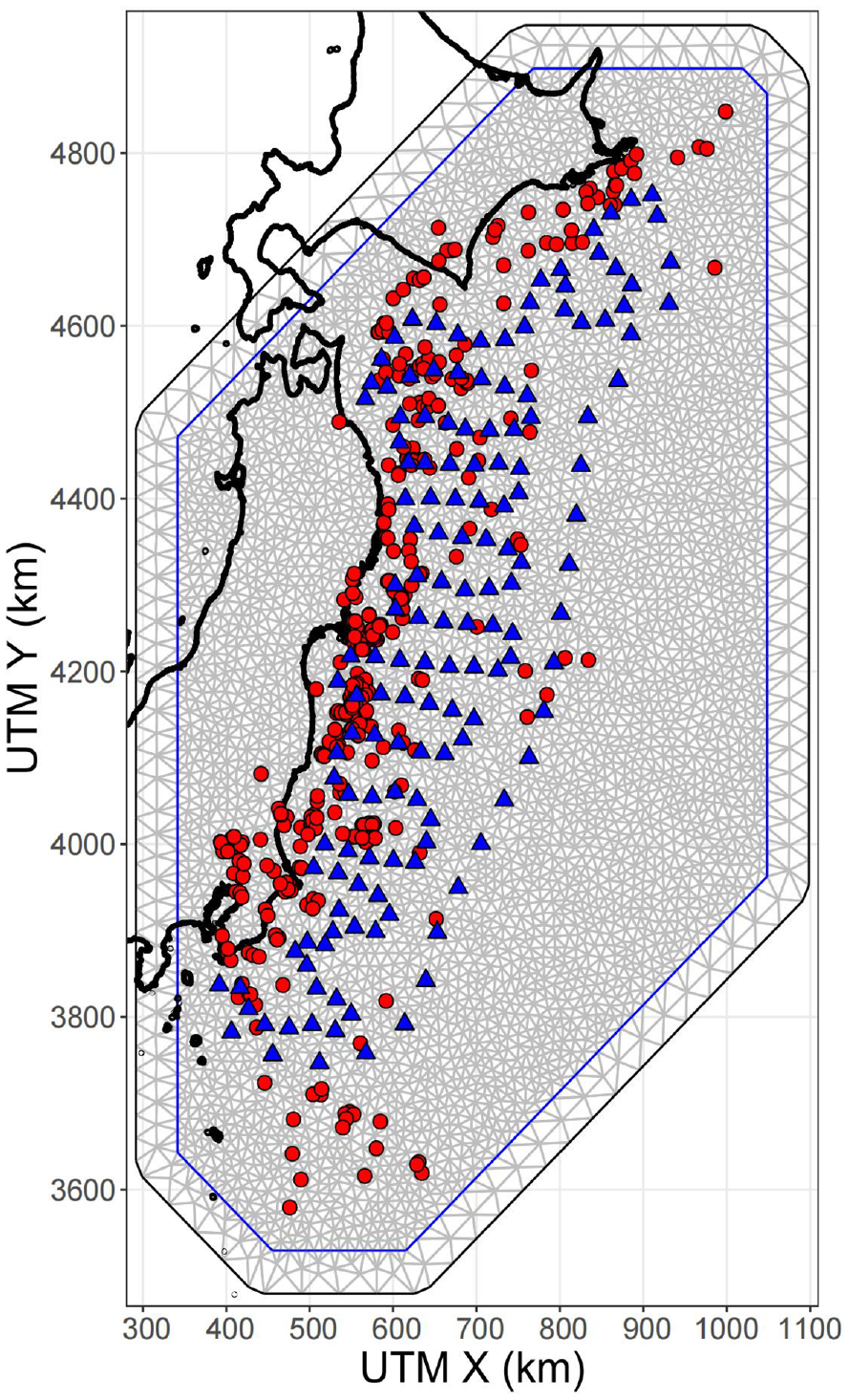
The triangular grid generated by the integrated nested Laplace approximation (INLA) method. The epicenters and stations are shown with red dots and blue triangles, respectively.
INLA is a Bayesian method, which means that a prior distribution for the estimated parameters needs to be set first. The parameters include: fixed effects (δc0); SDs of offshore non-ergodic GMM (τ0, ϕ0 and ϕs2s); and hyperparameters for the spatially varying term (e.g. spatial range ρ and SD ψ). To represent the prior distribution of fixed effects, the following normal distribution is used:

The prior distributions of the SD τ0, ϕ0, and ϕs2s0 use a log-gamma distribution with a shape parameter of 0.9 and a rate parameter of 0.01:
The prior distribution of hyperparameters for spatially varying terms is based on the penalized complexity (PC) prior proposed by Fuglstad et al. (2019) for the SPDE model. The PC prior aims to shrink the parameters toward a simpler base model where the spatially varying terms have zero marginal variance and infinite range. For further details, you can refer to works such as Fuglstad et al. (2019) and Franco-Villoria et al. (2019). The spatial range ρ of the spatially varying term is specified with a prior probability of 50% for a spatially varying term smaller than 30 km; the SD ψ of the spatially varying term is specified with a prior probability of 1% for a spatially varying term larger than 0.3:
In addition, the scale of anelastic attenuation coefficient ci is very different, and we also use the PC prior for the prior distribution of its SD:

Results of offshore non-ergodic GMM
Spatially varying coefficient term
Figures 20 and 21 show maps of spatially varying source and site coefficient term (ie., δceq and δcstat values) calculated by the INLA method, and the output results contain the mean, quartile values, and SD of the marginal posterior distribution. Positive values in the map indicate that the systematic and repeatable source and site effects in the region are higher than the average level; negative values indicate that the source and site effects are lower than the average level.
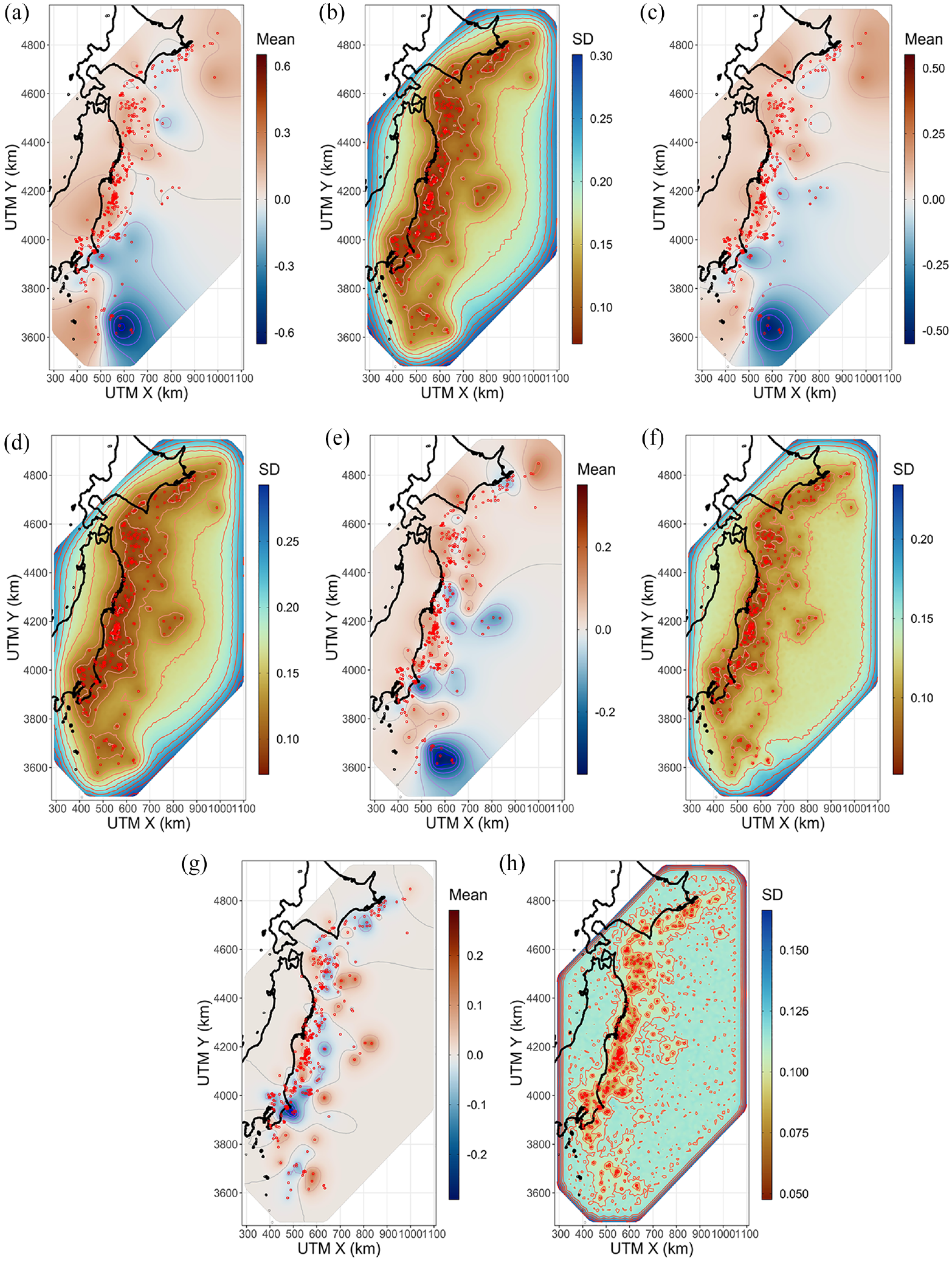
(a) the mean values of source effects for PGA; (b) the standard deviations of source effects for PGA; (c) the mean values of source effects for SaRotD50 (0.5 s); (d) the standard deviations of source effects for SaRotD50 (0.5 s); (e) the mean values of source effects for SaRotD50 (1 s); (f) the standard deviations of source effects for SaRotD50 (1 s); (g) the mean values of source effects for SaRotD50 (8 s); (h) the standard deviations of source effects for SaRotD50 (8 s). In plots, the red dots represent the epicenters.
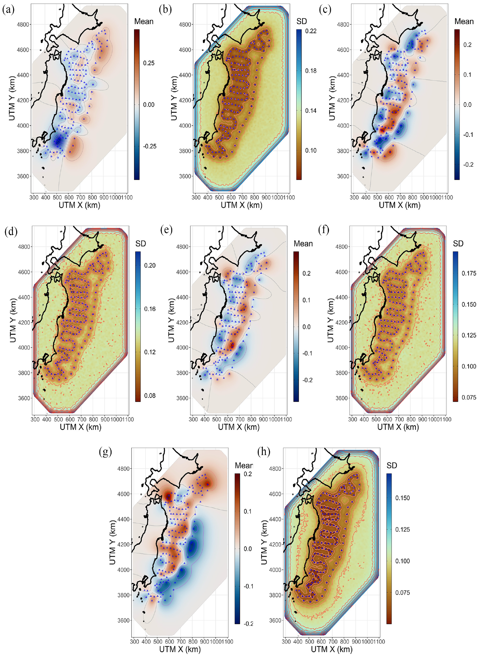
The mean and standard deviation (SD) of the spatially varying site effects for PGA and spectral accelerations at T = 0.5, 1.0, and 5.0 s: (a) the mean values of site effects for PGA; (b) the standard deviations of site effects for PGA; (c) the mean values of site effects for SaRotD50 (0.5 s); (d) the standard deviations of site effects for SaRotD50 (0.5 s); (e) the mean values of site effects for SaRotD50 (1 s); (f) the standard deviations of site effects for SaRotD50 (1 s); (g) the mean values of site effects for SaRotD50 (5 s); and (h) the standard deviations of site effects for SaRotD50 (5 s). In plots, the blue triangles represent the distribution of stations.
Figure 20 shows maps of the mean and SD of the spatially varying source effects (δceq) for PGA and spectral accelerations at T = 0.5, 1.0, and 8.0 s. Figure 20a, c, e and g reveal that the positive values of the spatially varying source effects are predominantly concentrated on the side adjacent to the coast, while the negative values are primarily dispersed on the offshore side. Moreover, both positive and negative values are clustered near fixed locations and do not vary greatly with the period. This indicates that the subduction earthquakes happened on the coastal side are endowed with a greater potential for destruction in the Japan trench area. The INLA method takes the spatial correlation length into account and controls the attenuation of the correlation with the separation distance. Therefore, the map shows non-zero mean values for some locations where no earthquakes occurred. In addition, the spatial pattern exhibited by the spatial varying source effects indicates that the spatial correlation length varies greatly in different periods. The Table 3 shows the values of hyperparameter ρ for different periods controlling the range of spatial correlation length of spatially varying terms. Figure 20 and Table 3 show a lager spatial correlation length of spatially varying source effect at shorter periods than at longer periods. The spatially varying source effects exhibit different spatial patterns due to the nature of the ground motion parameters. The short-period parameters are sensitive to high-frequency ground motion, while the long-period parameters are sensitive to low-frequency ground motion. This difference in frequency content can lead to different spatial patterns of spatially varying source effects. The shorter correlation length for long-period parameters might be related to the attenuation of high-frequency ground motion with distance. High-frequency ground motion attenuates more rapidly than low-frequency ground motion, which can result in shorter correlation lengths for long-period parameters. This is because the energy of high-frequency waves is absorbed more quickly by the Earth’s crust, resulting in more localized effects. Figures 20b, d, f, and h indicates that the locations where historical earthquakes occurred exhibit a smaller SD. Conversely, the locations where no historical earthquakes occurred display near-zero mean values and large SDs, implying that there is insufficient data to constrain the systematic and repeatable source effect.
The mean values of the posterior distributions of the hyperparameters and the inter-event, intra-event, site-to-site, and total aleatory standard deviations for the non-ergodic GMM
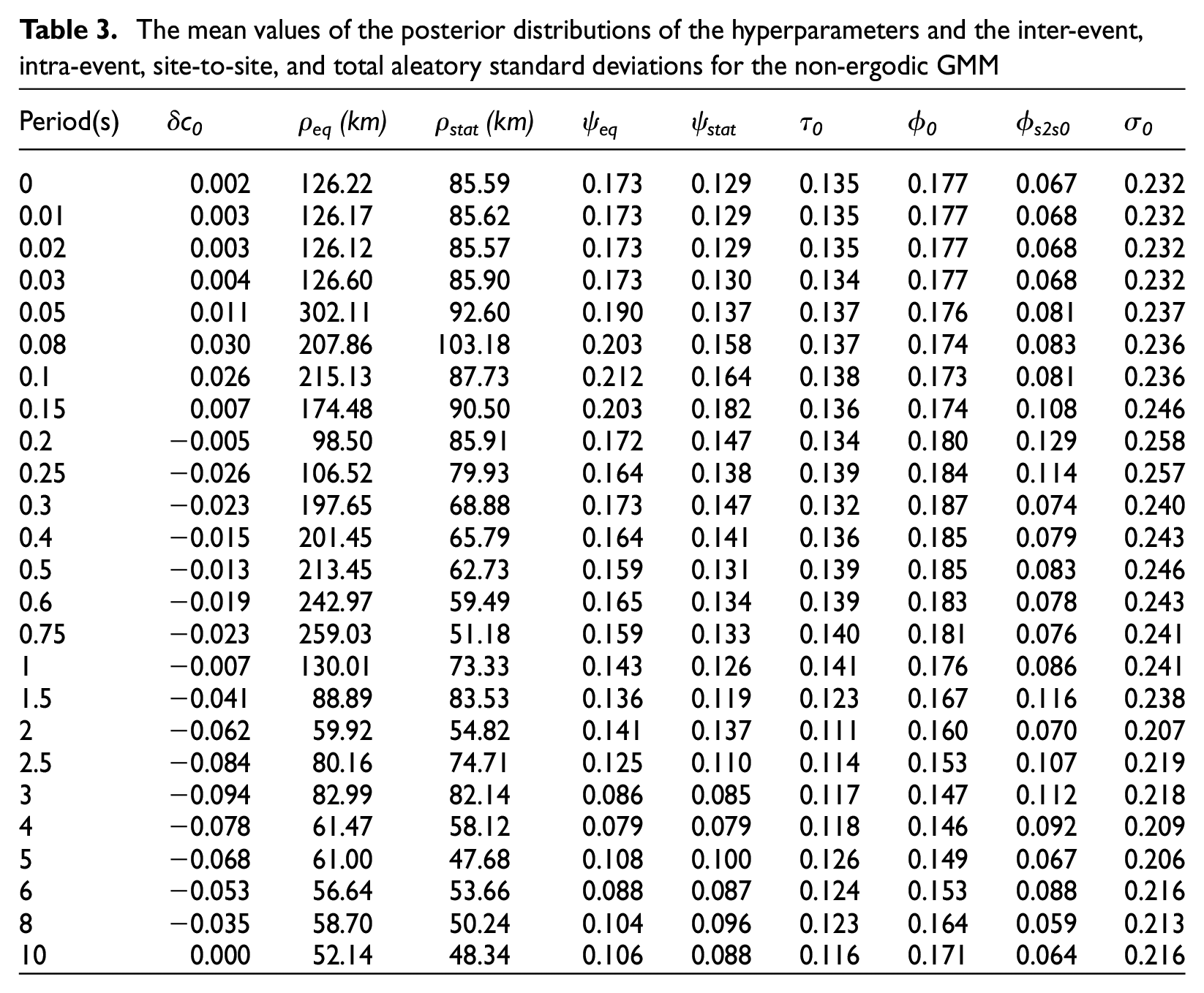
Figure 21 shows maps of the mean and SD of the spatially varying site effects (δcstat) for PGA and spectral accelerations at T = 0.5, 1.0, and 8.0 s. Figure 21a, c, e, and g show that the positive and negative values of the spatially varying site effects change as the period changes. The negative values of spatially varying site effects are distributed mainly near the coast at short periods and transition to be distributed near the trench as the period increases. Conversely, the positive values of spatially varying site effects are distributed mainly near the trench at short periods and transition to be distributed near the coast as the period increases. Figure 21b, d, f, and h shows the SDs of the spatially varying site effects, which is similar to the spatially varying source effects. In regions without station distribution, the site effects have near-zero means and large SDs. The spatial pattern exhibited by the spatially varying site effects indicates that the spatial correlation length does not change much in different periods. The hyperparameter ρ that control the range of spatial correlation length of spatial varying terms is shown in Table 3. The reason why the spatial correlation length of the spatially varying site effects remain relatively stable may be attributed to many factors, such as station density (ie., the 150 offshore stations are uniformly distributed near the Japan Trench), consistency of site conditions and geological stability (ie., each station maintains a stable site condition at a fixed location for different periods).
These non-zero means of spatially varying source and site effect coefficients represent source and site characteristics that cannot be captured by the ergodic backbone GMM. However, these systematic and repeatable source and site effects can be constrained using the ground motion records in the non-ergodic GMM.
Figure 22 shows the estimated mean and SD of the site-specific adjustment term δS2S0 for PGA. The mean values of δS2S0 do not exhibit spatial correlation (i.e. the spatial correlation length of δS2S0 is zero, and there are no systematic positive or negative regions), indicating that spatially varying site effects δcstat correctly capture the spatial correlation component of the site effects.
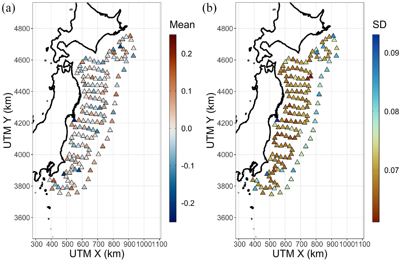
The estimated (a) mean and (b) standard deviation of the site-specific adjustment term δS2S0 for PGA.
The cell-specific attenuation coefficient
Figure 23 shows the mean and epistemic SD of the cell-specific anelastic attenuation coefficient ci of each cell for PGA and SaRotD50 (1 s). The cell-specific anelastic attenuation coefficients represent systematic and repeatable path effects. For cells without paths, the mean cell-specific anelastic attenuation coefficients ci are considered to be consistent with the anelastic attenuation coefficient k(T) of the ergodic backbone GMM. Furthermore, most of the cell-specific anelastic attenuation coefficients are consistent with the anelastic attenuation coefficient k(T) of the ergodic GMM. However, some cell-specific anelastic attenuation coefficients exhibit nonphysical behavior, with a small amount of positive cell-specific attenuation coefficients in the region. Figure 23c shows nonphysical behavior for SaRotD50 (1 s) in the region of buried stations due to the increased ground coupling of buried stations. Cells containing a large number of paths have smaller epistemic SDs, while cells containing fewer paths have larger epistemic SDs. The large epistemic SD implies that the current data set is insufficient to provide a good estimate of the cell-specific anelastic attenuation coefficient in this cell.
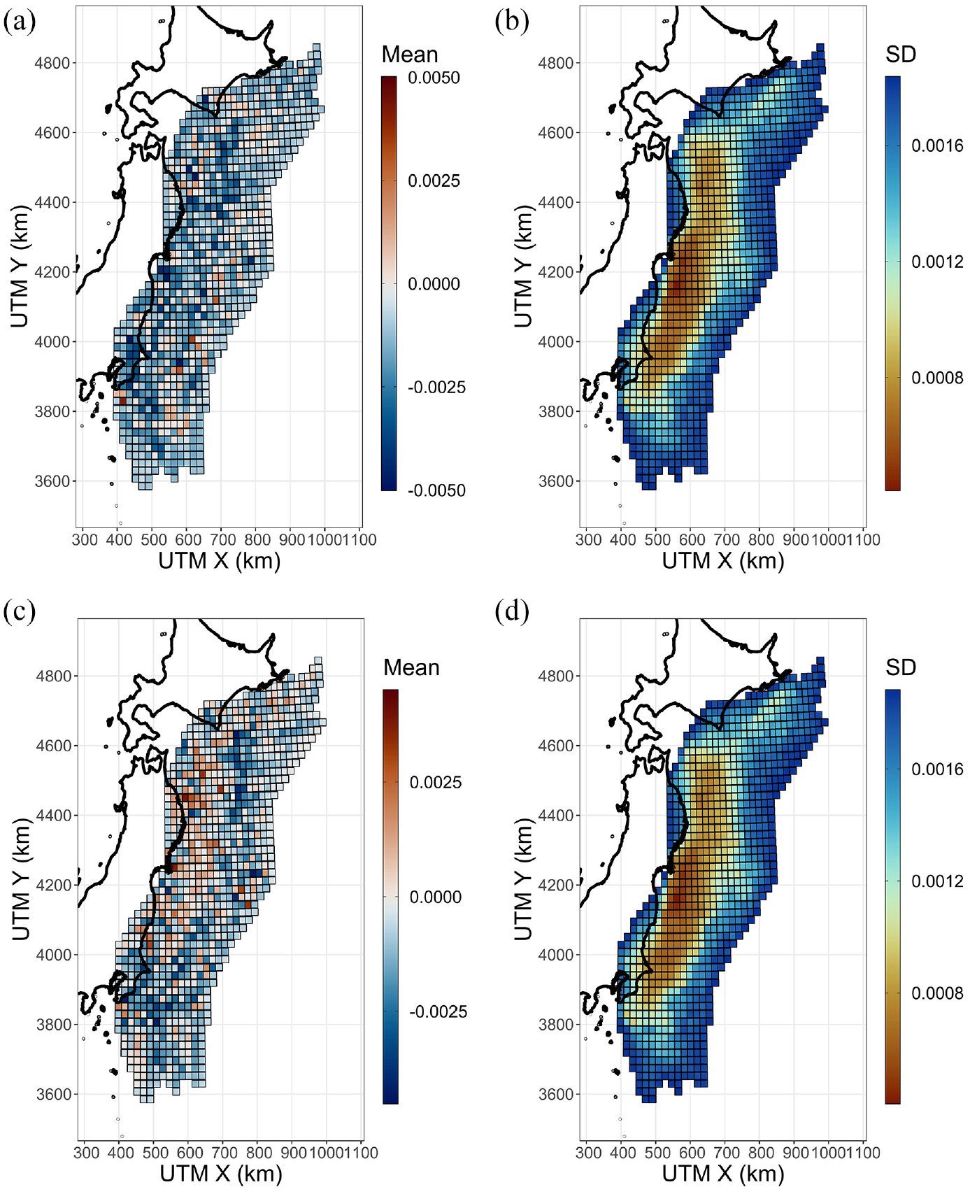
The mean anelastic attenuation coefficient and epistemic standard deviation of each cell estimated by the cell-specific anelastic attenuation method: (a) the mean cell-specific anelastic attenuation coefficients for PGA; (b) the epistemic standard deviations for PGA; (c) the mean cell-specific anelastic attenuation coefficients for SaRotD50 (1 s); and (d) the epistemic standard deviations for SaRotD50 (1 s).
Residuals and standard deviations
Figure 24 shows residual analysis of non-ergodic GMM with respect to moment magnitude (M), rupture distance (Rrup), thickness of sediment up to Vs = 1.4 km/s (D14), and water column for PGA and spectral accelerations at T = 0.5 and 1.0 s. Compared with Figure 9, the distribution of residuals with respect to each explanatory variable (ie., M, Rrup, D14, and water column) has less scattering and become more concentrated near zero. This is due to the fact that the non-ergodic GMM incorporates repeatable and systematic source, site, and path effects into the ergodic GMM, which makes the non-ergodic GMM have less epistemic uncertainty.
Residual analysis of non-ergodic GMM with respect to moment magnitude (M), rupture distance (Rrup), thickness of sediment up to Vs = 1.4 km/s (D14), and water column for PGA and spectral accelerations at T = 0.5 and 1.0 s. (a1)–(a3) the inter-event residuals versus moment magnitude; (b1)–(b3) the intra-event residuals versus moment magnitude; (c1)–(c4) the intra-event residuals versus rupture distance; (d1)–(d3) the intra-event residuals versus thickness of sediment up to Vs = 1.4 km/s; (e1)–(e3) the intra-event residuals versus water column. Orange circles and green error bars represent the mean and standard deviation of the residuals, respectively.
Figure 25 shows the inter-event, intra-event, and total aleatory SD terms of the ergodic and non-ergodic GMM for each period. The non-ergodic GMM exhibits a significant reduction in aleatory variability, with the values of the total aleatory SDs reduced by about 22%–39%. This reduced aleatory variability is important for explaining the epistemic uncertainty in the non-ergodic terms and for performing non-ergodic PSHA. The mean values of the posterior distributions of the hyperparameters, as well as the inter-event, intra-event, site-to-site, and total aleatory SDs for the non-ergodic GMM, are listed in Table 3 for periods from 0 to 10 s. The hyperparameters of spatially varying source effects vary greatly, ranging from 52 to 302 km in different periods; while the hyperparameters of spatially varying site effects vary slightly, ranging from 47 to 103 km.
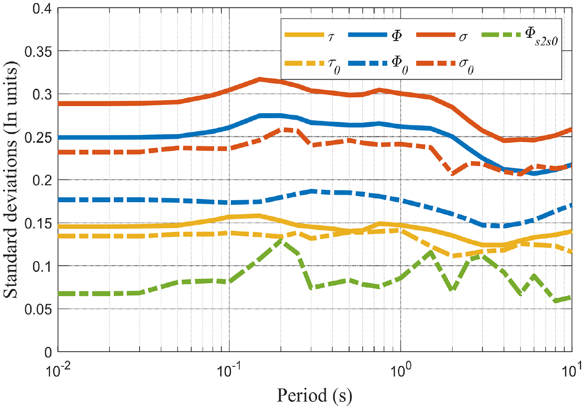
The inter-event, intra-event, and total aleatory standard deviation terms of ergodic backbone and non-ergodic GMM for each period.
Conclusion and discussion
An offshore ergodic backbone GMM for subduction earthquakes in the Japan Trench region was developed in this study, and its functional form was implemented by modifying the GMM of Si et al. (2022). Site amplification was investigated by classifying S-net stations into four site categories using horizontal-to-vertical response spectral ratio (HVRSR). The amplitudes and shapes of the mean HVRSR of four site categories were significantly different, especially for unburied stations. The offshore ergodic GMM can accurately capture the observed offshore ground motion in terms of distance scaling for different subduction earthquake scenarios. It is applicable for subduction earthquake scenarios in the Japan Trench area with moment magnitudes ranging from 4.0 to 7.4 and rupture distances ranging from 10 to 300 km. In addition, we compared the offshore ergodic GMM with NGA-Sub GMMs and some GMMs from Japan in terms of attenuation curves and response spectra. The results showed that offshore GMMs are significantly different from onshore GMMs for subduction earthquakes, especially in the long-period and unburied states, which highlights the impracticality of directly applying onshore GMMs to offshore regions. The large differences between onshore and offshore GMMs may be related to the deployment method of the seafloor stations, the degree of coupling between the stations and the seafloor, the topography of the seafloor, the thickness of the seafloor sediment, and the depth of seawater. The significant differences between buried and unburied stations indicated that the unburied stations are more susceptible to the influence of complex seafloor environments. Therefore, it is necessary to develop reasonable prediction models for offshore ground motion, particularly for subduction earthquakes that can cause significant damage.
The non-ergodic GMM for subduction earthquakes was developed based on the offshore ergodic backbone GMM. In the non-ergodic GMM, the systematic and repeatable source and site effects were captured by the spatially varying coefficients represented by Gaussian processes; the systematic and repeatable path effects were captured by cell-specific anelastic attenuation proposed by Dawood and Rodriguez-Marek (2013), calculated with the Cohen–Sutherland computer graphics algorithm. The spatial pattern exhibited by the spatial varying source effects varied slight for different periods. The positive values of the spatially varying source effects were mainly concentrated on the side near the coast, while the negative values were mainly scattered on the offshore side. However, the spatial pattern exhibited by the spatial varying site effects varied continuously with the period. The negative values of site effects were mainly distributed near the coast in short periods, transitioning to be distributed near the trench in long periods. Conversely, the positive values of site effects were mainly distributed near the trench in short periods, transitioning to be distributed near the coast in long periods. The spatial varying source and site effects had near-zero means and large epistemic SDs for regions without epicenter and station distributions, implying that there are not enough data to constrain the systematic and repeatable source and site effects. The mean anelastic attenuation coefficient and epistemic SD of each cell calculated by Bayesian inference with INLA can represent systematic and repeatable path effects. Cells containing a small number of paths had larger epistemic SD. The epistemic uncertainty of spatially varying effects is consistent with intuitive data availability. This implies that the epistemic uncertainty of estimated spatially varying effects is greater for regions without sufficient data.
Compared to the residuals of ergodic GMM, the distribution of residuals of non-ergodic GMM with respect to each explanatory variable had less scattering and was more concentrated around zero. This is because the non-ergodic GMM incorporates systematic and repeatable source, path and site effects into GMM. In addition, the values of the total aleatory SDs of non-ergodic GMM were reduced by about 22%–39%. The non-ergodic GMM developed in this study can better capture the aleatory variability and epistemic uncertainty of ground motion in the Japan trench region. Such aleatory variability and epistemic uncertainty should be incorporated into PSHA calculations because a small variation in SDs can lead to an underestimation of seismic risk. These results can provide a basis for rational seismic design and seismic risk assessment of marine engineering in offshore subduction zone, as well as the prediction of ground motions for EEW and seismic demand analysis of offshore facilities in the Japan Trench region.
Footnotes
Acknowledgements
The authors would also like to thank the National Research Institute for Earth Science and Disaster Resilience (NIED) and the Full Range Seismograph Network of Japan (F-net)) for providing the strong ground motion data. They specially thank the anonymous reviewers, as well as the editor and associate editor for their precious review comments. Plots were made using the R package ggplot2 (Wickham, 2016). The geophysical maps were made using Generic Mapping Tools (GMT).
Declaration of conflicting interests
The author(s) declared no potential conflicts of interest with respect to the research, authorship, and/or publication of this article.
Funding
The author(s) disclosed receipt of the following financial support for the research, authorship, and/or publication of this article: This research was supported by the Study on Failure Mechanism and Seismic Design Theory of Step-back Building Structures in Mountainous Regions (grant no. 51638002) and the Study on Seismic Performance of Ceramsite Concrete Filled Steel Plate Composite Shear Wall Structure (grant no. 52278484).
Data and Resources
The S-net data were downloaded from the following website address: (https://hinetwww11.bosai.go.jp/auth/download/cont/?LANG=en). The information regarding earthquake events is drawn from Japan Meteorological Agency (JMA) catalogs (https://www.fnet.bosai.go.jp/event/search.php?LANG=en). The thickness of the sediment layer to Vs 1.4 km/s for S-net stations was downloaded from the website (![]() ), which is operated by the Japan Seismic Hazard Information Station (J-SHIS).
), which is operated by the Japan Seismic Hazard Information Station (J-SHIS).