
Abstract
Site amplification maps are mostly proxy-based. Often due to the absence of in-situ data at the regional or local scale, a high level of confidence cannot be assigned to the site amplifications. It has often been observed that the in-situ amplifications differ from proxy-based estimates. So, whenever new in-situ data are made available, it is necessary to update the proxy-based estimates. Bayesian frameworks are recently gaining attention as model updating schemes. This study proposes a Bayesian scheme for updating proxy-based maps with in-situ data. This scheme is based on uncertainty projected mapping (UPM), where the significance of local in-situ data variability determines the posterior estimates. The study area is in Osaka, Japan, where discrepancies in proxy-based estimates and observed ground motions were documented during the 2018 Northern Osaka earthquake. Dense borehole data from the Kansai Geo-informatics Network are available in this area. Peak ground velocity (PGV) site amplification evaluations from this dense borehole network are used as likelihoods to update the prior proxy-based Japan seismic hazard information system (J-SHIS) site amplification map. As a result, the posterior map shows updated site amplification estimates which better represent the in-situ data. The updated site amplification map is then used to investigate the role of site amplification in explaining the building damage during the 2018 Northern Osaka earthquake.
Introduction
In seismic hazard and risk assessment, the focus is gradually shifting from the national to the regional scale. An essential prerequisite for accurate risk assessment at regional and local scales is a precise site amplification map at these scales, which demands detailed knowledge of geotechnical properties at the site, such as borehole data and PS logging. However, acquiring in-situ knowledge of geotechnical properties is highly cost-intensive. Hence, proxy parameters are often used to estimate site amplification.
One widely used proxy parameter is Vs30, the shear wave velocity in the top 30 m of soil. Borcherdt (1994) introduced a relationship between site amplification and Vs30 with soil data sets from the United States. Similarly, Fujimoto and Midorikawa (2006) established a relationship between Vs30 and site amplification in Japan. Estimating Vs30 demands detailed knowledge of geotechnical properties, for which various proxy parameters have been developed. The topographic slope from digital elevation models (DEMs) is frequently used as a reliable proxy for Vs30 (Allen and Wald, 2009; Wald and Allen, 2007). Matsuoka et al. (2006) proposed using geomorphic classifications as a proxy for Vs30. There is extensive literature on the estimation of site amplification via Vs30, which itself is based on proxy parameters like engineering geology and topography (Heath et al., 2020; Kwok et al., 2018; Park and Elrick, 1998; Thompson et al., 2014; Thompson and Wald, 2012; Vilanova et al.,2018; Wills et al., 2000; Wills and Silva, 1998).
However, proxy parameters do not always accurately represent site amplification and their limitations have been reported in the literature. Castellaro et al. (2008) question the significance of the correlation between site amplification and Vs30 even in the original dataset of Borcherdt (1994). Weatherill et al. (2020) demonstrate the limitations of using topographic slope as a proxy for Vs30. During the 2018 Mw 5.6 Northern Osaka earthquake in Japan, the observed ground shaking in the epicentral area significantly deviated from the proxy-based site amplification estimations of Japan seismic hazard information system’s (J-SHIS) (Asano et al., 2021; Fujiwara et al., 2006a, 2006b; Kiyono et al., 2021). This map is a peak ground velocity (PGV) site amplification map based on Vs30 values derived from engineering geomorphic classifications. Thus, there is a need to update proxy-based maps as and when in-situ data becomes available.
In recent years, there has been a global effort by all concerned stakeholders (government, state, academic institutions, and private organizations) to expand the database of in-situ data and improve the understanding of the seismic site effects. In addition to borehole data and PS logging, Vs30 measurements from ambient vibration studies are now considered a reliable source of in-situ information. In the United States, the United States Geological Survey (USGS) has published a map with measured Vs30 values from borehole data and ambient vibration studies funded by USGS and other governmental agencies (McPhillips et al., 2020). In Europe, a publicly available measured Vs30 values database was published as part of the European Seismic Risk Model (ESRM20; Weatherill et al., 2022). In Japan, in addition to the borehole data available at the strong motion seismograph network of K-NET and KiK-net (National Research Institute for Earth Science and Disaster Resilience, 2019), the Ministry of Land, Infrastructure, Transport and Tourism (MLIT), the Public Works Research Institute (PWRI) and the Port and Airport Research Institute (PARI) also maintains a public database of borehole data compiled from different projects all over Japan (Kunijiban, 2008).
Bayesian frameworks are recently gaining attention as model updating schemes (De Risi et al., 2021; Foster et al., 2019; Noh et al., 2020; Powers et al., 2021; Silva et al., 2020). The main idea behind the Bayesian framework lies in the Bayes theorem, which proposes an equation to update existing knowledge based on the arrival of new information (Bayes, 1763). In a Bayesian framework, three distributions should be understood. The first one is the prior distribution or prior, which is the existing knowledge or the probability before the new information is considered. The second one is the likelihood distribution or likelihood, which is the probability of the new information. And the third one is the posterior distribution or posterior, which is the updated probability after the new information is considered. The mean of this posterior distribution is usually referred to as the posterior estimate. A Bayesian framework, thus, allows updating the existing knowledge (prior) with new information (likelihood), and the updated knowledge is termed the posterior.
The advantage of the Bayesian framework lies in its capability to handle the uncertainties in the prior and the likelihood systematically. For example, in the research problem of updating proxy-based site amplification maps with in-situ data, uncertainties will arise from the site-specific variability and spatial density variability of the in-situ data. Uncertainty projected mapping (UPM), introduced by Chakraborty and Goto (2018), which considers site-specific uncertainty and between-site uncertainty, has the potential to incorporate these uncertainties in in-situ data.
This study proposes a Bayesian updating scheme based on the framework of UPM. In UPM, the posterior estimates are determined by the significance of local in-situ data variability. The significance is determined by the extent of data overlap between neighboring meshes in a local area. The higher the extent of data overlaps, the lower the significance of the in-situ data variability. Areas with a significantly high local variation result in a non-uniform posterior estimate, whereas those with significantly low local variation result in uniform posterior estimates. Thus, the significance of the local in-situ data variation is reflected in the uniformity of the posterior estimates. The Bayesian framework of UPM allows updating a proxy-based site amplification map (prior) with the new in-situ data (likelihood).
UPM considers the statistical significance of differences in neighborhood values in determining a variable’s value at a site. This technique is very different from the conventional mapping tools, for example, Kriging (Matheron, 1963), in its treatment of uncertainties. In Kriging, averaged observation values are assigned to the sites, and the information on the site-specific uncertainty is lost. Two sites might be different only because of their difference in average values. But what if the data distribution is overlapping? Is the difference between the two sites statistically significant? The conventional mapping tools do not consider this. In previous studies, UPM has successfully separated sites with no significant overlap in the data distributions and unified sites with significant overlap in data distributions (Chakraborty and Goto, 2018, 2020). In UPM, the decision-making is based on all the available data, whereas Kriging uses a single averaged value. However, this property of UPM to make decision-making based on the statistical significance of neighborhood differences works best when the number of observations is low. As the number of observations increases, the UPM converges with the Kriging (Chakraborty and Goto, 2020).
Our study area is near the epicentral region of the 2018 Northern Osaka earthquake in Osaka, Japan. In this area, the observed building damage distribution did not agree with the estimations of the proxy-based J-SHIS site amplification map. Studies show that the damage distribution during an earthquake depends not only on the site amplification but also on factors such as the source directivity effect, age of buildings, and so on. However, it is essential to confirm or negate the role of site amplification in the observed damage distribution.
In the study area, dense borehole data from the Kansai Geo-informatics Network is available. Recent studies have highlighted the limitations of simulated site amplification. Zhu et al. (2022) elaborate on the higher accuracy of empirical amplifications over simulated site amplifications. For KiK-net stations in Japan, where observation records at surface and borehole depth are available, methodologies for obtaining empirical amplifications have been proposed (Kotha et al., 2018; Régnier et al., 2013). However, the availability of observation records is a prerequisite for calculating the empirical amplifications. Also, for using the empirical amplifications in the UPM framework, enough seismic records are required because site-specific variation needs to be addressed. At the dense borehole locations, earthquake observation records are not available for calculating the empirical amplifications in the UPM framework. So, the authors employed simulated site amplifications in this study. Site amplifications were evaluated using one-dimensional (1D) seismic ground response analysis (Yoshida, 2015). The evaluated site amplifications are PGV-based, as the objective is to update the proxy-based J-SHIS site amplification map, which is also PGV-based. In this study, the PGV site amplifications evaluated at the borehole locations are called “in-situ site amplifications.” In Bayesian terminology, these in-situ site amplifications are the likelihoods. These are used to update the prior, which in this study is the proxy-based J-SHIS site amplification map (Hereafter termed “proxy-based J-SHIS map”) in Osaka, Japan.
The posterior or the updated site amplification map was then used to investigate the role of site amplification in explaining the building damage during the 2018 Northern Osaka earthquake.
Study area
Figure 1a shows the location of the study area on the map of Japan. The study area expands over the Ibaraki and Takatsuki cities of Osaka, Japan. This area is near the epicenter of the 2018 Northern Osaka earthquake and covers many building damage areas observed during the earthquake.
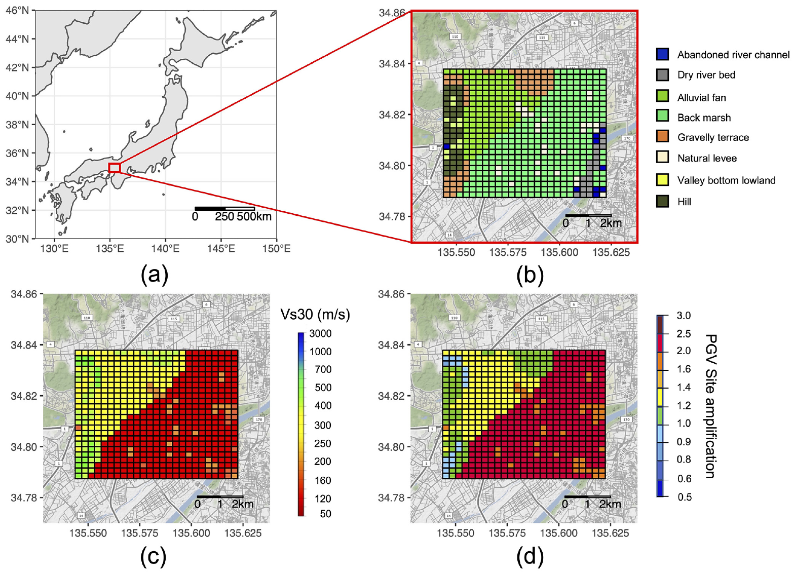
(a) The study area in Osaka (in red rectangle) is shown on the map of Japan. J-SHIS’s (b) engineering geomorphology map, (c) Vs30 map, and (d) PGV-based site amplification map. The mesh size is 250 m × 250 m.
In this study, the authors used the block-level building damage map prepared by Asano et al. (2021) as a reference. The resolution of this damage map is at Cho-Cho-Moku (in Japanese), the smallest unit of geographic area at the sub-municipality level in Japan. The damage map is not pixelated or rasterized. The idea of Cho-Cho-Moku is similar to the usage of “block” in a US city. In Japan, after a post-earthquake inspection, government authorities issue house owners a building damage certificate, proof of the extent to which a building was damaged. In their study, Asano et al. (2021) quantified damage as the number of building damage certificates received per building in a block. The block with a higher building damage certificate per building has higher damage and vice versa. This map is shown in Figure 18a in the “Discussions” section, which forms the basis of all damage-related discussions in this paper. Asano et al. (2021) concluded that most of the building damage did not align with the estimations of the proxy-based J-SHIS map. The findings by Kiyono et al. (2021) also supported this conclusion.
Figure 1b to d show the J-SHIS’s engineering geomorphology, Vs30, and site amplification maps in the study area. The mesh-size is 250 m × 250 m. The site amplification map is derived from the engineering geomorphology and the Vs30 map. The spatial resolution of the engineering geomorphology map is 250 m throughout Japan. In the first step, linear regression generates the Vs30 map from the engineering geomorphology map (Wakamatsu and Matsuoka, 2013). In the second step, the site amplification map is calculated from the Vs30 map using Fujimoto and Midorikawa (2006).
Dense borehole data from the Kansai Geo-informatics Network is available in the study area. Figure 2 shows the locations of around 3800 boreholes in and around the study area (marked by a red rectangle). The borehole data provide the no. of blows (N-values) of the standard penetration test (SPT) and soil classification. Figure 3 shows the distribution of the borehole depth of 3800 boreholes as a histogram (Boreholes with no SPT N-values are omitted). About 485 out of 3800 borehole locations are inside the study area. These data are not included in the proxy-based J-SHIS map but can potentially improve the site amplification in the study area. The updated site amplifications can help discuss the damage distribution of the 2018 Northern Osaka earthquake. As the objective of this study is to update the proxy-based J-SHIS map, the same mesh size (250 m × 250 m) was used in preparing the updated map.
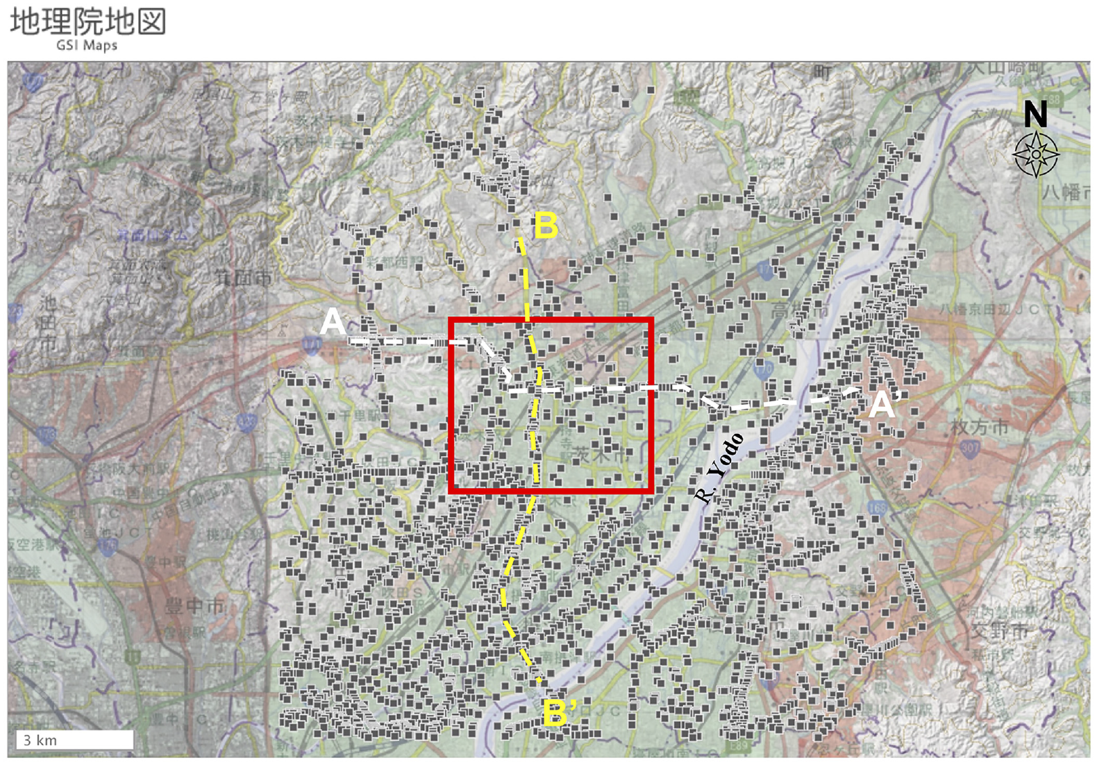
The small black squares represent the borehole locations from Kansai Geoinformatics Network. A-A’ and B-B’ are the main sections along which the cross-section of soil structure is investigated.
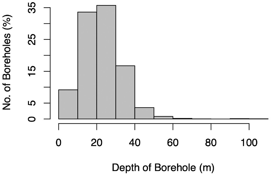
Histogram of the depth of borehole at the 3800 locations. The boreholes with no information on SPT N-value have been omitted.
Method
A Bayesian updating scheme is ideal for updating the proxy-based J-SHIS map in Osaka, Japan, with additional information from borehole data. In a Bayesian updating scheme, the prior is the existing knowledge, and the likelihood is the additional or new information. The updated knowledge, known as the posterior, is estimated using Bayesian inference.
The different steps of the method employed in this study to update the proxy-based J-SHIS map are summarized in Figure 4. At first, mesh-wise priors and likelihood distributions are evaluated at each 250 m × 250 m mesh of the study area. The mesh-wise prior and likelihood distributions are quantified using the mesh-specific mean (
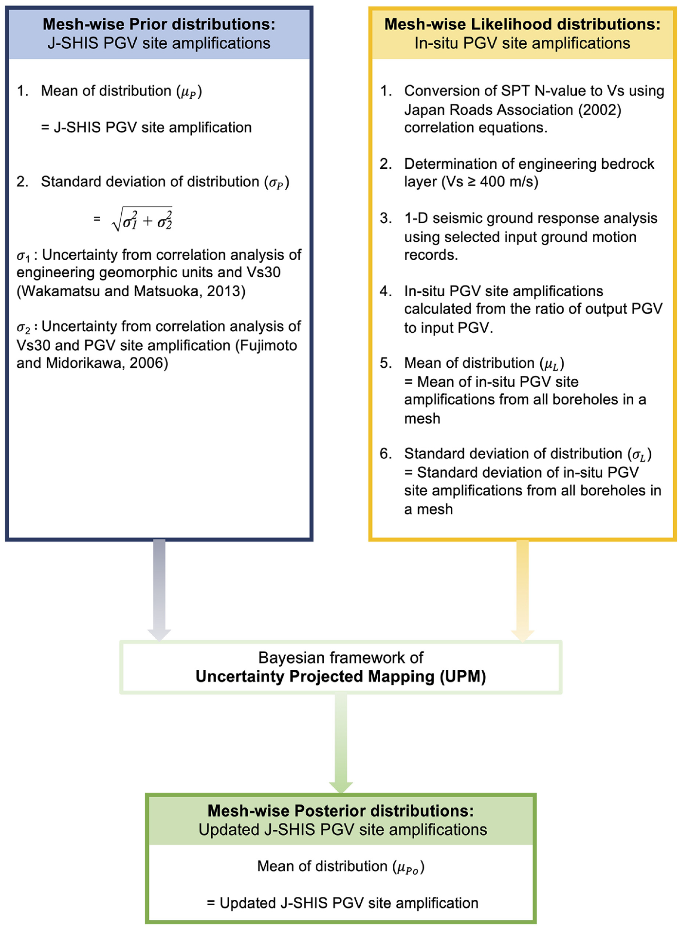
Graphical representation of the method employed in this study to update the J-SHIS PGV-based site amplifications.
The Bayesian framework of UPM incorporates the

In this article, the UPM methodology introduced by Chakraborty and Goto (2018) is called the Original UPM. Equation 2 shows the Bayesian framework of the Original UPM:
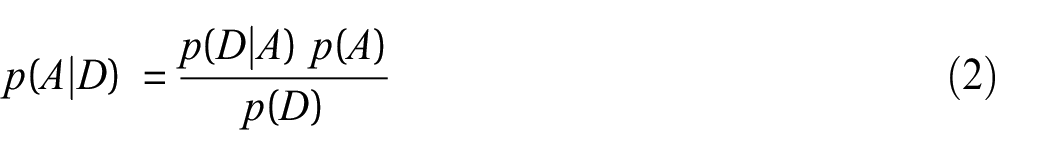
where
In the proposed Bayesian updating scheme, the proxy-based J-SHIS site amplifications are adopted as the prior information of the Bayesian inference. Using Bayes’ theorem, the updated site amplifications
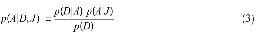
J refers to the information from the proxy-based J-SHIS map; thus,
Priors and likelihoods of site amplifications
Prior site amplifications: proxy-based J-SHIS site amplifications
The prior distribution of the site amplification is evaluated at each 250 m × 250 m mesh of the proxy-based J-SHIS map. Researchers generally model site amplification as log-normally distributed (Bahrampouri et al., 2019a; Bazzurro and Cornell, 2004; Li and Assimaki, 2010; Rathje et al., 2010). However, this assumption may not always be correct. Recently, Bahrampouri et al. (2019b) recommended using skew-normal distribution for site amplification, especially at high intensities. In this study, however, for ease of modeling, we follow the general assumption and model the site amplifications as log-normally distributed. Thus, the prior is assumed to be log-normally distributed.
The prior distribution’s mean (
The standard deviation of the prior distribution (
Figure 5 shows the mean (
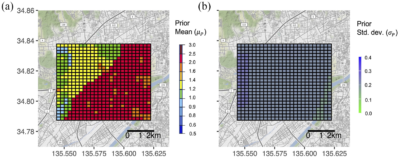
(a) Mean and (b) standard deviation for the prior site amplification (J-SHIS). The mesh size is 250 m × 250 m.
Likelihoods of site amplifications: in-situ PGV site amplifications
In-situ site amplifications estimated using 1D seismic ground response analysis (Yoshida, 2015) constitute the likelihood distribution. The site amplification variability at each borehole location results from the variability of the input ground motions used in the analysis. PGV amplifications determine the proxy-based J-SHIS site amplifications. Similarly, the in-situ site amplifications are defined as the ratio of the PGV of input earthquake motion at the engineering bedrock to the PGV of output earthquake motion at the ground surface at each borehole location.
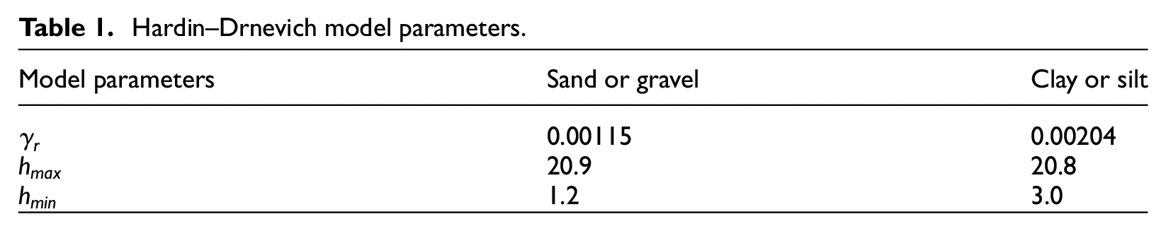
In this study, 1D seismic ground response analysis is performed using the computer program of DYNamic response analysis of level ground by the EQuivalent linear method (DYNEQ; Yoshida, 2015; Yoshida et al., 2002). SHAKE was selected (Schnabel, 1972) as the dynamic ground response analysis method. In addition, non-linear modeling of soil was employed using the Hardin–Drnevich (H-D) model, with the model parameters listed in Table 1 (Hardin and Drnevich, 1972a, 1972b). The parameters of the H-D model are based on a geological model of the Osaka sedimentary basin. Goto et al. (2018) published G/G0-γ and h-γ curves based on cyclic shear deformation tests on soil obtained from 280 borehole locations of the Osaka sedimentary basin. These curves were then fitted with the H-D, Ramberg–Osgood, and Double Hyperbolic models. Out of these three models, the H-D model has the best fit. So, in this study, the H-D model parameters of Goto et al. (2018) were used as target curves for the H-D model. The H-D model directly sets up the h-γ relation. No Masing rule is used in the equivalent linear analysis. Htun et al. (2019) also used the model parameters published by Goto et al. (2018).
Hardin–Drnevich model parameters.
The borehole data from the Kansai Geoinformatics group provides the SPT N-values and soil classification. Information from both was utilized to differentiate the sand/gravel and clay/silt group. Also, there was no borehole data that could help distinguish different rock types in the boreholes. Although Osaka sedimentary basin area has been extensively studied, our study area is relatively less investigated as it is near the edge of the basin. Ito et al. (2018) did an extensive borehole data analysis with the borehole data from the Kansai Geoinformatics network. However, our study area was barely touched, and no other borehole data (in addition to N and soil classification) were available to differentiate the different sand/gravel and clay/silt groups. Asano et al. (2017) studied the Osaka sedimentary basin with ambient noise cross-correlation functions. They hinted at a shallower seismic bedrock (200∼800 m) in our study area, which is almost at the edge of their focus area.
The shear-wave velocity (


For sand and gravel, if SPT N-value ≥ 50, the
We assume the uncertainty of the Vs estimates from the Japan Road Association (2002) formula to be low because these correlations have been widely validated over time through many applications in Japan and elsewhere in the world (Anbazhagan and Sitharam, 2008; Chatterjee and Choudhury, 2013; Mhaske and Choudhury, 2011).
As for the density, 2000 kg/m3 is assigned for sand and gravel, and 1800 kg/m3 for clay and silt.
In 1D seismic ground response analysis, it is necessary to determine a soil layer that can be treated as the engineering bedrock. In the design specifications of Japan, the engineering bedrock is defined by the SPT N-value and the corresponding
In the United States, the reference Vs for engineering bedrock is 760 m/s. In Japan, the reference Vs for engineering bedrock is 400 m/s. An exception is the case of nuclear power plant design, where Vs = 700 m/s is used as the engineering bedrock. The site amplification in the J-SHIS map has been calculated as the amplified ratio from the engineering bedrock of Vs = 400 m/s to the ground surface. As the objective of this study is to update the J-SHIS map, we used the same Vs = 400 m/s for the engineering bedrock.
Although there might be concerns about the detrimental effect on succeeding studies, especially related to liquefaction hazard characterizations, several liquefaction-related studies have been published using Vs = 400 m/s or higher for the engineering bedrock or elastic half-space. Pender et al. (2016) used Vs = 400 m/s for the elastic half-space to investigate the effect of permeability on the cyclic generation and dissipation of pore pressures in saturated gravel layers in Christchurch, New Zealand. Fukutake and Jang (2013) and Nakai et al. (2016) used a Vs of 430 m/s and 400 m/s for liquefaction potential studies in Urayasu, Japan. Mase et al. (2022) used Vs = 400 m/s as elastic half-space for liquefaction analysis in Osaka, Japan.
In Japan, the engineering bedrock is so defined that the predominant period is a little longer than the structure of interest. For buildings with long natural periods (super high-rise or base-isolated buildings), amplifications from the seismic bedrock or an engineering bedrock with a higher threshold are recommended. However, for most cases, Vs = 400 m/s works well. Régnier et at. (2014) observe that most seismic stations in Japan are located on thin sedimentary sites. Sites with high Vs contrast close to the surface might trigger non-linear behavior at low input motion PGA values. This observation might also be why 400 m/s is chosen as a threshold in Japan.
Yoshida (2015) elaborates on the effect of layers below engineering bedrock (Vs = 400 m/s). A 380-m deep soil profile with PS logging data in Japan is used as an example. The soil layer at 50 m depth with Vs = 379 m/s is set as the engineering bedrock layer. The seismic bedrock is a layer with Vs = 3000 m/s. Different cases are created where the thickness and Vs of the intermediate layer between the engineering bedrock and the seismic bedrock are varied. The thickness varies from 5 to 100 m, and the Vs varies from 200 to 700 m/s. The results show that the depth-wise variation of maximum acceleration, maximum stress, and maximum strain above the engineering bedrock are almost identical and indistinguishable in all the cases. The behavior of the subsurface layers is not significantly affected by the velocity structure below the engineering bedrock. Thus, Vs = 400 m/s is sufficient as a boundary condition as the behavior of the surface layers is independent of the behavior below the engineering bedrock.
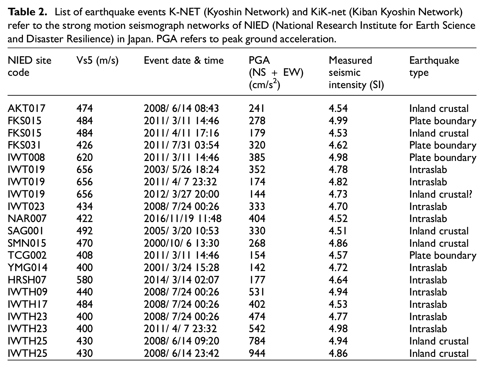
As for the input ground motions, ground motion records observed at stiff soil sites, which can be treated as engineering bedrock, are used. The stiff soil sites are selected from K-NET and KiK-net stations with the criterion that the shear-wave velocity in the top 5 m (Vs5) lies in the range of 400–700 m/s. The stiff soil sites selected under this criterion correspond to the soil stiffness of the defined engineering bedrock in this study. Among the earthquake records obtained at these stations, the records with a measured seismic intensity between 4.5 and 5.0 in the Japan Meteorological Agency (JMA) seismic intensity scale is selected. Based on the abovementioned criteria, 21 records are selected (Table 2). The horizontal components (NS and EW) are used as input ground motions from each of these records, except the EW component of the last earthquake event, as the data had some technical issues. In total, 41 input earthquake ground motions are adopted.
List of earthquake events K-NET (Kyoshin Network) and KiK-net (Kiban Kyoshin Network) refer to the strong motion seismograph networks of NIED (National Research Institute for Earth Science and Disaster Resilience) in Japan. PGA refers to peak ground acceleration.
Once the soil model, engineering bedrock, and input ground motions are selected, 1D seismic ground response analysis is performed, and PGV site amplifications are calculated at each borehole location. The evaluated in-situ PGV site amplifications are then assigned to the respective standard area mesh of 250 m × 250 m, identical to the mesh size of the proxy-based J-SHIS map, for the evaluation of mean (
Depending on the location of the borehole, the number of sites in each mesh will vary considerably. However, no under-sampling or over-sampling techniques have been employed in this study.
The posterior distribution in Bayesian-based UPM is estimated using MCMC simulations. The advantage of MCMC estimation is that, like bootstrapping, it provides mean and standard deviation values for an accurate representation of finite sample uncertainty.
However, the bottleneck of this study was the determination of the engineering bedrock layer. In the study area, deciding on a single layer as the engineering bedrock layer was almost impossible, so soil zonation was employed. The following section discusses the distribution of the engineering bedrock in the study area.
Distribution of the engineering bedrock
The knowledge of engineering bedrock is essential to calculate the in-situ site amplifications using 1D seismic response analysis. The determination of engineering bedrock depends on the confirmation of spatial continuity of a stiff candidate layer. In the study area, the spatial distribution of the engineering bedrock is investigated based on the available borehole data.
The general soil structure in the study area is discussed using two main sections, A and B, which include borehole data from outside the study area (Figure 2). A and B are selected as the main sections because there is a high density of borehole data. The color legends of the soil columns are summarized in Figure 6.
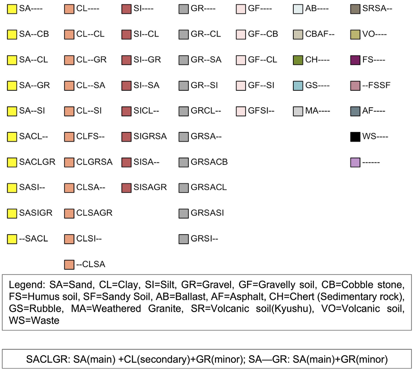
Color legend for different soil types in the borehole data.
It is observed that section A-A’, to some extent, follows the decrease in basin elevation from the mountain area to River Yodo. The cross-section of soil structure along section A-A’, as shown in Figure 7, shows a gravel layer that continues almost across the whole section. Above the gravel layer are sediments whose depth increases from east to west and reaches a maximum depth near River Yodo. In the middle of the section, the sediments are clay dominated; however, as one moves closer to the riverbed, the sand dominance increases. In Figure 7, the SPT-N ≥ 50 soil layers are highlighted with black boxes. It is observed that the gravel layer on the eastern side between locations 4 and 6 can be assumed to be the engineering bedrock. However, the shallow gravel layer on the western side cannot be treated as the engineering bedrock as it barely reaches SPT-N ≥ 50. Also, toward the middle of section A-A’ (near location 4), the available borehole data are insufficient to confirm if the same gravel layer connects from west to east. Thus, based on the available borehole data in section A-A’, it seems difficult to assign a standard gravel layer as the unique engineering bedrock for the whole study area.
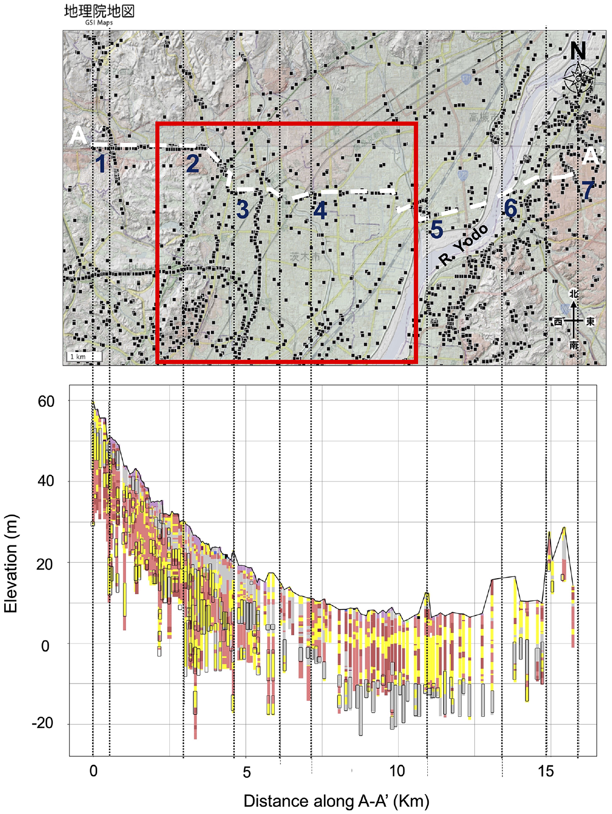
Cross-section of soil structure along section A-A’.
In section B-B’ (as shown in Figure 8), the borehole data between locations 3 and 4 is along an old river channel, which explains the gravel layer being so close to the surface. Upon superimposing with SPT-N ≥ 50 soil layers (black boxes), it is seen that this gravel layer could be considered the engineering bedrock. However, around location 4, the available data is insufficient to decide on the continuity of the engineering bedrock. As observed in section A-A, the sand dominance increases here as the borehole location moves closer to a riverbed.
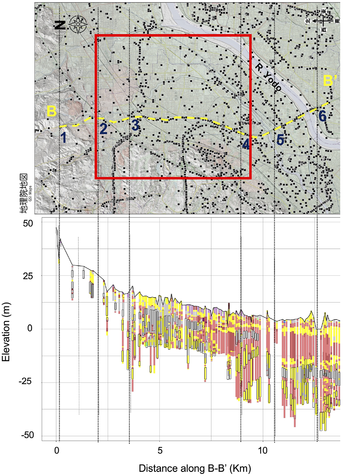
Cross-section of soil structure along section B-B’.
Thus, based on the general soil structure in the study area using sections A-A’ and B-B’, it is observed that assigning a standard gravel layer as the unique engineering bedrock for the entire study area is difficult.
As it is difficult to assign a standard layer as the engineering bedrock in the study area, in the next step, the soil structure in the study area is classified into certain zones using the findings along sections A-A’ and B-B’, combined with the borehole data outside the main sections. The authors would like to add that the zonation of the study area for engineering bedrock somewhat depends on the engineering judgment. This zonation aims to make the best use of the available information on soil structure in the study area to make engineering decisions and summarize the information to be usable for the study.
As shown in Figure 9, the zonation is based on the soil type. The yellow, red, and gray zones represent the sand-dominant, clay-dominant, and gravel-dominant soil, respectively. The orange zone represents the soil where it is difficult to differentiate between sand and clay dominant. The blue zone represents those areas where the sand and clay content and the sediment thickness vary significantly. The blue zone is more complicated than the orange zone and is separated. The remaining zones that do not fall into any of the zones defined above are called complicated zones. In this zoning definition, the varying thickness of sediments has also been highlighted. The zones are borderless for very shallow sediment depth (<10 m), the border with a thin line for thin sediment depth (10∼20 m), and the border with a thick line for thick sediment depth (∼20 m). Many conclusions can be inferred from the zoning; (a) the presence of a distinctly thick sand-dominated zone in the riverbed of River Yodo, (b) the presence of both sand and clay-dominant soil near the mountain and the alluvial fan area, (c) the presence of a thick clay-dominant zone in the intermediate zone between the mountain and River Yodo, and (d) limitation of gravel-dominant zones only near some alluvial fans and close to the mountains.
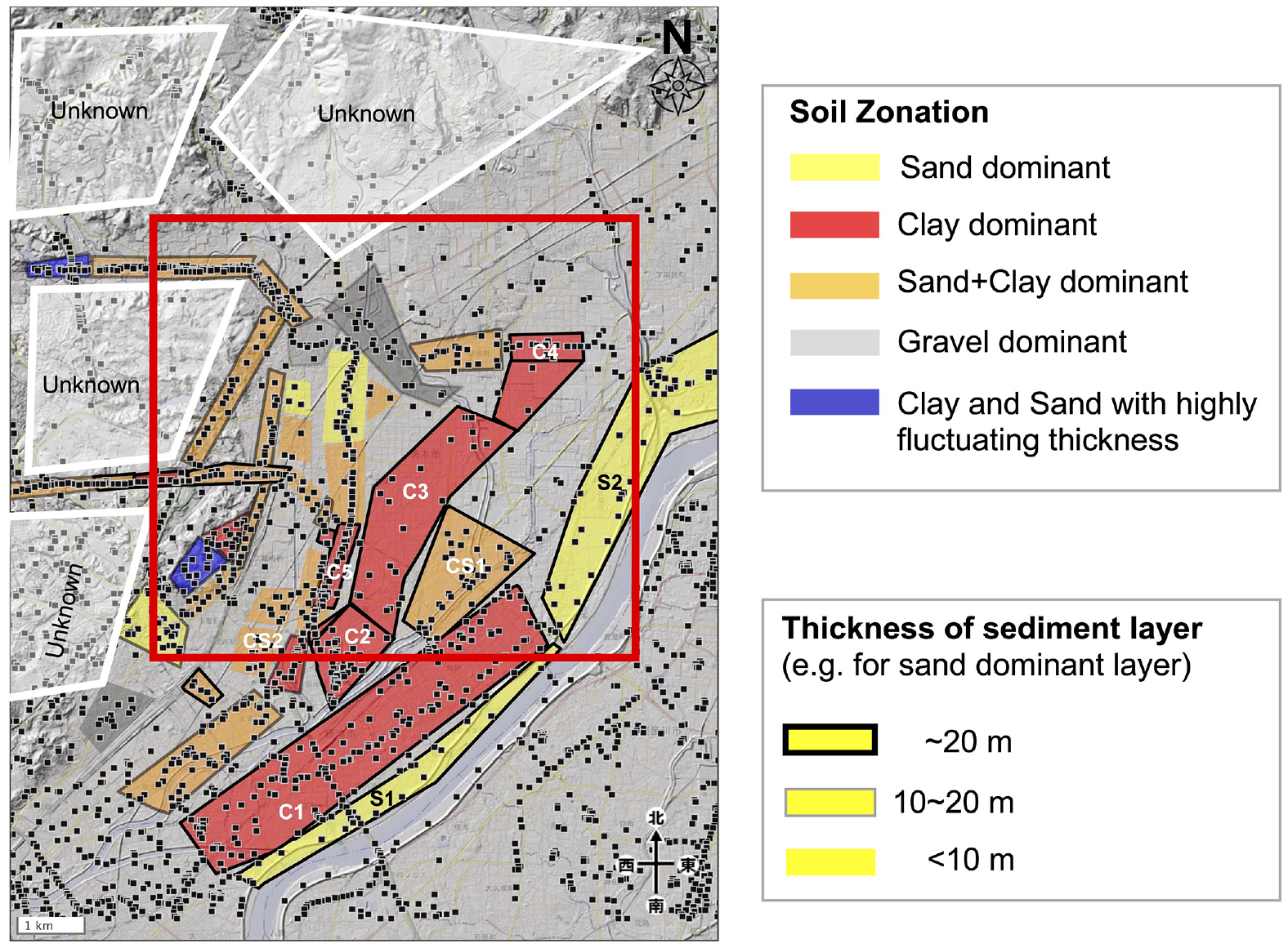
Soil zonation proposed in the study area. Please refer to the online version for color interpretation.
The zonation based on soil type highlights the presence or absence of a unique engineering bedrock. In zones where a unique engineering bedrock cannot be determined, the depth of the engineering bedrock or the sediment thickness will have high uncertainty. In Figure 9, all unmarked zones are zones with high uncertainty. However, in zones where a unique engineering bedrock can be defined, the depth of sediments does not vary significantly and can be modeled uniformly. In Figure 7, the following zones where a unique engineering bedrock can be defined are marked: S1, S2 (sand-dominant), C1, C2, C3, C4, C5 (clay-dominant), CS1, and CS2 (clay and sand dominant). In these zones, the uncertainty in the depth of engineering bedrock or the sediment thickness is low. Hence, the soil layers can be modeled with a representative soil column above the engineering bedrock.
Figure 10 explains the meaning of a representative soil column using five well-spaced sites from zone C1. At sites R1, R2, and R3, a thick and continuous gravel/sand layer exists below 20-m depth. At site R3, another thick sand layer exists below 35 m, but its continuity cannot be established due to insufficient data. So, based on the available data, the thick and continuous layer below 20-m depth can be safely assigned as the engineering bedrock. However, at sites R4 and R5, the information on the soil layers below 20-m depth is unavailable—the last available N-value for R5 hints at a stiff layer below 20 m. So, considering the similarity of the top layers (clay-dominant) of R4, R5 with top layers at R1, R2, and R3, and considering the possibility of a stiff layer below 20 m for R5, by applying engineering judgment, the layer below 20 m is assumed to be a “common layer” in this zone and extrapolated for R4 and R5. Thus, for zone C1, a representative soil column above the engineering bedrock can be proposed, as shown in Figure 10. The thickness of this soil column is about 20 m.
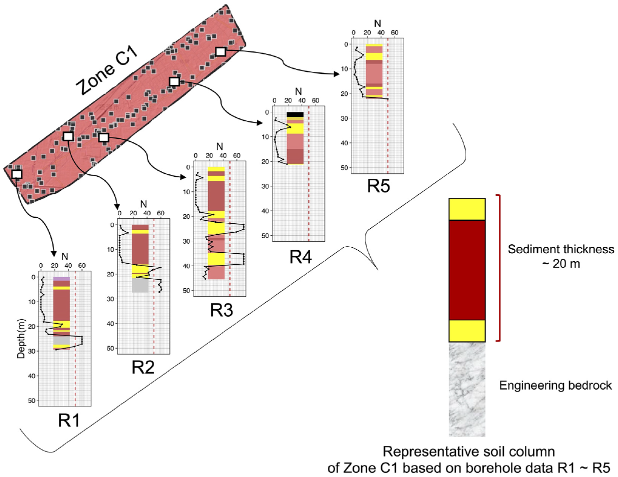
Representative soil column for clay-dominant zone C1. Please refer to the online version for color interpretation.
Thus, zoning helps assign a “common layer” as the engineering bedrock for selected zones and eases soil modeling with a representative borehole. In such zones, if engineering judgment allows sites with insufficient borehole depth could also be included, which are otherwise discarded for not being sufficiently informative.
In 1D seismic ground response analysis for evaluating the in-situ PGV site amplifications, the engineering bedrock is assumed as an elastic half-space, and the height of the soil columns above is used for the analysis. Figure 11a shows the histogram of the height of soil columns used for seismic ground response analysis in the study area. Figure 11b shows the spatial distribution of the depth of engineering bedrock in the study area. It is observed that the height of soil columns above the engineering bedrock (or the thickness of sediments) is not distributed uniformly in the study area. The right side of the study area is dominant with thicker sediments.
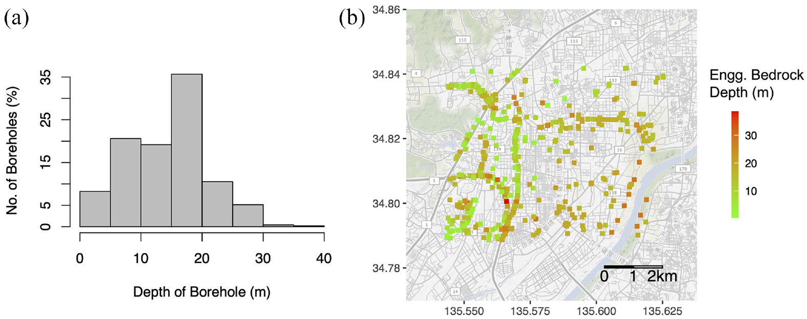
(a) Histogram of the height of soil columns used in seismic ground response analysis. (b) Distribution of engineering bedrock depth in the study area.
Results
In-situ PGV site amplification map
Figure 12 shows the means (
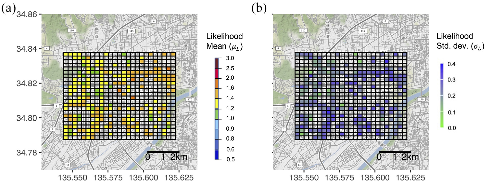
(a) Mean and (b) standard deviation for the likelihood site amplification. The mesh size is 250 m × 250 m.
The mesh-specific uncertainties in the in-situ PGV site amplifications (Figure 12b) arise from the variation of two factors: the borehole density and the input ground motion. When compared with Figure 11b, it is observed that the spatial distribution of mesh-specific uncertainties follows the thickness of sediments in sand and clay-dominant zones. The uncertainties at locations with thick sediment layers are higher than at locations with thin sediment layers. A possible reason is the higher variation of site amplification with input ground motions for a thicker soil column in 1D seismic ground response analysis. Also, another observation is that the local variation of this uncertainty is not uniform. On the right side of the study area, the local variation of uncertainty is very low. However, the uncertainty’s local variation is very high on the study area’s left side. When compared with the soil zonation map in Figure 9, it is seen that the right side of the study area coincides with the zones S1, S2, C1, C2, C3, C4, C5, CS1, and CS2, where the uncertainty in the depth of engineering bedrock is low. And the left side of the study area coincides with the unmarked zones where the uncertainty in the depth of engineering bedrock is high. Thus, the uncertainty information from the soil zonation is propagated to the in-situ PGV site amplification map.
Updating the proxy-based J-SHIS map
Using the Bayesian framework of UPM, the priors (Figure 5) are updated with the likelihoods (Figure 12). The posterior means (
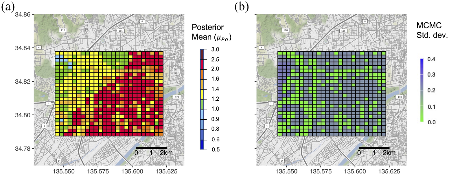
(a) Mean and (b) standard deviation of posterior estimations for representing finite sample uncertainty. The mesh size is 250 m × 250 m.
The map of the posterior means (
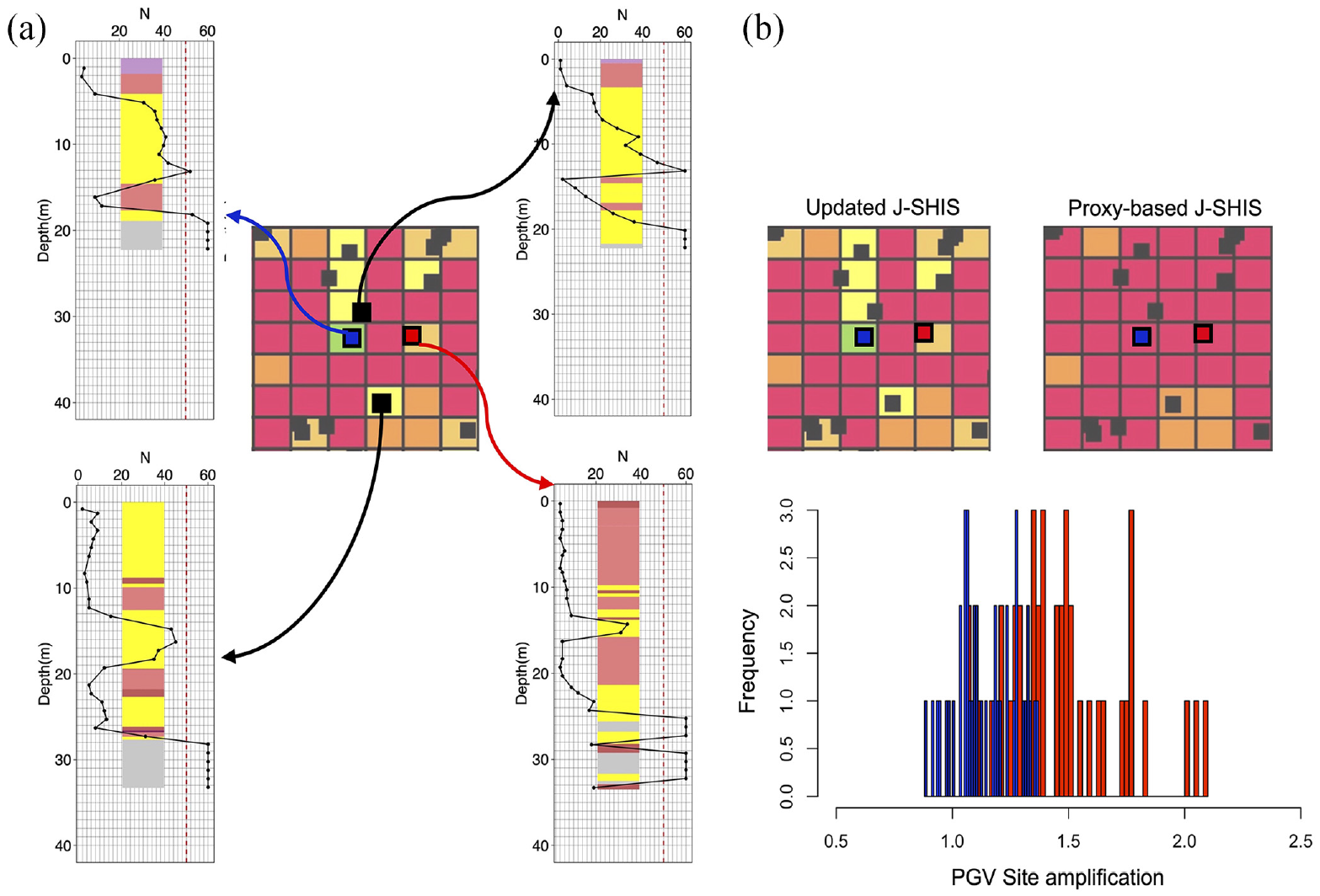
Figure 14 investigates three regions marked by D, D’, and E to understand the significance of the site amplification updates at the local scale. Figure 14a is the updated J-SHIS map, and Figure 14b is the proxy-based J-SHIS map. The mesh-size is 250 m × 250 m. In region D, the proxy-based J-SHIS map shows a sharp change from a high amplification area (in red) to a low amplification area (in blue). However, this contrast is significantly reduced in the updated map, and a smoother transition of mesh values is shown. In region D’, the sharp change from high amplification (in red) to low amplification (in blue) has not significantly changed in the updated map. The proxy-based J-SHIS map in region E shows uniform high amplification mesh values. However, the updated map shows a very low amplification area (in green).
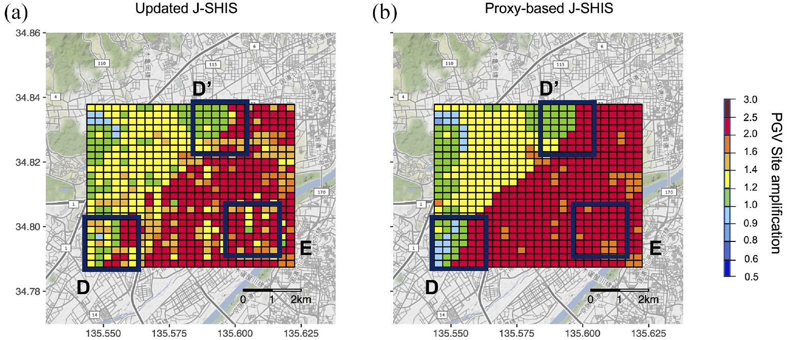
Comparison of updated and proxy-based J-SHIS map of site amplification. The mesh size is 250 m × 250 m. Regions D, D’, and E are further investigated in detail to understand the significance of the updates.
Figure 15 shows the locations of borehole data in regions D, D’, and E that can aid in understanding the aforementioned differences better. The mesh-size is 250 m × 250 m. Let us first focus on why the sharp change in region D has been updated, whereas the abrupt change in region D’ has not been updated. Region D has a high density of borehole data, which explains the increased granularity in the updated region D. However, in region D’, the borehole data density is not so high, which explains why region D’ is almost unchanged in the updated map. Thus, only available data areas are updated. The informative prior dominates the meshes where borehole data are not available.
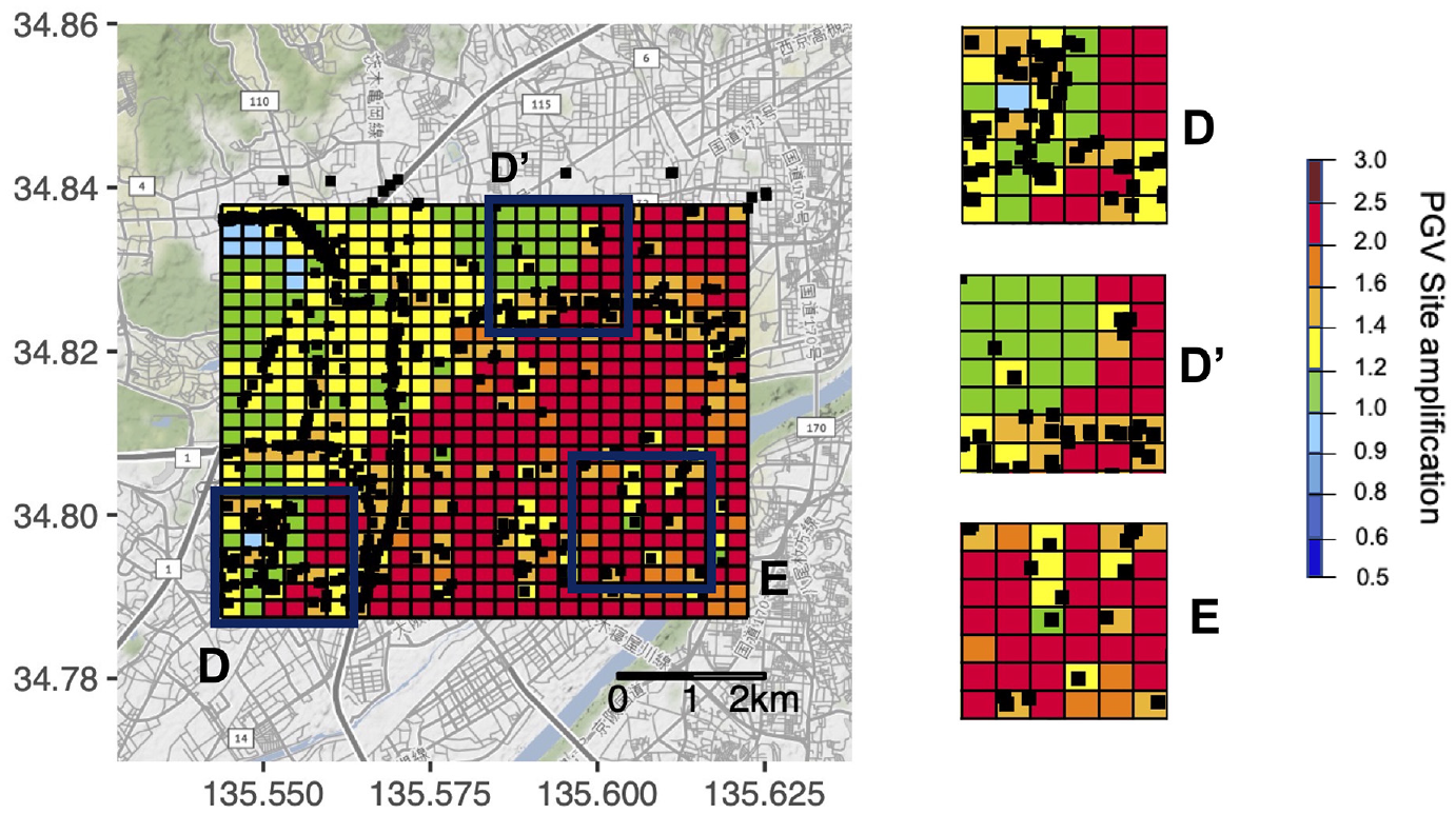
Borehole locations in regions D, D’, and E of the updated J-SHIS map. The mesh size is 250 m × 250 m.
Next, regions D and E updates are investigated in more detail. In region D, four borehole data are selected: two located in the high amplification area and two in the low amplification area of the proxy-based J-SHIS map, as shown in Figure 16a. No significant changes in sediment thickness can be observed, meaning there is uniformity in the site amplifications in this area. Figure 16b compares data distribution at two borehole locations, one from the high amplification (in red) and one from the low (in blue) amplification area. The overlapping data distributions also indicate no significant differences in the neighborhood mesh values, contradicting the sharp transition in the proxy-based J-SHIS map. As the updated map shows a smoother transition in this area, it can be concluded that it is appropriately updated based on borehole data.
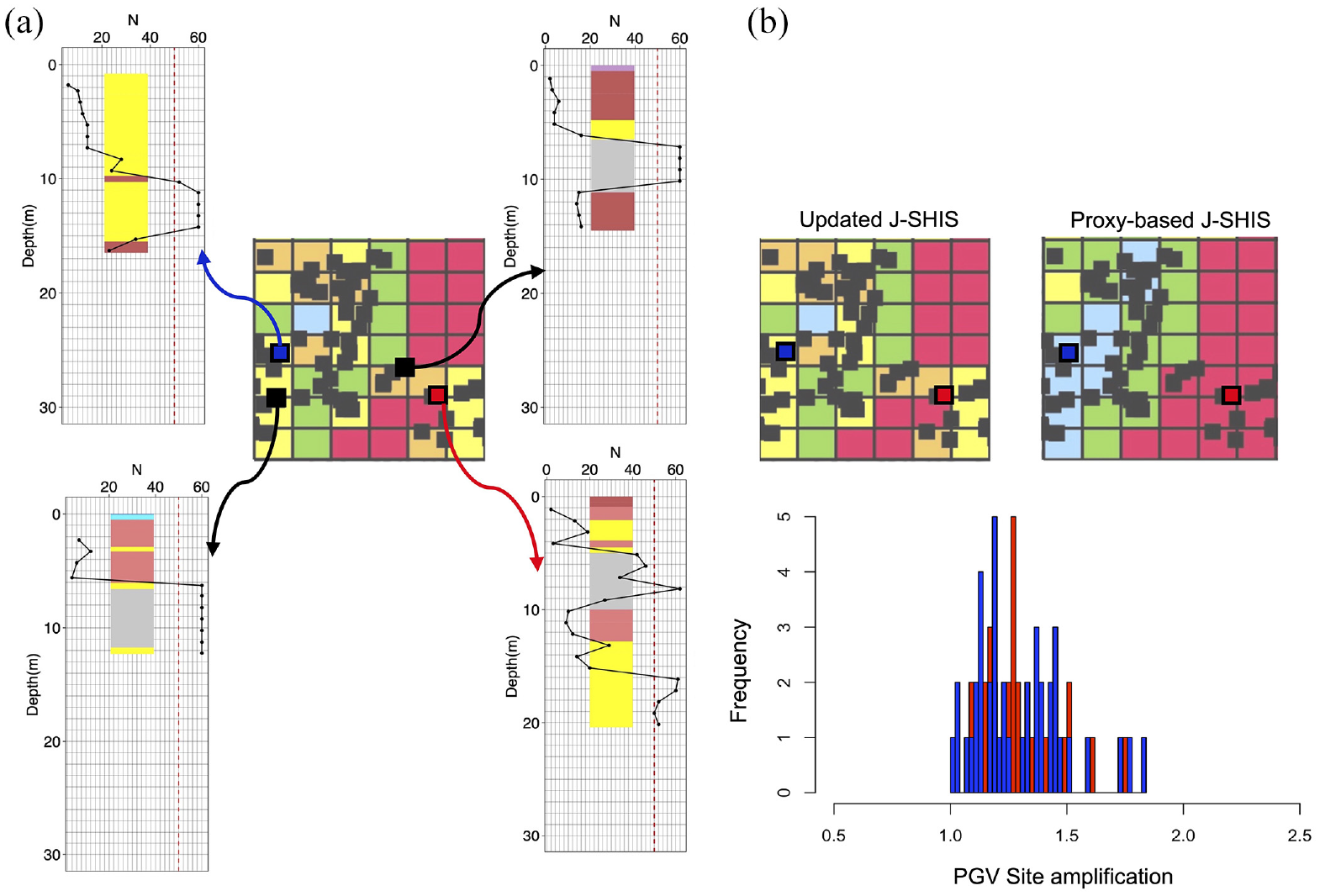
(a) Detailed borehole data in region D and (b) data distribution of site amplification for the two sites in red and blue. Please refer to the online version for color interpretation.
Region E is a transition region from a sand-dominated layer to a clay-dominated layer (Figure 9), where one would not expect uniform site amplifications. Another indication of non-uniform site amplification is the presence of two sites with substantially low sediment thickness and the other with higher sediment thickness (Figure 17). The updated map, thus, highlights significant local variations in the area, unlike the proxy-based J-SHIS map, which shows the whole area as uniform. Figure 17b compares the data distribution at two borehole locations that are almost non-overlapping (significantly high differences), indicating non-uniformity in the area and contradicting the uniform site amplifications in the proxy-based J-SHIS map. Since the updated map shows non-uniform site amplifications, it can be concluded that it is appropriately updated based on borehole data.
(a) Detailed borehole data in region E and (b) data distribution of site amplification for the two sites in red and blue. Please refer to the online version for color interpretation.
The updated map highlights the non-uniformity in site amplifications in areas with significantly high local variability. In addition, it smoothens the non-uniform site amplifications where the local borehole data are not significantly varying and follows the prior values where borehole data are missing. Thus, the updated map better represents the in-situ data and reflects appropriate updates to the proxy-based J-SHIS map. Although the strong informative priors limit the updates to only sites with in-situ data, this improvement is important in the local scale or scales important for micro-zonation studies. As more and more in-situ data become available, the scale of updates can be expanded to the regional or national scale to reflect more ground truth and less proxy-based estimates.
Discussions
Damage distribution during the 2018 Northern Osaka earthquake
It is essential to discuss how well the updated map aligns with the damage distribution observed during the 2018 Northern Osaka earthquake. Figure 18a shows the damage distribution based on Asano et al. (2021), where the damage is defined as follows:

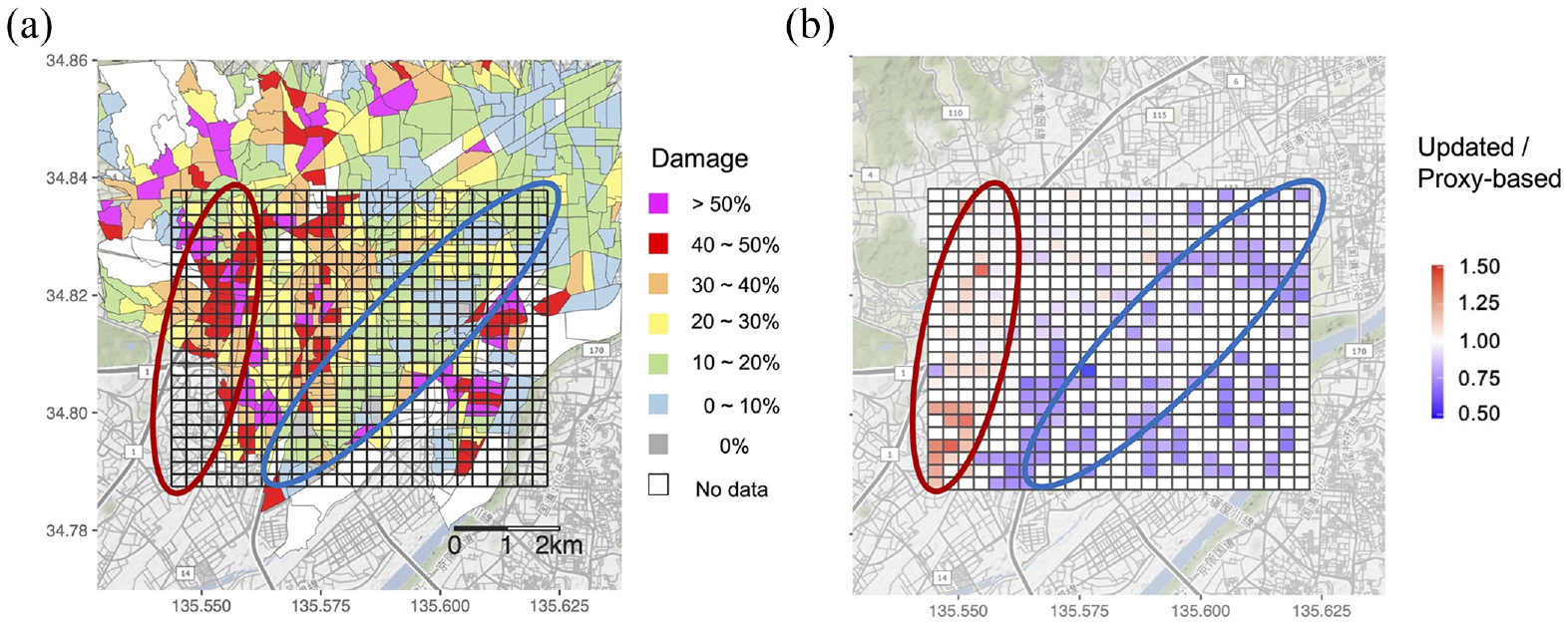
(a) Damage distribution during 2018 Mw 5.6 Northern Osaka earthquake from Asano et al. (2021) and (b) ratio map of updated to proxy-based J-SHIS site amplifications. The mesh size is 250 m × 250 m. Please refer to the online version for color interpretation.
A building damage certificate is proof of the extent to which the building was damaged. In Japan, house owners must procure several damage certificate proofs to be eligible for aid. The resolution of the damage map is Cho-Cho-Moku (in Japanese), the smallest unit of geographic area at the sub-municipality level in Japan.
Figure 18a shows that the damage areas are distributed across the study area. A zone with no damage also exists, as indicated by the blue circle. This zone lies in the previously high-amplification area of the proxy-based J-SHIS map. Also, as noted by the red circle, several damages exist in the previously low amplification area of the proxy-based J-SHIS map.
The proxy-based J-SHIS site amplification map uses PGV-based amplification as a metric of site amplification. As the objective of this study was to update the PGV-based J-SHIS site amplification map, the updated map is now also PGV-based. Also, the connection between site amplification and damage has been observed during previous earthquakes. In literature, several studies indicate that the earthquake damage pattern is more correlated to the PGV distribution than the PGA distribution. So, the PGV amplification metric was selected to investigate the role of site amplification in the damage observed during the 2018 Northern Osaka earthquake.
In Figure 18b, a ratio map is prepared to investigate how well the updated site amplifications can explain the observed damage. Each mesh represents the ratio of updated to proxy-based J-SHIS site amplifications in this map. The mesh-size is 250 m × 250 m. The blue circle corresponds to an area with lower amplification than the proxy-based J-SHIS map. These lower amplifications explain the presence of a no-damage area in the previously high amplification area of the proxy-based J-SHIS map. The red circle corresponds to an area with higher amplifications than the proxy-based J-SHIS map. These higher amplifications explain the presence of a high damage area in the previously low amplification area of the proxy-based J-SHIS map.
However, the updated map also shows lower amplifications in some areas of high damage. Thus, although the updated site amplifications could better explain damage in some previously low-amplification areas or the occurrence of no damage in one high-amplification area, they cannot explain the occurrence of all damage areas of the 2018 Northern Osaka earthquake.
Site amplifications alone might be unable to explain the damage distribution of the 2018 Northern Osaka earthquake. Further analysis is necessary to investigate the role of other factors in damage distribution. The damage distribution during an earthquake depends not only on the site amplification but also on factors such as the source directivity effect, age of buildings, etc. Kiyono et al. (2021) mention that the distribution of ground motions during the 2018 Northern Osaka earthquake cannot be explained by the site amplification alone. The role of rupture directivity needs to be investigated. Asano et al. (2021) attempted to discuss the damage distribution based on the age of buildings but could not explain the overall damage distribution. More research needs to be done to explain the damage distribution adequately.
One limitation of this study’s site amplification estimation method is the choice of input ground motions. Although the input ground motions are selected at sites that represent the engineering bedrock conditions, the input ground motions do not describe the same source-time characteristics of the 2018 Northern Osaka earthquake. Also, the input ground motions were applied uniformly at all borehole locations in the study area. However, during an earthquake, the input ground motions vary from one borehole location to another. Therefore, it is essential to investigate how these input ground motions influence the site amplification estimates and if the new estimates can explain the damage distribution. This map can be updated using the proposed scheme when more information is available.
The constraints from an informative prior
In the Bayesian updating scheme, the choice of a prior distribution dictates the posterior distribution. In general, non-informative priors are used to restrict the influence of the priors on the posteriors. Since our objective is to update the proxy-based J-SHIS map, it is considered the prior. The standard deviation of the prior distribution is determined based on the published values from Wakamatsu and Matsuoka (2013) and Fujimoto and Midorikawa (2006). The total standard deviation is very low, making the prior strongly informative, putting a strong constraint on the posterior distribution.
In UPM, the locations with no borehole data are usually mapped smoothly (uniform posterior estimates). This smooth map informs the user that there are no data points in that area and cautions about the confidence level in the map values. Since a strongly informative prior is used, which puts a heavy constraint on updates, the posterior map is not smoothened where the borehole data are unavailable but maintains the prior proxy-based values. Thus, the strong priors restrict us from showing the full effects of the density of boreholes in the site amplification estimates. More studies must be done on the appropriate choice of priors when updating the proxy-based maps with borehole data.
Scope of application
This study introduces a data-driven approach to updating proxy-based site amplification maps with available borehole data. This initial attempt at building a data-driven site amplification map has generated promising results.
Although there are limitations that need to be addressed in future research, the results from this study are significant from the perspective of regional seismic hazard and risk assessment.
In addition, real-time estimation tools, such as ShakeMap and PAGER, where the increased accuracy positively impacts the process of post-earthquake emergency management, can also benefit from accurate regional scale site amplification data (Earle et al., 2008; Wald et al., 1999, 2008).
Decisions to mitigate earthquake-related damages and losses are based primarily on the site amplification maps. Thus these maps are a vital component of the decision-making process. The data-driven approach introduced in this study generates a site amplification map that reflects the significance of local in-situ data variability. In-situ amplifications are non-uniform (high spatial resolution) when the local differences are significant. Conversely, in-situ amplifications are uniform when the local differences are insignificant, or the data availability is low (low spatial resolution). In a way, the local spatial resolutions generated by this data-driven approach reflect the confidence level of the site amplification estimates. Confidence can add value to the data used for decision-making. Hence, the site amplification map generated with this data-driven approach will add value to the site amplification data used for decision-making in areas with high spatial resolution. Conversely, it will highlight the need for more data before using it for decision-making in areas with low spatial resolution.
Summary
Proxy parameters like engineering geology, Vs30, and so on, are frequently used for preparing site amplification maps. However, these proxy-based maps do not always reflect the in-situ conditions. For example, during the 2018 Mw 5.6 Northern Osaka earthquake in Japan, damage distribution in Osaka’s Ibaraki and Takatsuki cities significantly deviated from the site amplification estimations of the proxy-based J-SHIS map. One possible explanation for the deviation is the difference between proxy-based estimations and in-situ site amplification values. The other factors that could play a role in the observed divergence are strong ground motions, source effect, age of buildings, and so on. In this study, the role of site amplification in the damage distribution is investigated with the site amplification evaluations from borehole data.
A Bayesian updating scheme is proposed for updating the proxy-based J-SHIS map with borehole data. The proposed scheme is based on UPM, where posterior estimates correspond to the significance of local variabilities and the denseness or sparseness of the available borehole data. The study area is in the Ibaraki and Takatsuki cities of Osaka, located close to the earthquake’s epicenter, where dense borehole data from the Kansai Geo-informatics Network are available. In-situ site amplifications at the borehole locations are evaluated using equivalent linear ground response analysis with non-linear soil modeling. Finally, the updated map or the posterior in Bayesian inference is generated with proxy-based J-SHIS values as priors and evaluated in-situ site amplifications as likelihoods.
The updated map shows increased spatial granularity in previously low- and high-amplification regions. Site amplifications are updated only at meshes with borehole data. In meshes with no borehole data, the informative prior dominates. The updated map highlights non-uniform site amplifications at areas where the in-situ data shows significantly high local variabilities. Uniform site amplifications are generated in areas where the in-situ data show no significant local variabilities. The updated map is a better representation of the in-situ data. In the updated map, the uncertainties arising from the significance of local in-situ data variability and the mesh-specific density of borehole data drive the posterior estimates.
Although the updated site amplifications could better explain the damage in some previously low amplification areas or the occurrence of no damage in once high-amplification area, they cannot explain all the damage areas of the 2018 Northern Osaka earthquake. Site amplifications alone might be unable to explain the damage distribution of the 2018 Northern Osaka earthquake. Further analysis is necessary to investigate the role of other factors, such as the source directivity effect, age of buildings, and so on, in the damage distribution.
Footnotes
Acknowledgements
The authors thank the Geo-research Institute in Osaka, Japan, for providing us with the borehole data. The authors are grateful for three anonymous reviewers’ suggestions and comments, who helped improve the manuscript’s quality.
Declaration of conflicting interests
The author(s) declared no potential conflicts of interest with respect to the research, authorship, and/or publication of this article.
Funding
The author(s) disclosed receipt of the following financial support for the research, authorship, and/or publication of this article: This work was supported by KAKENHI, Japan Society for the Promotion of Science (grant nos. 19H02224 and 23H01492).