Sediment thickness map of United States Atlantic and Gulf Coastal Plain Strata,and their influence on earthquake ground motions

Abstract

With the recent successful accounting of basin depth ground-motion adjustments in seismic hazard analyses for select areas of the western United States, we move toward implementing similar adjustments in the Atlantic and Gulf Coastal Plains by constructing a sediment thickness model and evaluating multiple relevant site amplification models for central and eastern United States seismic hazard analyses. We digitize and combine existing sediment thickness data sets into a composite surface that delineates the base of Cretaceous sediments under the Atlantic Coastal Plain and the base of Mesozoic sediments under the Gulf Coastal Plain. Amplification models dependent on sediment thickness, site natural period, and source-to-site path length are compared with data sets of observed ground motions to evaluate the ability of the new models to improve ground motion estimates. We find that the amplification models can account for observed trends in sediment-thickness and period-dependent residuals, but some tuning is required. For example, the model of Chapman and Guo requires a reference V_S30, the time-averaged shear-wave velocity within 30 m of the Earth’s surface, for non-Coastal Plain sites, which we estimate to be between about 1 and 2 km/s. Along with our sediment thickness model, we estimate a velocity profile for application to the Harmon et al. site-natural-period-based model in order to best match the Chapman and Guo period dependence for a broad range of sediment thicknesses. The Next Generation of Attenuation models for the eastern United States Gulf Coast path-based adjustment models can also account for seismic attenuation in the Coastal Plain sediments and reduce the standard deviation of total residuals. If enacted in the U.S. Geological Survey National Seismic Hazard Model, these amplification models will reduce predicted short-period (<1 s) and increase predicted long-period (>1 s) ground motions in the Coastal Plains appreciably.

Introduction

Ground-motion models (GMMs) developed for the western United States (WUS) account for basin depth via the depths to 1.0 and 2.5 km/s shear-wave velocity (Bozorgnia et al., 2014). In the 2018 U.S. Geological Survey (USGS) National Seismic Hazard Model (NSHM), Petersen et al. (2020) leveraged this improvement for select areas in the WUS where basin depth information is available (Powers et al., 2021): Los Angeles and the San Francisco Bay Area basins in California, the Puget Sound region in Washington, and the Wasatch Front area in Utah. Steps are now being taken by members of the USGS NSHM project to improve estimates of earthquake ground shaking in the central and eastern United States (CEUS) by accounting for the thick sediment deposits beneath the Atlantic and Gulf Coastal Plains.

The effects of thick Coastal Plain sediments on earthquake ground motions have been recognized for some time (e.g. Bodin and Horton, 1999; Chapman et al., 2003 and references therein; Hashash and Park, 2001). The 2011 M5.7 Mineral, Virginia earthquake, for example, highlighted unique ground-motion effects along the northern Atlantic Coastal Plain (Hough, 2012) and in Washington, D.C. (Pratt et al., 2017), where large structures, including the Washington Monument and National Cathedral that sit over thick packages of relatively soft sediment, were damaged (Wells et al., 2015). More broadly, the passage of USArray through the Coastal Plains beginning in 2011 yielded extensive observations of high-frequency seismic attenuation (Chapman and Conn, 2016; Cramer, 2018) and low-frequency amplification (Guo and Chapman, 2019).

During development of the Next Generation of Attenuation models for the eastern United States (NGA-East; Goulet et al., 2021a), the most recent effort to formulate GMMs for central and eastern North America, a working group considered how the Gulf Coastal Plain sediments affect earthquake ground motions and found that the thick sediments attenuated shaking (Goulet et al., 2018; Hollenback et al., 2015). They suggest that the amount of attenuation increases with the length of the source-to-site path through the Coastal Plain sediments, for which they provided two polygons covering differing extents of the Gulf Coastal Plain. They propose two models, one that is independent of shaking period and another in which attenuation increases with oscillator frequency. More recently, Guo and Chapman (2019) and Pratt and Schleicher (2021) found that estimates of earthquake ground motions on the Coastal Plain sediments could be improved by accounting for the depth to the geologic basement where shear-wave velocities jump to around 3.5 km/s (Chapman et al., 2006; Schmandt and Lin, 2014; Shen and Ritzwoller, 2016).

Guo and Chapman (2019) show that the effect of the Coastal Plain sediments on the Fourier amplitude spectrum of the Lg phase is a complex interaction of amplification due to systematically increasing velocity with depth in the sediments and to strong anelastic attenuation of the sediments. Both effects are frequency-dependent, with lower frequencies being amplified and higher frequencies being attenuated in the Coastal Plain, relative to average site response outside the Coastal Plain. The high-frequency attenuation is treated by Guo and Chapman (2019) using a kappa model, that is, an increasing function of sediment thickness. They find average differential kappa values between Coastal Plain and non-Coastal Plain sites that exceed 0.1 s at 10-km sediment thickness, consistent with the previous study by Chapman and Conn (2016). Low-frequency amplification in the Guo and Chapman (2019) model also depends on sediment thickness, with the frequency of the maximum site amplification being inversely related to the thickness of the sediment section.

To implement Coastal Plain sediment-thickness-based amplification models in the NSHM, it is ideal to develop a seamless surface that covers the entirety of the Coastal Plains and is consistent with the depths used in the amplification models. Mooney and Kaban (2010) published a sediment thickness map for all of North America, which is attributed to the map by Weiner et al. (1985) and work of Frezon et al. (1983). Guo and Chapman (2019) and Pratt and Schleicher (2021), however, used more region-specific sources (Herrick and Vorhis, 1963; Lawrence and Hoffman, 1993; Powars et al., 2014; Salvador, 1991; Wait and Davis, 1986). We compile many of these (Mills et al., 2020) and additional sources (Campbell and Coes, 2010; North Carolina Division of Water Resources (NCDWR), 2020; Pope et al., 2016) to produce a uniform-resolution sediment thickness model for evaluating ground-motion effects across the region and for the potential implementation of site amplification models into the USGS NSHM.

We consider three sets of pseudo-response spectral acceleration (PSA)-based amplification models to evaluate the effect of these sediments on ground motion characterization in the NSHM. These include (1) the Chapman and Guo (2021) model, hereafter termed “CG21,” which extended the Fourier-based model of Guo and Chapman (2019) that relates Fourier spectral amplitudes to sediment thickness; (2) the Harmon et al. (2019a) models, which use a modular approach dependent on sediment thickness and site period drawing from an amplification data set of large-scale one-dimensional (1D) site response analyses (Harmon et al., 2019b); and (3) the NGA-East model (Goulet et al., 2021a), in which attenuation is dependent on the length of the path within the Gulf Coastal Plain sediments. We compile an updated data set of ground-motion records (since just before the end of NGA-East in 2011) that we use together with two previous compilations and the sediment thickness model developed in this article to evaluate the three sets of models.

Sediment thickness

A map of the extent and thickness of Coastal Plain sediments above basement rocks is needed to apply sediment-thickness-based amplification models in the USGS NSHM. On the Atlantic Coastal Plain, this map is defined as the thickness of Cretaceous and younger post-rift sediments. On the Gulf Coastal Plain, this map is defined as the thickness of Mesozoic and younger syn- and post-rift sediments. Relatively narrow and isolated Mesozoic rift basins beneath the Atlantic Coastal Plain (e.g. Withjack et al., 1998) are not included because their subsurface geometry is not well characterized, and their effects on ground motions are not well studied. Furthermore, the model of Harmon et al. (2019a) based on site natural period requires a conversion from sediment thickness to site period via a velocity profile, the derivation of which is discussed in the section titled “Harmon and others.”

Developing a composite surface model

Maps of the elevation of the basement beneath syn- and post-rift sediments were collected for the Gulf and Atlantic Coastal Plains, respectively. A total of six paper maps containing basement elevation contours and contact elevations within wells and along seismic lines were scanned and rectified and digitized in ArcGIS (Mills et al., 2020). To supplement these maps, we downloaded two Atlantic Coastal Plain hydrogeologic reports in which the base of Cretaceous rocks was identified (Campbell and Coes, 2010; Pope et al., 2016), in addition to elevations of the base of Cretaceous rocks in 162 wells from the NCDWR (2020; Figure 1). For all other areas, we use the basement map of Mooney and Kaban (2010), which was constructed from the maps produced by Weiner et al. (1985) and the work of Frezon et al. (1983).

Figure 1.

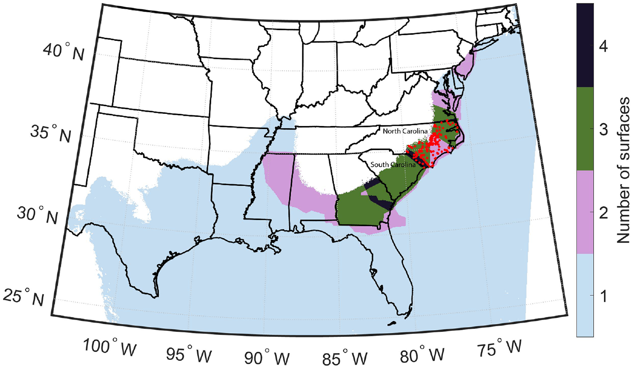
The number of sediment thickness surfaces that are combined at each location within the Coastal Plains. Also shown are the locations of wells in North Carolina with basement depths (dots).

The following workflow (Figure 2) details the development of the composite surface. In step 1, we define an elevation contour (General Bathymetric Chart of the Oceans (GEBCO), 2018) that reflects the landward extent of Coastal Plain sediments based on the contact between Cretaceous rocks and older sedimentary or igneous units as depicted in the USGS compilation of State geologic maps (Horton et al., 2017). In central and southern Texas, this contour is adjusted to roughly match the extent of Coastal Plain sediments as depicted by Guo and Chapman (2019). We refer to this contour as the zero-thickness contour. In step 2, we draw a polygon around each individual elevation data set and the updip zero-thickness contour. For step 3, we produce a 1-km gridded surface representing the elevation at the top of basement rocks for each data set. Within the polygon defined in step 2, we use cubic interpolation. Outside the polygon across the full extent of the Coastal Plain, we use nearest-neighbor extrapolation to assign elevation values and facilitate a smooth transition to neighboring data sets. In step 4, we combine the elevation surfaces from all of the data sets in a weighted average, where each surface is given a weight of one within its respective polygon (step 2), and outside its polygon, where the surface is extrapolated, the weight is tapered to zero over a short distance. There is some overlap between data sets, and the maximum number of available surfaces with full weight at any given location is four (Figure 1). The composite elevation surface is then subtracted from the Earth’s surface elevation to produce a sediment thickness map (Figure 3).

Figure 2.

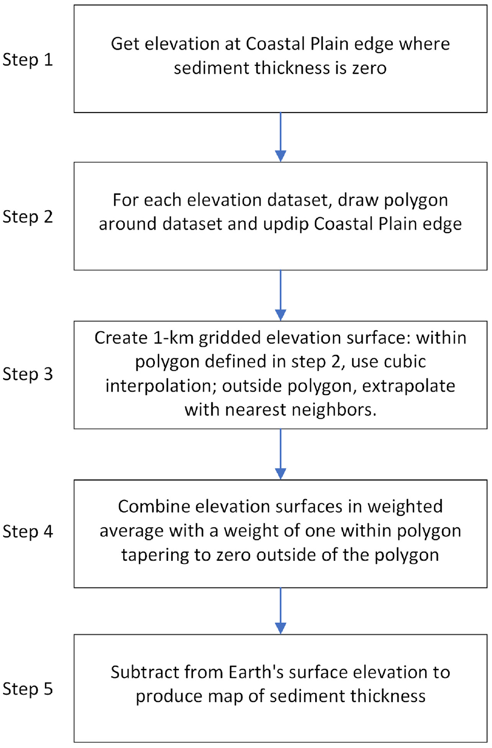
Flow chart outlining the five steps to generate the Coastal Plain sediment thickness map.

Figure 3.

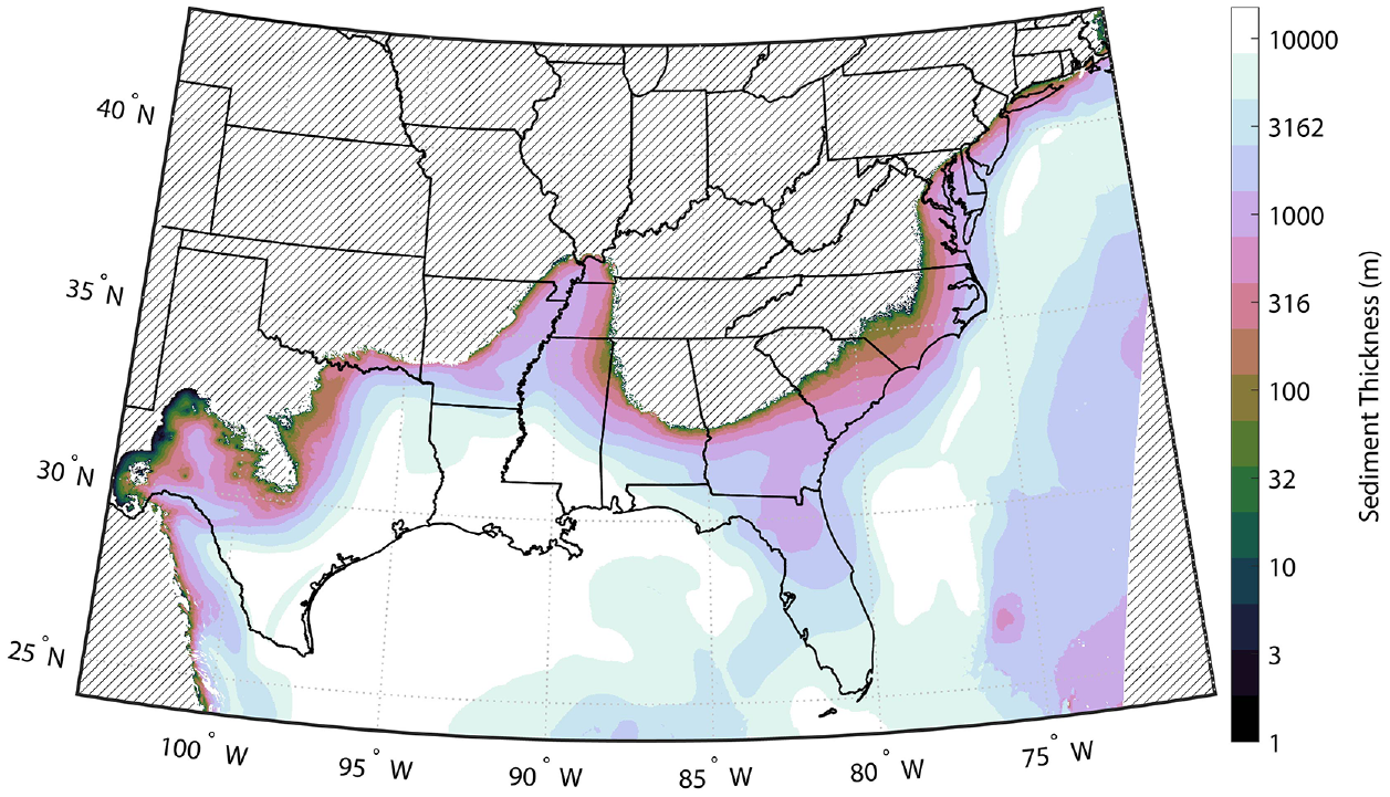
Composite sediment thickness map in meters across the Atlantic and Gulf Coastal Plains. The hatched area is outside of the Coastal Plains or undefined.

Uncertainty

There is geographic overlap between several studies, each of which may have had access to different data sets (seismic reflection and/or well data) and interpreted and contoured the data differently, resulting in variations in the elevation of the basement surface. We use this variability as an estimate of the epistemic uncertainty in the thickness of syn- and post-rift sediments (Figure 4). Half of the locations have a natural log standard deviation less than 0.07 (factor of 1.07 uncertainty, i.e. e^0.07), and 95% have less than 0.37 (factor of 1.45 uncertainty). However, we find that the variability increases with decreasing sediment thickness, h. For locations with h greater than 500 m, half of the locations have a natural log standard deviation, σ_lnh, less than 0.06 (factor of 1.06 uncertainty, i.e. e^0.06), and 95% have less than 0.3 (factor of 1.35 uncertainty). For h less than 500 m, standard deviations increase steadily as sediments approach zero thickness, with half of the locations having σ_lnh less than 0.1 (factor of 1.11 uncertainty) and 95% less than 0.6 (factor of 1.82 uncertainty). Regarding the spatial distribution of uncertainty, several small discrete locations differ between input surfaces in the Atlantic Coastal Plain, whereas more widespread differences between thickness models are present in the Gulf Coastal Plain, particularly in southern Alabama. These discrepancies cannot be resolved until additional data are obtained, but their locations can be used to prioritize future data collection efforts.

Figure 4.

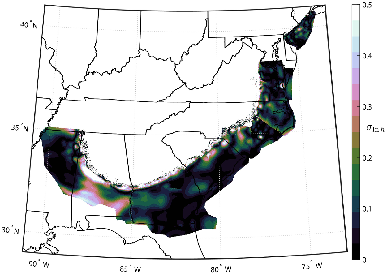
Variation between estimates of basement elevation, σ_lnh, determined from locations where two or more studies are present. Unshaded locations represent areas with only one study or those that are outside the Coastal Plain region (Figure 1).

Comparison with Guo and Chapman

The composite map was not available at the time of the Guo and Chapman (2019) or the initial Pratt and Schleicher (2021) studies. Pratt and Schleicher (2021) subsequently used a prior version of this surface, but it has since been updated to include the work of Mooney and Kaban (2010). This update had little effect on the work of Pratt and Schleicher (2021) because they concentrate on seismic stations on the Atlantic Coastal Plain, and the use of Mooney and Kaban primarily affects the deeper parts of the Gulf Coast province and offshore areas. Regardless, it is important that sediment thickness values used to implement attenuation/amplification models are consistent with the sediment thickness values used in these amplification studies.

We find that the sediment thicknesses used in the Guo and Chapman (2019) study, which provided the basis for the amplification model in Chapman and Guo (2021), are consistent with our sediment thickness map (Figure 5). This is not entirely unexpected given that most of the paper maps that were consulted for their amplification study were digitized in the work by Mills et al. (2020) and used here to produce the composite surface. This indicates that the composite surface can be used with these amplification studies in seismic hazard analyses without introducing significant bias.

Figure 5.

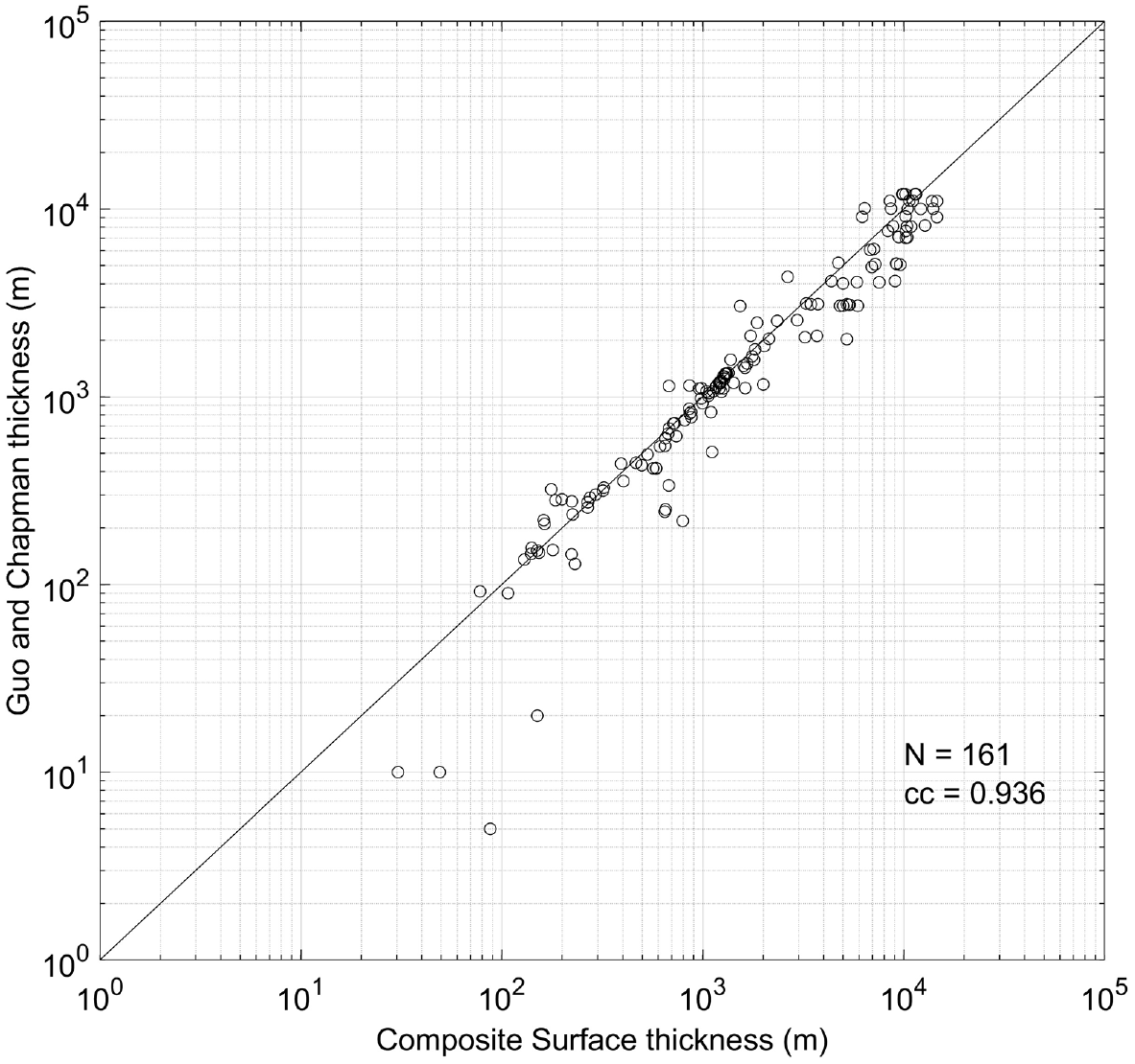
Comparison of 161 sediment thickness values used in Guo and Chapman (2019) plotted against those extracted from the composite map. The correlation coefficient (cc) between the two data sets is 0.936.

Ground-motion data set comparison

Overview

We evaluate available amplification models applicable to the Coastal Plain areas using two data sets that were previously compiled, in addition to a new data compilation for the CEUS (Figure 6). The NGA-East data set (Goulet et al., 2021b) was developed as part of an effort to update CEUS GMMs, which were then used in the 2018 USGS NSHM (Petersen et al., 2020). The data set consists of ground motions from 82 earthquakes with magnitude (M) 2.2 to 6.8 occurring prior to 2012 measured at 1268 stations out to 3500 km distance, yielding 9382 records. We also have the Chapman and Guo (2021) data set, which contains ground motions from 17 earthquakes with M3.9 to 5.7 from 2010 to 2018, measured on 629 stations out to 1000 km and yielding 2367 records.

Figure 6.

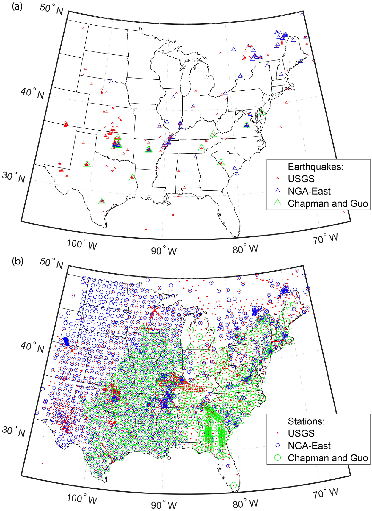
(a) Earthquakes (triangles) and (b) station locations (dots and circles) for the three data sets considered in this study: USGS (Thompson et al., 2023)—small symbols; NGA-East (Goulet et al., 2021b)—medium symbols; and Chapman and Guo (2021)—large symbols.

We supplement available ground-motion data sets from the CEUS with updated records from recent earthquakes (USGS data set in Figure 6). The updated ground-motion data set (Thompson et al., 2023) includes earthquakes with M3.1 to 5.8 occurring from 2010 to 2020 in the CEUS with data available through the Incorporated Research Institutions for Seismology (IRIS) and the Center for Engineering Strong Motion Data (CESMD). Because the NGA-East data set ends in 2011, the updated data set comprises records for the past ∼10 years from the region and includes many stations from the USArray Transportable Array in the CEUS that were not installed at the time of the NGA-East data processing.

Ground-motion records were compiled and processed with the gmprocess Python package developed by Hearne et al. (2019) and previously applied in multiple regions (e.g. Moschetti et al., 2021; Rekoske et al., 2020). The automated processing methods use standard strong-motion processing workflows (e.g. Goulet et al., 2021b; Rekoske et al., 2020): raw time series data are screened for waveform clipping (Kleckner et al., 2022), instrument-response corrected, band-pass filtered using corners determined by signal-to-noise ratios, windowed, and baseline corrected. We measure peak ground acceleration and velocity and horizontal PSA at 21 oscillator periods between 0.01 and 10 s in terms of the median intensity of horizontal ground-motion components rotated through 180° (RotD50; Boore, 2010). Site metadata for V_S30 (the time-averaged shear-wave velocity within 30 m of the Earth’s surface) (Heath et al., 2020) and sediment thickness—from the compilation described above—are associated with all records. Various magnitude scales are converted to moment magnitude using the rules established by the Central and Eastern United States Seismic Source characterization for nuclear facilities (CEUS-SSCn, 2012). We further screen PSA for outliers, which may be present due to incorrect instrument response metadata or transient sources of noise present within the signal window. Incorrect instrument response metadata may be present during a station’s entire deployment or only over certain periods of time, if, for example, instrumentation is changed but metadata are not updated. We identified and removed about 1000 of these records from 77 stations. When noise sources are present, they tend to affect the highest and lowest frequencies. In these cases, we effectively narrow the band over which to consider ground motions from these records, of which there are 37 records from 30 stations. Finally, we discard short-period stations with the channel name EH, which tend to have unusual spectra and require further investigation. There are 2785 of these records from 318 stations.

The final data set consists of 269 earthquakes measured on 2799 stations out to 1000 km, yielding 38,400 records. We limit stations to 1000 km epicentral distance to reduce the potential for sampling bias from unusually strong ground motions at large distance (Contreras et al., 2022). Of the 2799 stations in this data set, 550 are on the Coastal Plains. There is some limited overlap of events and stations between the three data sets, and they each have recording stations on the Atlantic and Gulf Coastal Plains. For the same event and station combination, the three data sets give similar spectral accelerations with nearly identical average accelerations around 1-s period. At 0.1- and 10-s period, however, the USGS data set has greater average ground motions (Supplemental Figure S1) than Chapman and Guo (2021) and NGA-East (Goulet et al., 2021b). Short- and long-period discrepancies could be due to differences in the many processing decisions that are made and is the subject of ongoing study (Schleicher et al., 2023). In particular, the short-period discrepancies could be due to differences in how time series are upsampled prior to computing response spectra (Boore and Goulet, 2014).

Between rupture distances of 100 and 1000 km, the three data sets have a relatively uniform distribution of Coastal Plain records (Supplemental Figure S2). Most of the records are from earthquakes having magnitudes between 3 and 5 with each data set having a few larger events (Figure 7). In addition, the NGA-East data set has six close-in records from two earthquakes below M3. Regarding Coastal Plain sediment thickness, a large range is well sampled in each data set.

Figure 7.

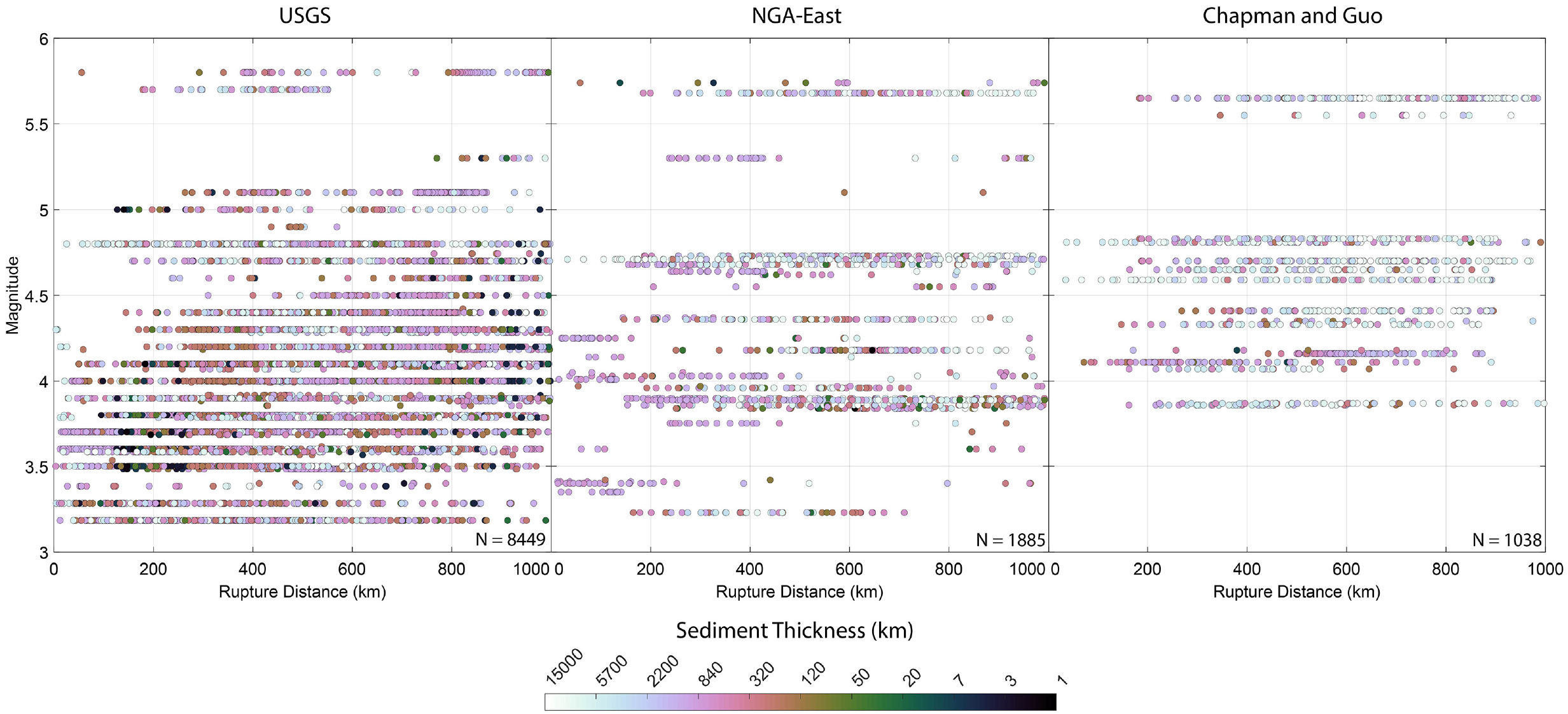
Magnitude versus rupture distance colored by sediment thickness for each Coastal Plain record in the three data sets. Also noted in the lower right-hand corner of each figure are the number of Coastal Plain records for each data set.

Residual dependence on period and sediment thickness

We compare these data sets to predictions by computing model residuals, which are defined as the difference between the natural log of the observed ground motion and the natural log of the GMM prediction. Predicted ground motions account for magnitude and distance using the NGA-East weighted average of the final recommended 17 Sammon’s mapping-based GMMs for 5% damped PSA on a hard-rock reference site having a V_S30 of 3000 m/s (Goulet et al., 2021a). This average model is based on a set of 18 seed models produced by independent GMM developers, which were derived primarily from simulations that incorporated existing research on earthquake stress drop, geometric spreading, and crustal attenuation for regions outside of the Coastal Plains. Ground-motion model predictions for each period in the median model are extrapolated to magnitudes less than 4 using MATLAB’s modified Akima cubic formulation in two dimensions (magnitude and natural log of the distance; Supplemental Figure S3); no apparent magnitude-dependent trends in the residuals are introduced (Supplemental Figure S4), and the extrapolation produces results similar to what is done for the USGS ShakeMap product (Worden et al., 2020).

From the set of stations in Figure 6b located on the Coastal Plains (i.e. where Coastal Plain sediment thickness is greater than zero), all three data sets exhibit total ground-motion residuals having a strong dependence on period (Figure 8): long periods are amplified, and short periods are attenuated relative to the model. Larger residuals for the USGS data set relative to the other two at periods between about 0.1 and 1 s are due to the USGS data set having a relatively greater number of stations on sites with less thick sediment. With regard to sediment thickness (Figure 9), there is a negative trend in residuals with increasing sediment thickness at shorter periods (<∼2 s) and a positive trend at longer periods.

Figure 8.

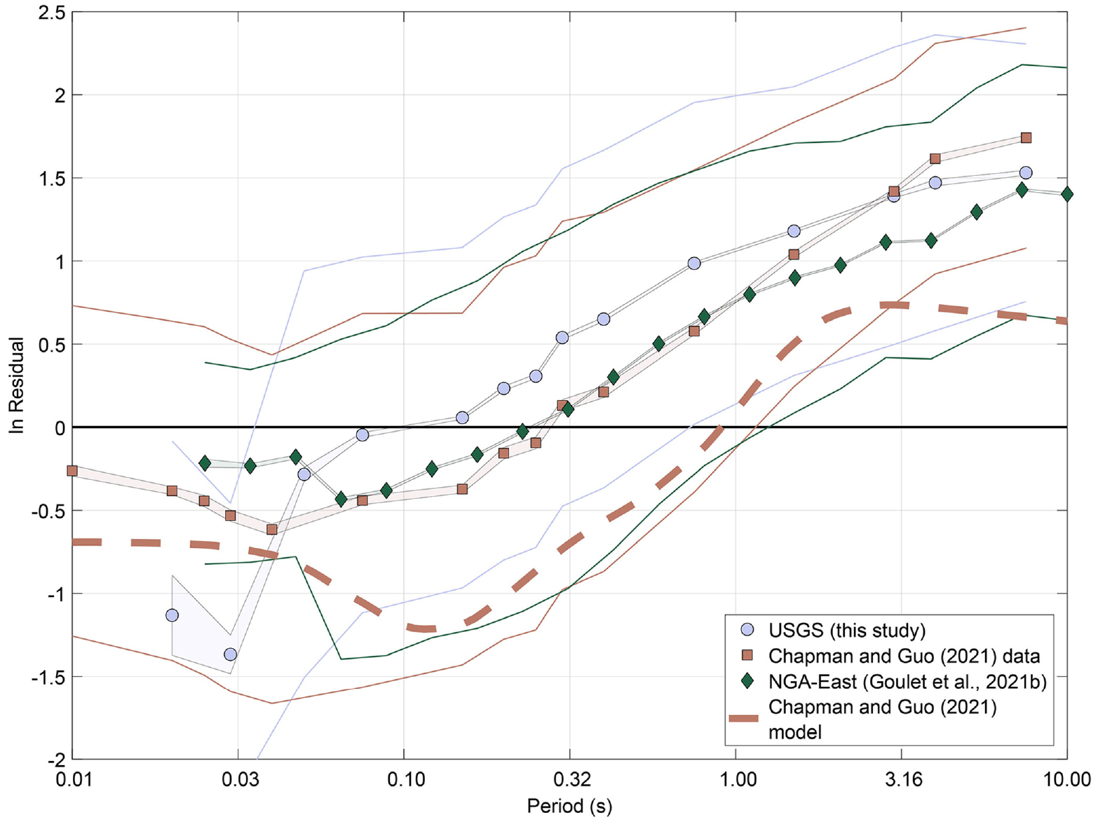
Total ground-motion binned-average PSA residuals relative to the NGA-East median model for the reference rock condition for the three data sets at Coastal Plain sites as a function of oscillator period. Solid lines encompass ± 1 standard deviation of residuals within each bin, and shaded areas encompass ± 1 standard error. Also shown is the CG21 model (thick dashed line). To facilitate this comparison with CG21, we use in this model the mean magnitude (4.6), distance (550 km), and sediment thickness (4.9 km) at Coastal Plain stations from the Chapman and Guo (2021) data set. Note that CG21 is relative to an average non-Coastal Plain site condition, which accounts for the offset between observed and modeled ground motions.

Figure 9.

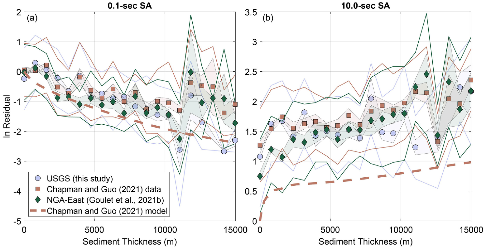
Total ground-motion binned-average pseudo-response spectral acceleration (SA) residuals relative to the NGA-East median model for the reference rock condition for the three data sets as a function of Coastal Plain sediment thickness at (a) 0.1-s and (b) 10-s oscillator periods. Thin lines encompass ± 1 standard deviation of residuals within each bin, and shaded areas encompass ± 1 standard error. Also shown is the CG21 model (thick dashed line) for the mean magnitude (4.6) and distance (550 km) at Coastal Plain stations in the Chapman and Guo (2021) ground-motion data set. Note that CG21 is relative to an average non-Coastal Plain site condition, which accounts for the offset between observed and modeled ground motions.

Comparison of data with attenuation/amplification models

CG21

To facilitate a basic comparison, we assume in the CG21 model an average magnitude (4.6), distance (550 km), and sediment thickness (4.9 km; Figure 8 only)—averages determined from the CG21 ground-motion data set. We find that the CG21 model with these parameter values matches the observed trends well (Figures 8 and 9), but generally lies below the observed residuals. Part of this difference is related to differences in site condition. There is no correction for V_S30 in the observed residuals—they are relative to the reference rock site condition (V_S30 = 3000 m/s)—and the Chapman and Guo (2021) model is relative to an average non-Coastal Plain site condition, which we determine in the next section.

Reference condition for CG21

The reference site condition (i.e. in terms of V_S30) of Guo and Chapman (2019) is undefined because they use a reference site approach (e.g. Borcherdt, 1970). They calculate spectral ratios at Coastal Plain sites relative to non-Coastal Plain sites for common earthquakes (to remove source effects) and similar source to receiver distances (to remove path effects). They use reference stations without strong modulations in the spectra such that attenuation and amplification in the ratio can be attributed to anomalous conditions at the Coastal Plain site, which are assumed to be due to the thick Coastal Plain sediments. However, the lack of strong modulation in the reference spectra does not guarantee any specific value of V_S30 for the reference condition.

We determine the reference V_S30 (VSref) by minimizing the bias in period (T)-dependent total residuals, R(T), wherein—all terms being the natural log of the ground motion—we subtract from the observed ground motions, SA_Obs, (1) the NGA-East reference model, SA_NGA,3000; (2) the V_S30-based linear site-response correction by Stewart et al. (2020), SA_VS30, to go from a V_S30 of 3000 m/s to near 350 m/s; and (3) the CG21 amplification model, SA_CG; and then add a CG21 reference condition, SA_VSref, scaled by c to ensure a smooth transition into regions with zero Coastal Plain sediment thickness. The V_S30-based linear site-response correction by Stewart et al. (2020), which is also the basis for the CG21 reference condition, is a combination of simulation-based estimates to go from the reference rock condition of 3000 to 760 m/s and empirically constrained estimates to go from 760 m/s to the desired V_S30 and VSref value.

The total residuals are expressed as follows:

$$R\left(T\right)=S{A}_{\mathrm{Obs}}-S{A_{\mathrm{NGA},}}_{3000}-S{A_{\mathrm{VS}}}_{30}-S{A}_{\mathrm{CG}}+\mathrm{cS}{A}_{\mathrm{VSref}},$$

(1)

where the scaling is given by

$$c={[1-\exp (-h/0.2)]}^4,$$

(2)

and the sediment thickness, h, is in km. The scaling term is equal to 0 when the sediment thickness is zero and approaches 1 as sediment thickness increases beyond 1 km.

We use NGA-East data set values of V_S30 for the NGA-East data set of ground motions and for stations common (within 100 m) to both NGA-East and the USGS and Chapman and Guo (2021) data sets. For all other stations in the USGS and Chapman and Guo data sets, we use Heath et al. (2020). Average V_S30 across the Coastal Plains is about 360 m/s, decreasing slightly with increasing sediment thickness, on the order of 10 m/s per km (Supplemental Figure S5). We assume in this analysis that the SA_CG and SA_VS30 terms are independent, which is supported by the lack of strong correlation between V_S30 and sediment thickness. The reference condition is determined via grid search with application of the model of Stewart et al. (2020) over a range of possible VSref values from 100 to 3000 m/s. We average residuals between 0.1- and 3.0-s periods where the three data sets exhibit similar period dependence (Figure 8) and find that residual bias is minimized in the Chapman and Guo (2021) data set as reference values approach 1000 m/s (Figure 10a). Between 1000 and 2000 m/s, there is little change in bias due to minimal Stewart et al. (2020) V_S30 dependence in this range, which was a modeling decision in that study. As values increase above 2000 m/s, bias becomes increasingly negative. Furthermore, application of the CG21 model substantially decreases the standard deviation of total ground-motion residuals by over 20% (Table 1; Figure 10b). We also see that above a reference value of 1000 m/s, application of the Stewart et al. (2020) V_S30 site term (difference between dashed and solid curves for a given data set) has little effect on the standard deviations of residuals, which indicates that this V_S30 model may have limited application to the Coastal Plain sediments. We also find that residual bias remains at periods greater than 3.0 s, noting that the CG21 model flattens while residuals continue to increase (Figure 8).

Figure 10.

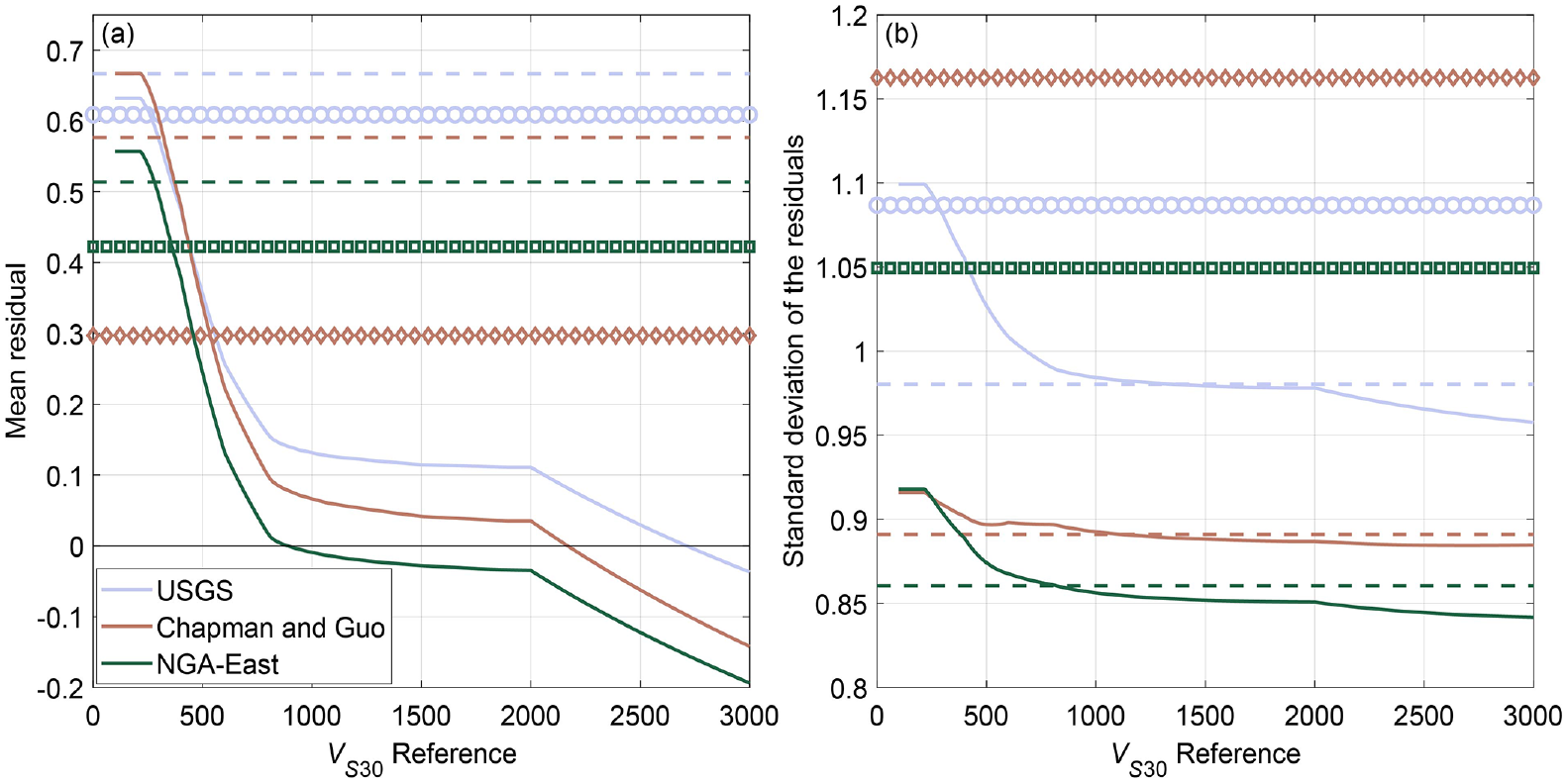
(a) Mean and (b) standard deviation of residuals after application of possible CG21 reference V_S30 values, as specified on the x-axes. Circles (USGS; Thompson et al., 2023), diamonds (Chapman and Guo, 2021), and squares (NGA-East; Goulet et al., 2021b) represent SA_Obs − SA_NGA,3000—no site response or amplification correction; dashed lines—SA_Obs − SA_NGA,3000 − SA_CG(S)—CG21 correction for sediment amplification included; and solid curves—SA_Obs − SA_NGA,3000 − SA_VS30 − SA_CG(S) + cSA_VSref—CG21 sediment amplification, CG21 V_S30 reference condition, and V_S30-based site response included.

Table 1.

Percent decrease in the standard deviation of total residuals at Coastal Plain stations for each model and data set

Data set	Model
	CG21	H L4+N1 mod	H K1 mod	Gea-I	Gea-II
Chapman and Guo	22.7	15.7	14.4	8.0	8.6
NGA-East	16.3	13.3	11	8.9	8.4
USGS	7.1	3.1	5.7	3.8	4.3

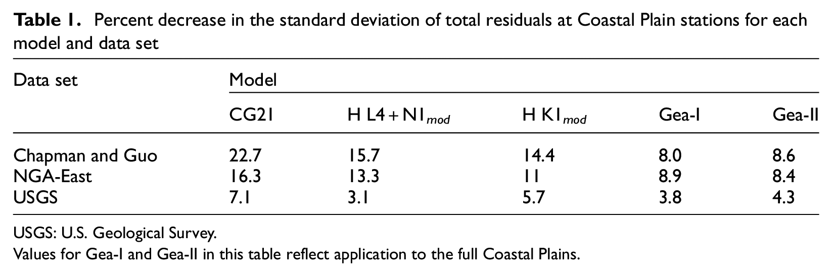
USGS: U.S. Geological Survey.

Values for Gea-I and Gea-II in this table reflect application to the full Coastal Plains.

Other V_S30-based site amplification models could have been used to determine the CG21 reference condition—for example, from GMMs developed for the WUS or previous generations of GMMs developed for the CEUS (Petersen et al., 2015, 2020)—and could yield greater sensitivity to the reference value. But we want to maintain consistency with the 2023 NSHM, which makes use of the model of Stewart et al. (2020). If an improved model becomes available and is applied in future versions of the NSHM, the CG21 reference condition would warrant reevaluation.

Harmon and others

Another potentially applicable set of site amplification models was developed by Harmon et al. (2019a), in which they predict amplification based on sediment thickness and site natural period (T_nat). They defined sediment thickness (Z_Soil) as the thickness of material between the ground surface and a V_S horizon of ∼2000 to 3000 m/s and designate this model L4+N1, where the modular terms correspond to thickness-dependent linear amplification (L4—f(V_S30) + f(Z_Soil)) and nonlinear amplification conditioned on spectral acceleration at a rock site (V_S = 3000 m/s; N1—f(NL)). The site amplification model conditioned on site natural period is designated K1 (f(V_S30) + f(T_nat) + f(NL)).

The formulations for f(V_S30), f(Z_Soil), and f(T_nat) from Harmon et al. (2019a) are as follows:

$$f\left(V_{S30}\right)=\{\begin{array}{c}0\hfill \\ \multicolumn{1}{c}{c_1\ln (V_{S30}/V_c)}\\ \multicolumn{1}{c}{c_1\ln (V_{S30}/V_c)+c_2\ln (V_{S30}/V_L)+c_{3}l{n}^2(V_{S30}/V_L)}\end{array}\begin{array}{c}{V}_{S30}>V_c\hfill \\ V_L<V_{S30}<V_c\hfill \\ V_{S30}<V_L\hfill \end{array}$$

(3)

$$f\left(Z_{\mathrm{Soil}}\right)=\{\begin{array}{c}0\hfill \\ \multicolumn{1}{c}{c_4{(Z_{\mathrm{Soil}}-30m)}^2}\end{array}\begin{array}{c}{Z}_{\mathrm{Soil}}<30m\hfill \\ \multicolumn{1}{c}{Z_{\mathrm{Soil}}\ge 30m}\end{array}$$

(4)

$$f\left(T_{\mathrm{nat}}\right)=\{\begin{array}{c}{c}_6{T}_{\mathrm{nat}}\hfill \\ \multicolumn{1}{c}{c_{5}R+c_6{T}_{\mathrm{nat}}}\end{array}\begin{array}{c}{T}_{\mathrm{OSC}}<0.01\sec \hfill \\ \multicolumn{1}{c}{T_{\mathrm{OSC}}\ge 0.01\sec }\end{array}$$

(5)

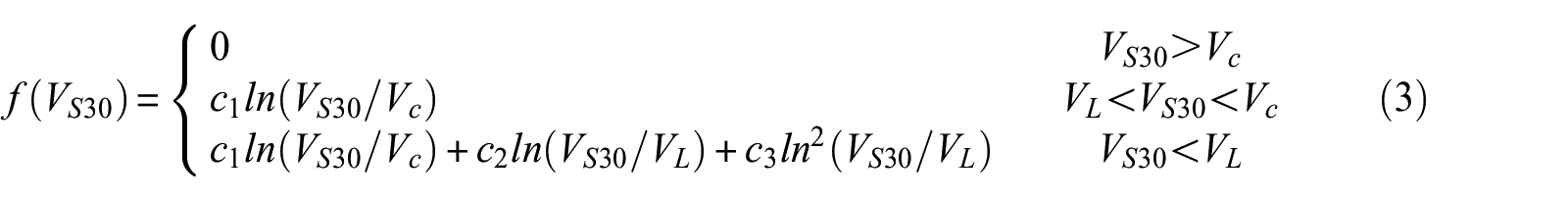
where c₁, c₂, c₃, c₄, c₅, and c₆ are period-dependent coefficients; V_c is the period-dependent velocity bound above which zero amplification occurs relative to a reference condition of V_S = 3000 m/s; V_L is the period-dependent limiting velocity below which amplification does not reduce linearly with increasing V_S30; and T_OSC is the oscillator period. R is a Ricker wavelet term,

$$R=\frac{2}{\sqrt{3\alpha }{\pi }^{\frac{1}{4}}}(1-\frac{{\beta }^2}{{\alpha }^2})\exp (-\frac{{\beta }^2}{2{\alpha }^2}),$$

(6)

where α is the period-dependent regression coefficient, and β is given by

$$\beta =\ln \left(\frac{T_{\mathrm{OSC}}}{T_{\mathrm{nat}}}\right)-\ln (0.81)$$

(7)

In addition, the nonlinear site amplification (N1 or f(NL)) is specified by

$$f\left(\mathrm{NL}\right)=\{\begin{array}{c}{f}_2\ln \left(\frac{I_r+f_3}{f_3}\right)\hfill \\ \multicolumn{1}{c}{0}\end{array}\begin{array}{c}{V}_{S30}<V_c\hfill \\ \multicolumn{1}{c}{V_{S30}\ge V_c}\end{array}$$

(8)

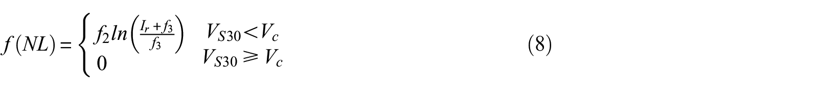
where I_r is the 5% damped pseudo-spectral acceleration at a rock-outcrop condition of V_S = 3000 m/s for N1 and K1 models, f₃ is a period-dependent coefficient, and f₂ is

$$f_2=f_4[\exp \left\{f_5(\min (V_{S30},3000)-360)\right\}-\exp \left\{f_5(3000-360)\right\}],$$

(9)

where f₄ and f₅ are period-dependent coefficients.

The model based on sediment thickness would seem ideal for direct application to the Coastal Plains, but it was derived using profiles having sediments only up to 1 km thick and has a functional form that does not extrapolate well for greater thicknesses due to an amplification that scales with the square of the thickness parameter. We adjust this functionality such that the thickness dependence is square root rather than squared and scale their c₄ coefficient to minimize, through a grid search, the standard deviation of total ground-motion residuals using the Chapman and Guo (2021) data set (Figure 11a). This new model is designated L4+N1 _mod . For the site-natural-period model, we convert Coastal Plain sediment thickness to T_nat using a time-averaged shear-wave velocity profile, which we derive, again, to minimize the standard deviation of total ground-motion residuals using the Chapman and Guo (2021) data set (Figure 11a). We constrain the profile to have an average V_S30 equal to that at the Chapman and Guo (2021) stations, or about 360 m/s, and a shear-wave velocity at the base approaching 3000 m/s. This method is preferred to using existing measured profiles because there are very few deep profiles with which to obtain a Coastal Plain average, and, more importantly, we want to maximize the correlation between observed amplification and the T_nat functionality in Harmon et al. (2019a), which was not optimized for the Coastal Plain. We also use an adjusted version of the c₆(T) coefficients (Supplemental Table S1) for the f(T_nat) term of the site-natural-period model, which was smoothed for periods from 1.0 to 10.0 s, to remove an unrealistic reduction in the predicted spectral amplifications above 1.0-s period that becomes more pronounced with increasing sediment thickness. This model is designated K1 _mod .

Figure 11.

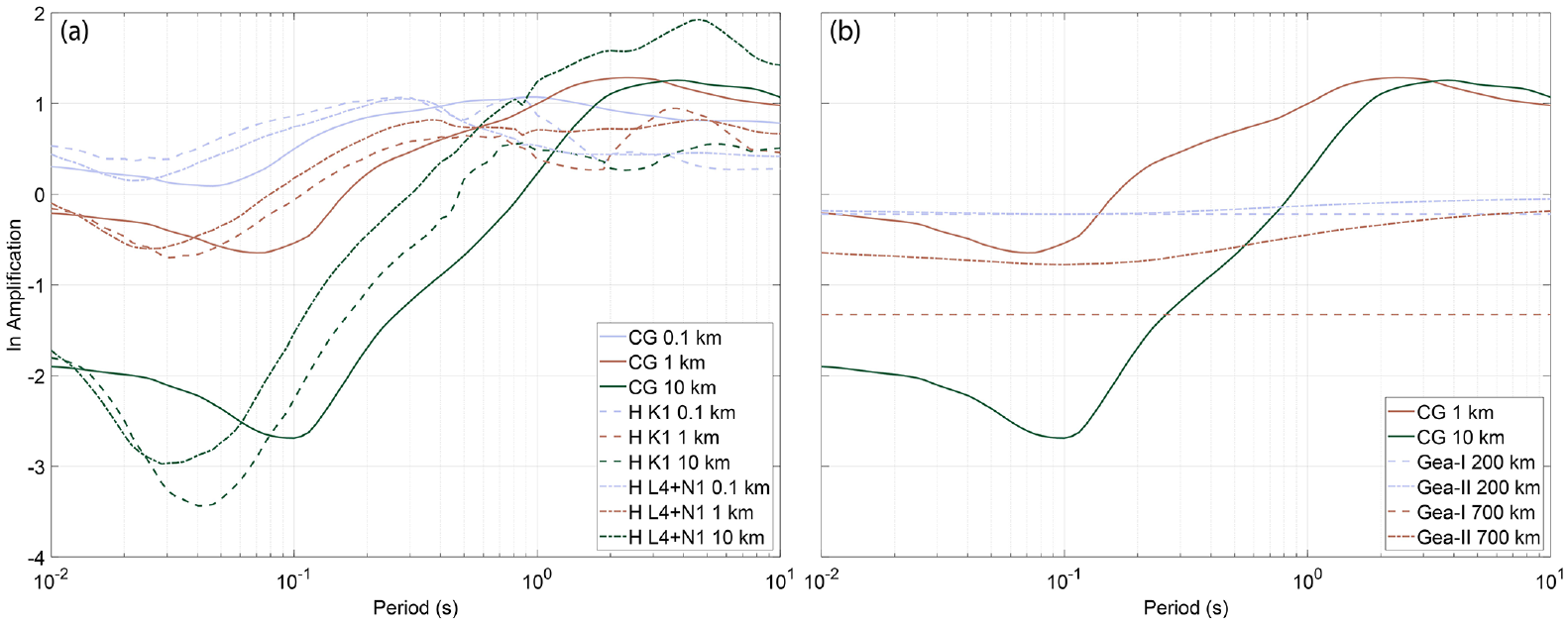
Comparison of the period and sediment thickness dependence of Chapman and Guo (2021; CG) to (a) Harmon et al. (2019a; H) sediment-thickness-based (L4+N1) and site-period-based (K1) models and (b) NGA-East (Goulet et al., 2021a) period-independent (Gea-I) and period-dependent (Gea-II) models. For Harmon et al. (2019a), ground motions are assumed to be linear for an average Coastal Plain site condition with a V_S30 of 350 m/s.

The resulting scaling value of the c₄ coefficient is 2.5 × 10⁴, and the time-averaged velocity profile in m/s has the form 350 + (3000 − 350) × (1 − exp(−h/7.5)), where h is the sediment thickness in km. This time-averaged velocity profile is about 30% slower than the time-averaged profile inferred from the velocity profile published by Cunningham and Lekic (2020) for the Atlantic Coastal Plain, and is similar to that inferred from the profile published by Chapman et al. (2006) for Charleston, South Carolina. The standard deviation of total ground-motion residuals (SA_Obs − SA_NGA,3000 − SA_{L4+N1mod,K1mod}) using the Chapman and Guo (2021) ground-motion data set for periods between 0.1 and 3.0 s, relative to not using the L4+N1 _mod and K1 _mod models, is reduced by 14% and 16%, respectively (Table 1). And like CG21, these models flatten at long periods, leading to residual bias beyond 3.0-s period. The time-averaged velocity profile inferred from Cunningham and Lekic (2020) could be applied in the K1 _mod model, and the reduction in standard deviation of total ground-motion residuals would be reduced slightly, 14% as opposed to 16%. However, the Cunningham and Lekic (2020) profile predicts unreasonably high velocities below about 4 km depth, approaching 7 km/s at 15 km depth, leading to site-natural-periods and ground-motion adjustments that are too small.

NGA-East

We can also consider the Gulf Coast path-attenuation models derived by the NGA-East project (Goulet et al., 2018, 2021a). They derived two models—one period independent (Gea-I) and one period dependent (Gea-II)—in which decreasing ground motions accompany increasing path lengths traversed across the Gulf Coastal Plain as measured along the ground surface. These models are fundamentally different than the CG21 and Harmon models in that the CG21 and Harmon models only account for the effects of sediments vertically beneath the site. Furthermore, both NGA-East models are parameterized as modifications to the anelastic attenuation term of the NGA-East GMMs, and thus by definition only attenuate ground motions, with the period-dependent model attenuating ground motions most at 0.1-s period. For the comparison in Figure 11b, we calculate average Coastal Plain path lengths of 200 and 700 km, which correspond to the NGA-East data set of source–receiver pairs having sediment thicknesses of about 1 and 10 km, respectively. We see that there is a modest correlation between CG21 amplifications and the Gulf Coast adjustment factors. At short periods, increasing sediment thickness and increasing path length are associated with increasing attenuation. At long periods, however, they act in the opposite sense—CG21 amplifications increase with increasing sediment thickness, whereas Gulf Coast adjustment factors attenuate more with increasing path length.

The NGA-East project considered small and large Gulf Coast polygons for application of the adjustment factors (Figure 12). Like the Harmon models, we calculate total ground-motion residuals (SA_Obs − SA_NGA,3000 − SA_VS30 − SA_NGA-East) using the NGA-East data set (Goulet et al., 2021b) to estimate how much Gea-I and Gea-II reduce the standard deviation of total residuals between 0.1- and 3.0-s periods, relative to not using these factors. When path lengths are calculated for each source–receiver pair in the NGA-East data set across the small polygon and we apply Gea-I and Gea-II adjustment factors, the standard deviation of total ground-motion residuals decreases by 3% and 4%, respectively. For the large Gulf Coast polygon, the standard deviation decreases by 10% and 8%, respectively.

Figure 12.

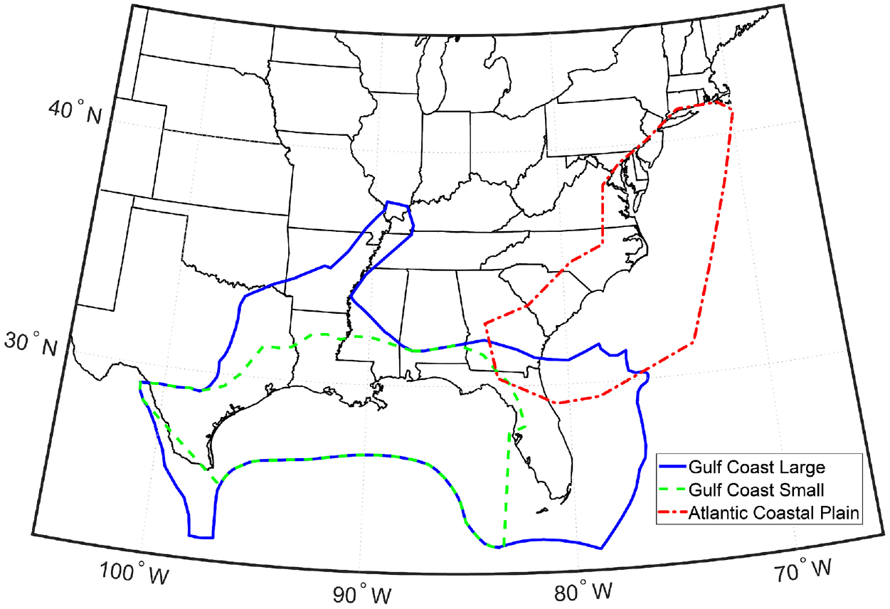
Atlantic and Gulf Coastal Plain polygons used for application of the NGA-East adjustment factors. The Atlantic Coast polygon was drawn as part of this study. The two Gulf Coast polygons are from the work by Goulet et al. (2018).

We also consider application of the adjustment factors for a polygon encompassing the Atlantic Coastal Plain (Figure 12) as well as the entire extent of the Coastal Plains surface shown in Figure 3. For application of the Gea-I and Gea-II adjustment factors to the Atlantic Coastal Plain polygon, the standard deviation of total ground-motion residuals decreases by 0.4% and 3%, respectively, and for the full extent of the Coastal Plains, by 9% and 8%. We note, however, that the NGA-East data set for the Atlantic Coastal Plain is dominated by stations in South Carolina. After the passing of USArray, the station distribution is more uniform (Figure 6b), but we find that the change in standard deviation using the Chapman and Guo (2021) data set with the Atlantic Coastal Plain polygon is similarly low. Using the USGS data set (Thompson et al., 2023), however, standard deviations decrease by 7% and 4%. For paths that fall within the full extent of the Coastal Plains, the standard deviations for Gea-I and Gea-II decrease by 8% and 9% using the Chapman and Guo data set, and by 4% using the USGS data set (Table 1). Although the spectral accelerations are very similar between data sets within the range of periods considered for this analysis, differences in how well models can account for ground motions and reduce standard deviations arise due to differing magnitude estimates for a given earthquake and differing source and receiver distributions.

Potential implementation in the USGS NSHM

Based on the above analyses, we recommend a logic-tree approach to incorporate the aforementioned models into the USGS NSHM. Because all three attenuation and amplification models considered in this article reduce the standard deviation of total residuals for all three independent data sets (Table 1), indicating a better fit to the data, a basic logic tree could include the three models with weights proportional to their ability to reduce the standard deviation of residuals (Figure 13): the CG21 model with a weight of 0.5; L4+N1 _mod ,K1 _mod —0.25; and Gea-I,II—0.25—with path lengths calculated for the full extent of the Coastal Plains where all three data sets exhibit a reduction in the standard deviation of residuals. Furthermore, the logic tree could consider uncertainty in sediment thickness, with a weight of 0.5 on the map presented in Figure 3, and weights of 0.25 on those thicknesses multiplied and divided by 1.2, which represents a distribution slightly larger than that corresponding to the reported uncertainty of sediment thickness.

Figure 13.

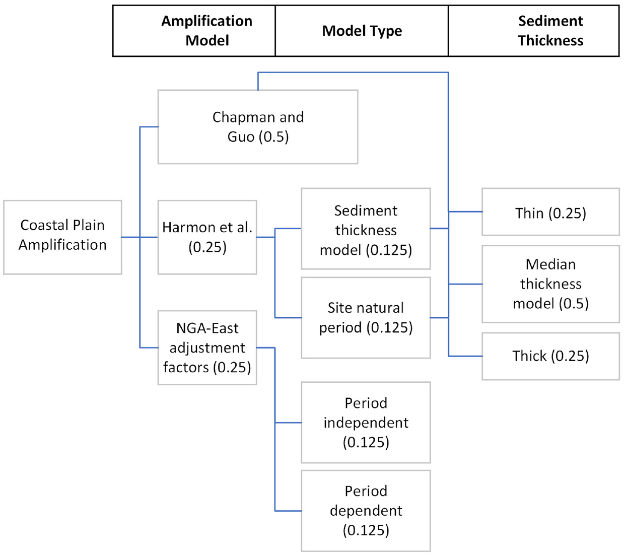
Proposed logic tree to incorporate Coastal Plain attenuation and amplification models.

In this work, we do not distinguish whether earthquakes contributing to anomalous ground motions in the Coastal Plains occur inside or outside the Coastal Plain or in regions where human activities have potentially induced earthquakes such as in Texas, Oklahoma, and Kansas (Zalachoris and Rathje, 2019). For example, Guo and Chapman (2019) found that ground motions observed at non-Coastal Plain stations from earthquakes within the Coastal Plain were similarly anomalous to observations at Coastal Plain stations from earthquakes outside the Coastal Plain. Regarding potentially induced earthquakes, Ramos-Sepulveda et al. (2023) found that earthquakes occurring in Texas, Oklahoma, and Kansas had more negative short-period high-frequency ground-motion residuals relative to earthquakes occurring elsewhere in the CEUS, and Shahjouei and Pezeshk (2016) excluded potentially induced earthquakes from their ground-motion modeling efforts in the CEUS due to the possibility of anomalous ground motions (Hough, 2014).

Future efforts to improve seismic hazards assessments in the USGS NSHM Coastal Plain region could involve the direct application of GMMs developed specifically for this area (e.g. Pezeshk et al., 2021). Future areas of research could build on this work to improve characterization of earthquake ground motions on the Coastal Plains. Ground-motion attenuation and amplification models can include better incorporation of strong period-dependent resonances that are observed at locations over thin layers of sediments near the edge of the Coastal Plains (Pratt and Schleicher, 2021). Studies could investigate the effects of soil nonlinearity and magnitude dependence of ground motions specific to the sediments and crustal basement within the Coastal Plains (Zhang et al., 2005). Models could also consider the effects of greater spatial variability in subsurface geology, for example, by including the numerous Mesozoic rift basins beneath the Atlantic Coastal Plains (Withjack et al., 1998) or the many salt domes intruding the Gulf Coastal Plain sediments (Beckman and Williamson, 1990; Torres, 2012).

Conclusion

Observed earthquake ground motions in the Atlantic and Gulf Coastal Plains have a strong period and sediment thickness dependence that cannot be accounted for by the current CEUS V_S30-scaling-model that is implemented in the 2018 USGS NSHM. We compile a sediment thickness map with which we can apply available ground-motion attenuation and amplification models applicable to the thick sediments beneath the Coastal Plains. Assuring a seamless transition to the NSHM in the continental interior and effective application of existing models required additional model development, including a CG21 transitional scaling function, estimation of a CG21 reference condition, reformulation of the Harmon et al. (2019a) sediment-thickness-based model, and coefficient adjustment and development of a velocity profile for the Harmon et al. (2019a) site-natural-period-based model. These models, including those based on the length of path traversed within the Coastal Plains (Goulet et al., 2021a), reduce the standard deviation of total ground-motion residuals by over 20%, and together with the uncertainty in the depth to the syn- and post-rift unconformity, can be combined in a logic tree that could better account for short-period attenuation and long-period amplification of ground motions in future USGS NSHMs.

Supplemental Material

sj-docx-1-eqs-10.1177_87552930231204880 – Supplemental material for Sediment thickness map of United States Atlantic and Gulf Coastal Plain Strata, and their influence on earthquake ground motions

Supplemental material, sj-docx-1-eqs-10.1177_87552930231204880 for Sediment thickness map of United States Atlantic and Gulf Coastal Plain Strata, and their influence on earthquake ground motions by Oliver S Boyd, David Churchwell, Morgan P Moschetti, Eric M Thompson, Martin C Chapman, Okan Ilhan, Thomas L Pratt, Sean K Ahdi and Sanaz Rezaeian in Earthquake Spectra