Estimation of historical earthquake-induced liquefaction in Fraser River delta using NBCC 2020 GMPEs in deterministic and probabilistic frameworks

Abstract

Paleo-liquefaction features of sand dykes and sand blows were identified in the 1990s at multiple host sediments in the Fraser River delta in southern British Columbia all younger than 3500 BP. These paleo-liquefaction sites could be linked to Cascadia subduction earthquakes. Empirical magnitude-bound relationships are often used to estimate paleo-earthquake magnitudes. To determine the lower bound magnitude of Cascadia interface earthquakes that could have generated the paleo-liquefaction features, we use ground motion prediction equations for interface earthquakes from the sixth Canadian seismic hazard model of the 2020 National Building Code of Canada. We estimate the minimum M and its peak ground acceleration (a_max) of an interface earthquake required to initiate paleo-liquefaction in the study region. Starting with three full-rupture deterministic scenarios of varying source-to-site distance, we determine the minimum M required from Cascadia subduction zone interface mega-thrust earthquakes to induce liquefaction in the Fraser River delta spans 8.0–8.9 with a corresponding a_max range of 0.09–0.13g. We also perform a back-calculation paleo-liquefaction analysis in a probabilistic framework to incorporate aleatory uncertainties (cone penetration resistance, groundwater table, and a_max) and epistemic uncertainties (liquefaction simplified model) via the Monte Carlo simulation. The developed probabilistic methodology is also applicable to a forward liquefaction assessment and other liquefaction sites globally. The median M from this probabilistic paleo-liquefaction for the four investigated sites lies between 8.8 and 9.0. Our probabilistic results also reveal that Cascadia interface earthquakes with M > 8.9 lead to a 31%–57% probability of liquefaction triggering in the Fraser River delta. In addition, we developed deterministic and probabilistic magnitude-bound curves specific to Cascadia interface earthquakes and representative site class E conditions. These curves provide more accurate magnitude estimations for predicting seismic-induced liquefaction from Cascadia interface earthquakes for sites in the Pacific Northwest than empirical bound curves.

Introduction

Paleo-liquefaction studies help us expand our understanding of prehistorical earthquakes. Thereby, they improve our insight into the present and future seismic hazards. Large magnitude interface earthquakes of the Cascadia subduction zone have a return period of ~500–600 years in northern Cascadia (Goldfinger et al., 2012; Leonard et al., 2010), much longer than the ~130 year duration of recorded seismicity in southwest British Columbia. This problem leads to the insufficiency of the earthquake catalog for the input parameters of seismic hazard analysis. A paleo-liquefaction investigation can overcome this deficiency to some extent. The lower bound earthquake magnitude and ground motion to induce liquefaction can be estimated from paleo-liquefaction evidence (Green et al., 2005). An earthquake magnitude of as low as 4.5 can trigger liquefaction (Green and Bommer, 2019). Documented liquefaction observations in regions of Christchurch, New Zealand, during the 2010–2011 Canterbury earthquake sequence demonstrated that sand blows can form from earthquakes of M 5.2–7.1 and magnitude normalized to M 7.5 maximum ground accelerations (a_max)_7.5 ≥ 0.06g (Quigley et al., 2013). The Fraser River delta in southern Vancouver, British Columbia, is located at the northern end of the Cascadia subduction zone which causes seismicity in the overriding North American plate, the subducting Juan de Fuca plate, and on the interface between the two plates. There are 12 known paleo-liquefaction sites in Greater Vancouver that are younger than 3500 years old with two sites constrained to younger than 1700 years ago documented by Clague et al. (1992, 1997, 1998) who reported liquefaction features as sand blows, dykes, and sills. They concluded that a large earthquake centered in the Cascadia subduction zone or a crustal earthquake with an epicenter close to Vancouver could be the causative source of liquefaction in the region. Their work could not rule out either a plate-boundary or a crustal event. Turbidite evidence determines eight or five full or near-full Cascadia interface earthquake ruptures in the last 3500 or 1700 years, respectively (Goldfinger et al., 2012; Leonard et al., 2010). Since the paleo-liquefaction features are not as repetitive as great Cascadia interface earthquake ruptures, Clague et al. (1998) concluded that a nearby crustal event is more likely to have generated the paleo-liquefaction features.

The correlation between earthquake magnitude and the most distal liquefaction site from the plausible seismic source is called the magnitude-bound method (Ambraseys, 1988). This procedure is the first approach introduced to estimate the minimum required magnitude to initiate liquefaction from observation of the most distal liquefaction site from worldwide empirical earthquake data. Two different source-to-site distance measures, epicentral distance and distance to the fault, were included in Ambraseys’ data. This relationship was developed based on the assumption that ground motion from an earthquake cannot trigger liquefaction farther than a specific distance. Magnitude-bound curves have been proposed from either global or regional earthquakes data by Papadopoulos and Lefkopoulos (1993), Galli (2000), Papathanassiou et al. (2005), Castilla and Audemard (2007), and Pirrotta et al. (2007). These curves constrain the minimum magnitude of historical earthquakes to have induced the observed paleo-liquefaction events. Other quantitative techniques were developed to define the magnitude of the causative paleo-earthquake and constrain its source location. These quantitative methods were established based on various liquefaction analysis techniques, including the cyclic stress procedure introduced by Seed and Idriss (1971), the strain-based approach of Dobry et al. (1982), and the energy-based method proposed by Green (2001) and Green and Mitchell (2004). In an inverse analysis, the source of liquefaction was determined from the critical strata by setting the factor of safety (FS) against liquefaction to 1. Then, a back-calculation technique estimates the likely combination of moment magnitude (M) and peak ground acceleration (a_max) required to induce liquefaction at the individual site. For some seismically active regions, Obermeier et al. (2001), Olson et al. (2005), and Green et al. (2005) have applied the back-calculation of paleo-liquefaction investigations. Obermeier and Dickenson (2000) back-calculated a_max along the banks of islands in the Columbia River of Oregon and Washington for the 1700 Cascadia subduction earthquake. Their estimation of a_max was as low as 20% of those predicted by recent M 9 simulations (Rasanen et al., 2021). They used hand-held dynamic cone penetrometer measurements rather than standard penetration test (SPT) or cone penetration test (CPT) measurements. Olson et al. (2005) regenerated a regional magnitude-bound relation from the deterministic form of the cyclic stress method for paleo-liquefaction sites in the Wabash Valley in the American mid-west. Gheibi and Gassman (2016) estimated the minimum M–a_max combination of an earthquake dated back to 11,000 years ago to have induced liquefaction at a site in the South Carolina Coastal Plain, USA. They also examined the effect of earthquake age on soil resistance and the associated magnitude estimation. Yousuf et al. (2021) used back-calculation methods based on the cyclic stress procedure to determine the likely minimum magnitude and peak ground acceleration of paleo-liquefaction that occurred in the Kashmir Basin, India. All of these studies predicted M from the deterministic back-calculation analyses of liquefaction features. The deterministic assessment addresses and reduces some of the uncertainties related to the back-calculated methodology and the selection of representative soil resistance. Despite all the described advancements, paleo-liquefaction evaluation still has a large number of uncertainties including aleatory (variabilities in data) and epistemic (uncertainties inherent to the methodology). Strategies used to represent soil characteristics and the groundwater table (GWT) at the time of the earthquake occurrence from existing in situ testing and boreholes rely on qualitative suggestions by Obermeier et al. (2005) which may result in producing additional uncertainties in the back-calculation analyses. Rodriguez-Marek and Ciani (2008) were the first to incorporate uncertainties of model and parameter into paleo-liquefaction assessment using the probabilistic SPT-based liquefaction analysis method of Cetin et al. (2004) for one site in South Carolina Coastal Plain near the cities of Charleston and Georgetown, USA. However, the uncertainties in soil resistance and the location of groundwater at the time of the earthquake were neglected in their study. Maurer et al. (2015) proposed a probabilistic framework to develop magnitude-bound relations for New Zealand. They presented their new methodology for shallow crustal earthquakes.

This study reviews the paleo-liquefaction features in Greater Vancouver and uses nearby in situ CPT and SPT testing to select representative soil parameters for four paleo-liquefaction sites. We first back-calculate the minimum M and a_max of a Cascadia interface earthquake to trigger liquefaction features in the Fraser River delta region using a simplified deterministic framework in which M and a_max are determined using ground motion prediction equations (GMPEs) of the sixth national seismic hazard model of the 2020 National Building Code of Canada (NBCC). We also evaluate liquefaction features via probabilistic methodologies by incorporating uncertainty of SPT- and CPT-based liquefaction analysis methods. Uncertainties associated with soil characterization, groundwater depth, and ground motion variabilities are also incorporated into our probabilistic paleo-liquefaction analysis framework. A novel probabilistic approach is adopted to account for uncertainties in parameters and Boulanger and Idriss’ (2014) CPT-based method via the Monte Carlo simulation. The proposed methodology is not limited to backward analysis but also can be applied to a forward probabilistic analysis. This study constrains the minimum M of a Cascadia interface earthquake to induce liquefaction in the Fraser River delta given in situ site conditions and current treatment of the seismic demand. In the final section of this article, magnitude-bound curves are developed for Cascadia interface earthquakes within deterministic and probabilistic frameworks. We suggest using these curves for Pacific Northwest paleo-liquefaction sites affected by the Cascadia subduction zone rather than empirical bound curves of Ambraseys (1988) or others.

Paleo-liquefaction features in Fraser River delta

In this section, we provide a brief description of the paleo-liquefaction evidence found in the study area. Clague et al. (1992) documented sand blows, sand dykes, and sills in the Fraser River delta and near the Serpentine River floodplain in southwestern British Columbia. Sand dykes are sedimentary injections that cut through soil beddings, while sand sills are injected parallel to the bedding. Sand blows or sand boils are a volume of sand vented onto the paleo-ground surface (Clague et al., 1992). In total, 12 paleo-liquefaction sites were identified in building excavation sites and beside riverbanks in the region (Clague et al., 1998). Figure 1 shows the geology map of the Fraser River delta with the scattered locations of the 12 known paleo-liquefaction sites. Four sites are located in the Serpentine River floodplain in the southeast of the map area, while the remaining sites are located primarily in the center but also east and south of the Fraser River delta. The delta formed following the retreat of the last ice sheet around 13,000–11,000 years ago (Clague et al., 1983). The upper geology unit (unit 1) consists of a floodplain, intertidal silts, and silty sands of 3–15 m thick and peat of up to 8 m thick. Unit 1 overlies unit 2 which is a poorly graded, fine-to-medium sand with a variable thickness of 10–20 m. This unit is believed to be the source of paleo-liquefaction features discovered in the region (Clague et al., 1992, 1997; Naesgaard et al., 1992). Generally, the sand layer below the clay and silt cap with low normalized cone resistance could be the plausible source of liquefaction.

Figure 1.

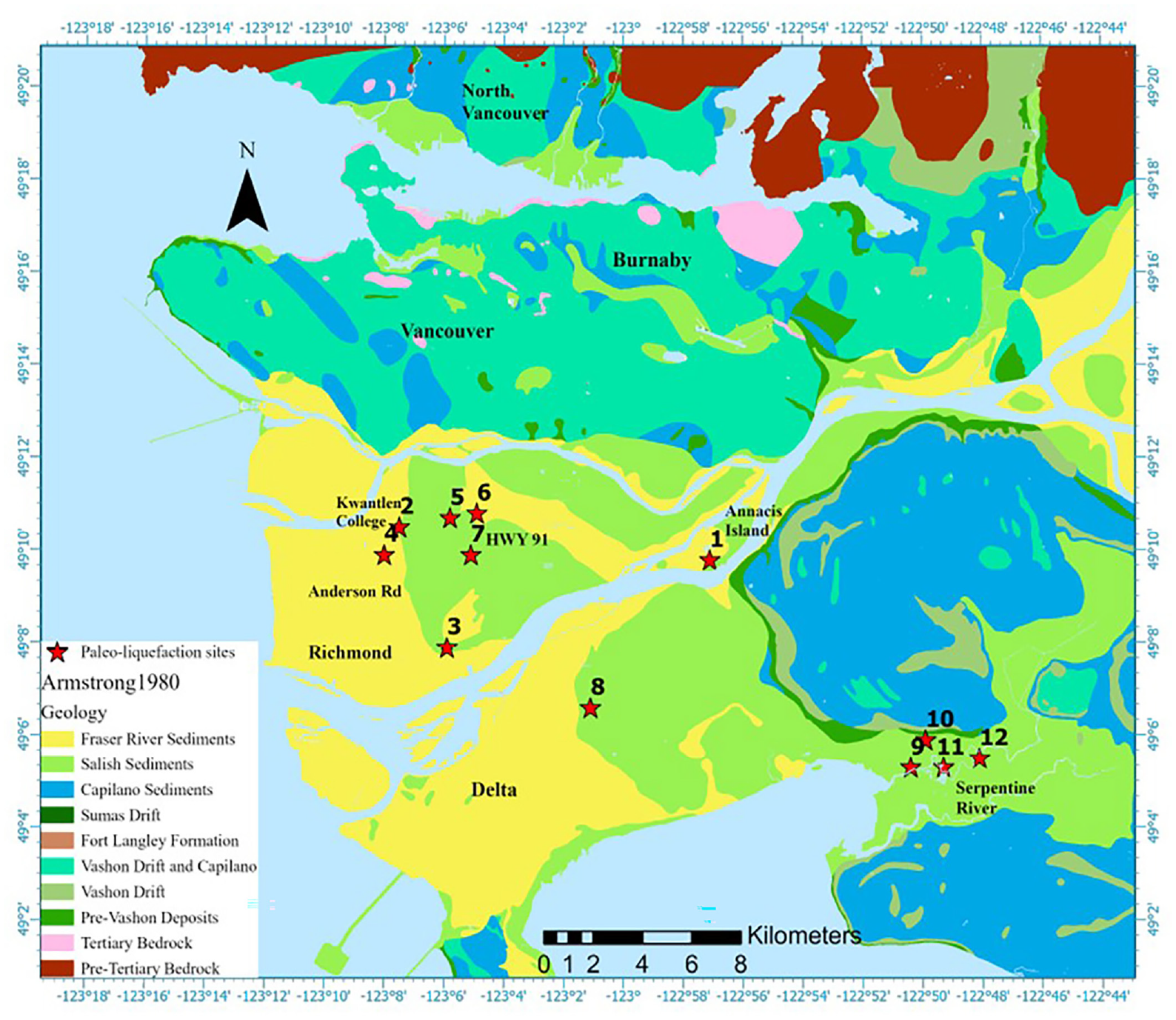
Geology map of Greater Vancouver showing locations (red stars) of 12 paleo-liquefaction sites of Clague et al. (1998).

This study will assess paleo-liquefaction at sites 1–4. Site 1 in Southwestern Annacis Island has large sand blows and numerous sand dykes with thicknesses varying from a few millimeters to about 25 cm. These features were exposed in the wall of an excavation in 1996 (Clague et al., 1997). Soil stratigraphy shows 2.5–3.0 m of a fill mostly composed of sand overlying a 20-cm thick, brown, organic-rich soil. Underlying the fill material is a clayey silt unit of 3.0–5.5 m thick. Large sand blows and sand dykes were observed within these clayey silt layers and at the soil surface. The vented sand has a similar texture to sand unit 2. Therefore, the liquefiable layer is potentially the thick sand unit 2 below the base of the excavation. Site 2 in the northern-central area of the Fraser River delta nearby Kwantlen College includes many sand dykes and sand blows observed in the excavation wall. Soil stratigraphy at this site contains 2–3 m of a silty clay upper unit (unit 1) overlying 20–30 m of a uniformly graded fine-to-medium sand with some silt. The sand dykes have thicknesses varying from less than a millimeter to around 30 cm (Clague et al., 1998). In some profiles, sand dykes have exuded to the ground surface by forming sand blows. The grain size distribution of these dykes is similar to samples from sand unit 2 (Naesgaard et al., 1992). Hence, unit 2 could be the source of liquefaction features. The sand unit has cone penetration resistance (q_c) ranging from 1.7 to 13 MPa (Clague et al., 1992). Sand blows and sand dykes with a maximum thickness of 5 mm were reported at site 3, south of the city of Richmond (Clague et al., 1998). Sand dykes cut through the upper layer and vented onto the ground surface as a result of sand boiling at this site. The nearby CPT profile shows sand layers with q_c values ranging from 1.5 to 13 MPa (Clague et al., 1992), which are susceptible to liquefaction. Accordingly, these sand layers could be the source of liquefaction. Site 4 in the center of Richmond near Anderson Road contains a 12-mm wide sand dyke observed in a piston core taken at a depth of 2 m (Clague et al., 1992). The soil profile consists of about 3 m of mud (top), 2.5 m of very loose silty fine sand, and 10.5 m of medium sand. The loose continuous sand layer with low cone tip resistance (Clague et al., 1992) is believed to be the source of liquefaction. The selected liquefaction sources for these four sites are the sand sublayers with low cone tip resistance. Sites 5–7 are in the Richmond area along Highways 99 and 91 and had several sand dykes and sills. Site 8 in the Burns bog area of Delta and sites 9–12 within the Serpentine River’s floodplain all exhibit sand dykes and sills with the exception of one Serpentine River site that had a silty dyke. All liquefaction features are dated to be younger than ca. 3500 BP and some are younger than 2400 BP (Clague et al., 1998). Site 1 was dated back to 1763 (±42) C14 years BP or about 1700 years ago (Clague et al., 1997, 1998).

Clague et al. (1997) suggested that a crustal earthquake or strong plate-boundary earthquake in the Cascadia subduction zone could be responsible for the liquefaction features found in this region. Clague et al. (1997, 1998) examined the probability of liquefaction using the third national seismic hazard model (associated with the 1985 NBCC) and an available southwest BC seismic hazard model of BC Hydro but neither model included the Cascadia subduction zone’s interface earthquake source. They also estimated a magnitude 8 or higher earthquake from Ambraseys’ (1988) correlation considering the Cascadia subduction zone as the plausible source. We do not repeat their effort to identify which source type led to the paleo-liquefaction features, driven primarily by the continued significant uncertainty in crustal earthquake source parameters (magnitude, hypocenter location) in southwest British Columbia. Rather, we focus on constraining the M and a_max of Cascadia interface earthquakes to induce liquefaction given updated knowledge of their seismic demand, measurements of the local soil resistance, and using a probabilistic framework to include uncertainties. We note that there is increasing evidence of recently active crustal faults in southwest British Columbia (e.g. Harrichhausen et al., 2022; Kelsey et al., 2012; Morell et al., 2018) to re-evaluate in future whether crustal sources may have induced these paleo-liquefaction features. Future work is required to address shallow crustal earthquake sources given updated GMPEs, the ongoing identification of active crustal faults (e.g. newly identified Elk Lake fault (unpublished) that possibly connects with the Central Haro Strait fault) as well as the possibility that unknown (buried) faults may be present beneath the deep Fraser River delta (e.g. Bastin et al., 2016). We examine the possibility of the Cascadia subduction zone being a causative earthquake source for liquefaction features in the Fraser River delta using regional interface-source GMPEs of the sixth national seismic hazard model (associated with the 2020 NBCC). We further investigate this hypothesis via deterministic, and for the first time probabilistic, back-calculation analyses. The inverse computations provide estimations of the earthquake magnitude and peak ground acceleration of Cascadia interface earthquakes to induce the observed paleo-liquefaction.

Selecting representative soil characterization

In this section, we provide a procedure to select representative soil parameters and GWT estimation at the time of the earthquake for each paleo-liquefaction site. We compiled available in situ testing results from the Metro Vancouver seismic microzonation mapping project’s geodatabase (Adhikari et al., 2021; Molnar et al., 2020) and Clague et al. (1997, 1998), including borehole logs, two SPT, and four CPT data nearby paleo-liquefaction sites 1–4. These in situ tests are close enough to the site to represent reasonable soil properties for the source of liquefaction features. Note that we did not have in situ measurements for other paleo-sites.

To distinguish the liquefiable layers from non-liquefiable layers, we considered soil layers below the GWT in combination with soil behavior type indices (I_c) from adjacent boreholes based on Robertson and Cabal (2015). In our study, if I_c was greater than 2.60, then the soil was considered too clayey to liquefy. We corrected the cone tip resistance (q_c) and the number of SPT blow counts (N₆₀) for overburden stress by applying the overburden stress correction factor (C_N) proposed by Boulanger (2003). Equivalent clean sand SPT and CPT resistances were determined by applying adjustments for the effect of fines content (FC) on these penetration resistances following empirical correlations proposed by Boulanger and Idriss (2012, 2014). For SPT sites, we obtained FC from the associated lithology logs. The overburden stress normalized cone tip resistance q_c1Ncs is presented as a dimensionless number by a further normalization with respect to a reference pressure of P_a = 100 kPa. We select representative values of q_c1Ncs (overburden stress normalized clean sand equivalent cone tip resistance) and (N₁)_60cs (overburden stress normalized clean sand equivalent SPT blow count) from the layer that is most susceptible to liquefaction for each paleo-liquefaction site. First, we should identify the critical layer. One method is calculating cyclic resistance ratio (CRR) and considering the continuous layers with lowest CRR as the critical strata. Such a method is suggested by Moss et al. (2006) where multiple critical layers may exist. To determine the critical layer, an earthquake scenario (M = 7.5 and a_max = 0.3 g) is required to calculate the FS against liquefaction. We used the latest CPT- and SPT-based methodology by Boulanger and Idriss (2012, 2014) to define the critical layers. We should note that there is no clear statement of what the critical layer is, and a great deal of judgment is inherent in selecting the critical layers (Green and Olson, 2015). The selection and properties of critical layers can vary with different simplified methods. In this study, the critical layer was defined as the layer with minimum continuous FS less than 1. To consider the soil condition during a paleo-earthquake event, we removed the fill material and estimated the GWT at the time of the liquefaction occurrence. The present GWTs within the study region are shallow, ranging from 1.5 to 3.2 m below the ground surface. Obermeier et al. (2005) suggested that when a fine-grained cap was underlain by liquefiable sand layers, the water table at the time of an earthquake occurrence could be at or above the cap layer. Based on the observed liquefaction features from our sites and following the suggestions of Obermeier et al. (2005), we considered the GWT within the cap layer (silt and clay) and close to the ground surface. Clague et al. (1997) estimated the GWT at the time of the earthquake only for site 1, which is close to our estimation.

Figures 2 and 3 show q_c1Ncs, (N₁)_60cs, and FS profiles as well as the identified critical soil layer for paleo-liquefaction sites 1 and 2. Figure 11 in Appendix 1 shows the profiles and critical layer identification specific to sites 3 and 4. For site 1, the CPT resistance indicates a plausible source of liquefaction at a depth of 6.10–17.50 m with an average q_c1Ncs = 104. The critical strata from SPT resistance for this site lie at a depth of 6.05–15.55 m with an (N₁)_60cs = 14. For site 2, the CPT results indicated a continuous critical layer at a depth of 3.40–19.85 m below the ground surface with an average q_c1Ncs = 97. We also selected a critical layer from SPT profile for site 2 at a depth of 3.40–18.20 m with an average (N₁)_60cs = 17. For sites 1 and 2, the critical sublayer corresponds to sand deposits with average FC of 5% and 12%, respectively. For sites 3, the critical sublayers are located at depths of 3.70–7.55 m and 9.10–20.0 m. These two critical layers have an average q_c1Ncs = 100 and 82, respectively. The critical layer for site 4 is at a depth of 5.40–14.10 m with an average q_c1Ncs = 116. The average FC over the critical silty sand layers for sites 3 and 4 was 12% and 3%, respectively.

Figure 2.

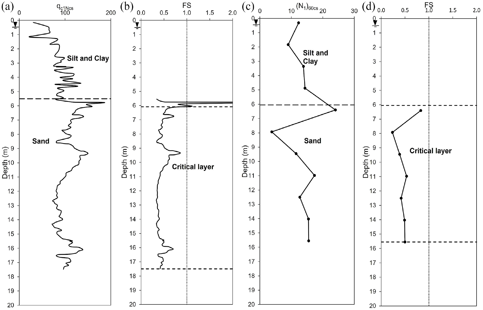
Critical layer identification for site 1 from nearby (a) CPT and (c) SPT measurements and the corresponding calculation of FS (b and d, respectively).

Figure 3.

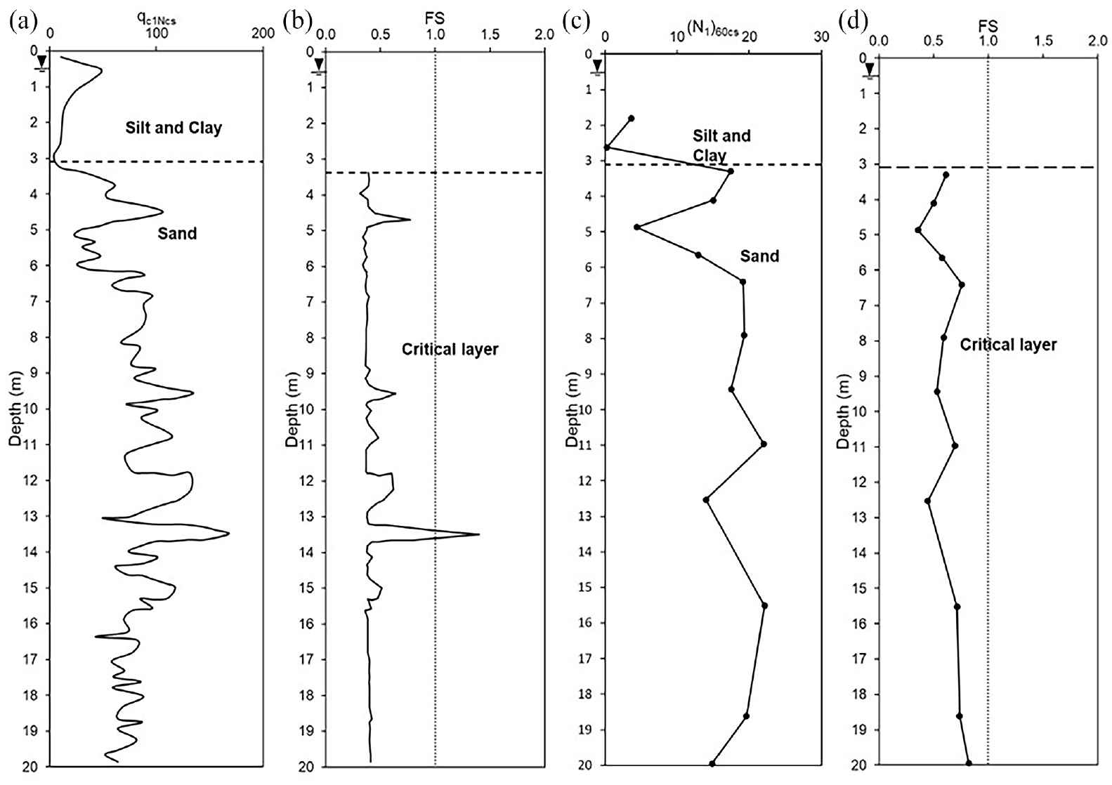
Critical layer identification for site 2 from nearby (a) CPT and (c) SPT measurements and the corresponding calculation of FS (b and d, respectively).

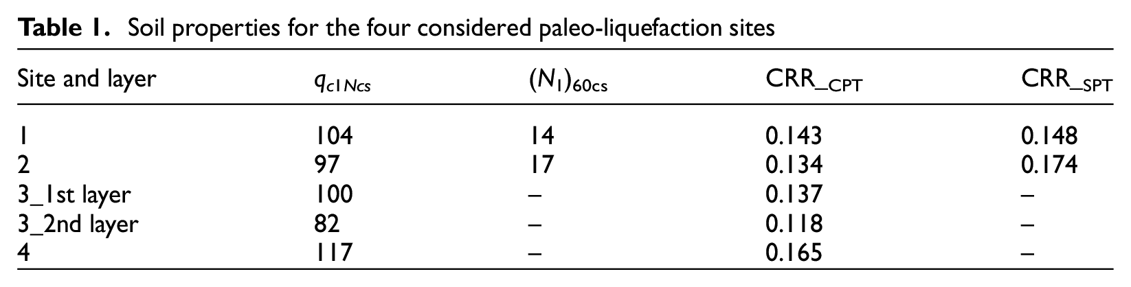
CRRs used in defining the critical layers were calculated from the SPT- and CPT-based liquefaction analyses methods proposed by Boulanger and Idriss (2012, 2014). Table 1 shows the average q_c1Ncs and (N₁)_60cs and the corresponding CRR values within the critical layers at each site. We used these selected soil representative parameters to estimate minimum M and the minimum peak ground acceleration to induce liquefaction in a deterministic framework. We then proceed to estimate the minimum M using a probabilistic methodology considering uncertainties.

Table 1.

Soil properties for the four considered paleo-liquefaction sites

Site and layer	qc 1Ncs	(N1)60cs	CRR_CPT	CRR_SPT
1	104	14	0.143	0.148
2	97	17	0.134	0.174
3_1st layer	100	–	0.137	–
3_2nd layer	82	–	0.118	–
4	117	–	0.165	–

Deterministic estimation of M and a_max

As described earlier, there are available empirical magnitude-bound curves which can provide the minimum earthquake magnitude for the most distal liquefaction sites. However, we were limited in employing available empirical magnitude-bound curves that satisfy our criteria: (1) developed based on distance from the fault, (2) extended to magnitudes greater than 8, and (3) applicable to worldwide earthquakes. Figure 4 shows two magnitude-bound curves proposed by Ambraseys (1988) and Papadopoulos and Lefkopoulos (1993). These empirical curves were formulated based on liquefaction observations from worldwide earthquakes. We also show the distance of site 1 from the Cascadia fault on Figure 4; the distance of all paleo-liquefaction sites in Metro Vancouver lies within the plotted thickness of this distance line. 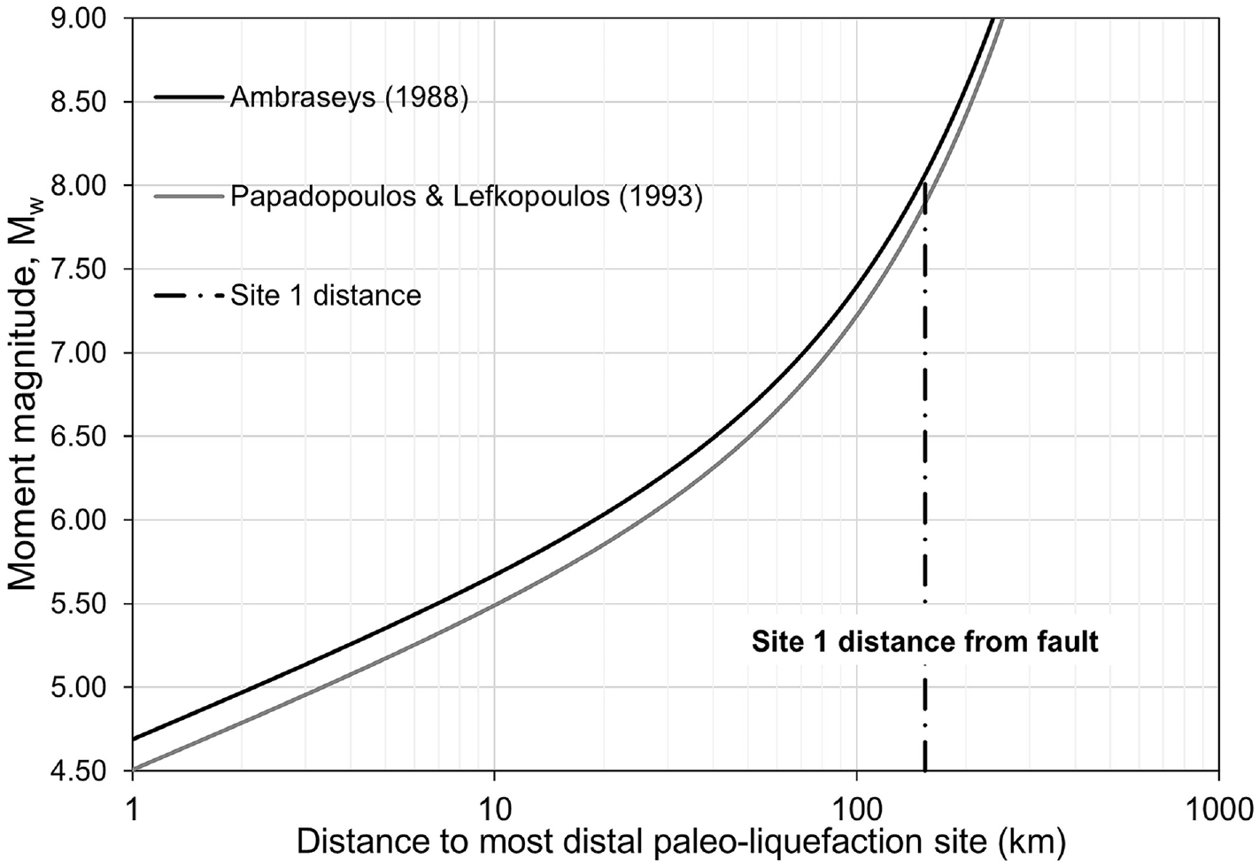For site 1, Ambraseys (1988) and Papadopoulos and Lefkopoulos (1993) provide minimum M of 8.0 and 7.9, respectively. These empirical curves provide the lower bound M for liquefaction occurrence at site 1. As the majority of cases used by Ambraseys were from shallow crustal earthquakes, the application of these curves for the Cascadia fault could result in significant errors. The earthquake characteristics and soil parameters vary regionally, so site-specific correlations could provide more accurate estimates of the minimum earthquake magnitude than that determined from Ambraseys curves or other similar empirical methods. For earthquakes with large return periods such as Cascadia interface events, a back-calculation methodology using region and source specific GMPE(s) is needed.

Figure 4.

Magnitude-bound curves in terms of distance to fault by Ambraseys (1988) and Papadopoulos and Lefkopoulos (1993) to determine the lower bound M for paleo-liquefaction at site 1.

We proceed to use the soil engineering properties of the liquefaction source layers to perform a deterministic backward analysis to estimate lower bounds on the M and a_max to induce liquefaction by a Cascadia interface earthquake. To apply the back-calculation procedure of Green et al. (2005) at our four selected paleo-liquefaction sites, we identified the critical layer responsible for liquefaction features. It is assumed that the source layers of liquefaction had an FS = CRR/CSR₁, _{M= 7.5} = 1. CSR is the cyclic stress ratio applied by an earthquake which is calculated following the simplified stress-based liquefaction analysis. The FS equal to or less than one implies that liquefaction will be induced. We estimate the minimum a_max at the ground surface required to induce liquefaction from the Green et al. (2005) back-calculation technique:

$$a_{\max }=\mathrm{CRR}\mathrm{MSF}{k}_{\sigma }\frac{g{\sigma }_{v0}\prime }{0.65{\sigma }_{v0}{r}_d}$$

(1)

where a_max is the maximum acceleration applied by the earthquake, MSF is the magnitude scaling factor (Boulanger and Idriss, 2014), k_σ is an effective overburden stress correction factor, σ_v is the total vertical stress, and r_d is a stress reduction factor. CRR was calculated from the individual CPT and SPT profiles for the four paleo-liquefaction sites.

The above procedure delineates the boundary of M–a_max combinations that can initiate liquefaction from those that cannot. Thus, we have a wide range of M–a_max combinations to induce liquefaction (see Figure 5). To establish the M–a_max range at which potential Cascadia interface earthquakes would induce liquefaction, we apply applicable GMPE(s). We employed the four interface-source GMPEs of the sixth Canadian national seismic hazard model (Kolaj et al., 2019), including Abrahamson et al. (2016), Atkinson and Macias (2009), Ghofrani and Atkinson (2014), and Zhao et al. (2006). Our study is the first to use the suite of interface GMPEs of the 2020 NBCC in a paleo-liquefaction evaluation. The applicable M range of the interface GMPEs is between 7 and 9.25. The GMPE consists of a median prediction and a measure of the uncertainty introduced by a standard deviation of the model. In the deterministic back-calculation, we only used the median a_max, whereas in the probabilistic framework, we also included the standard deviation of each GMPE model. We use the 2020 NBCC weighting factors of 0.25 for each of the four GMPEs in our analyses to determine the mean a_max for each tested M (0.1 M increment between 7 and 9). Equal weighting means that each of these GMPEs is no more likely than the others to represent the actual ground motion of future interface earthquakes (Adams et al., 2019). In the 2020 NBCC, probabilistic ground motions are computed directly from V_s30 (time-averaged shear wave velocities of the upper 30 m) instead of using seismic site classes. Hence, we obtained V_s30 for our four paleo-liquefaction sites from the project database (Adhikari et al., 2021). All sites have a V_s30 of approximately 180 m/s that is used in solving the GMPEs. V_s30 of Fraser River delta sites is known to occur at ~180 m/s which is the boundary between NBCC seismic site classes D and E (Hunter et al., 1998; Molnar et al., 2010; Molnar et al., 2013); the in situ method used to determine V_s30 has no bearing (all methods provide a similar V_s30 estimate, Molnar et al., 2010). We did not consider the V_s30 uncertainty in our analyses as changes in V_s30 values have minimal effect on the a_max compared to the sensitivity of a_max to changes in M or closest fault distance (R_cd). The a_max variation that results from a ±30 m/s change in V_s30 for our sites is less than 1%. The portion of the GMPE curve above the boundary line defined based on FS = 1 corresponds to the combination of M–a_max that could induce liquefaction at the site of interest.

Figure 5.

Lower bound estimations of M–a_max combinations for Cascadia interface earthquakes considering three scenarios (A–C) for (a) site 1, (b) site 2, (c) site 3, and (d) site 4.

The intersection of the GMPE and the boundary line is the minimum required combination of M–a_max to induce liquefaction (Green et al., 2005). We also consider uncertainty in the Cascadia interface down-dip limits and apply the three down-dip limits of the NBCC 2020 hazard model to determine the closest fault distance (R_cd) of each site of interest. The three down-dip limits of 31, 27, and 23 km depth are also given equal weighting (0.33) in the NBCC 2020. In this regard, three scenarios named A, B, and C are considered based on the distances of the down-dip limits to the site of interest. Scenarios A, B, and C correspond to distances of the sites of interest from the 31, 27, and 23-km deep down-dip limits, respectively, to estimate the shortest (Scenario A) or the longest (Scenario C) distances of the paleo-liquefaction site from the fault. We then performed the aforementioned back-calculation methodology at individual sites to estimate the minimum M and a_max based on equal weighting of the four interface GMPEs for the three down-dip limits from the Cascadia subduction fault. Figure 5 shows the boundary line corresponding to FS = 1 and the associated GMPE curves for each scenario to determine the credible M–a_max combinations for sites 1–4. The intersection points of the boundary and GMPE curves provide the minimum combinations of M and a_max to induce liquefaction at these sites. The FS = 1 curves from CPT and SPT for site 1 are consistent, while for site 2, the SPT curve is above the CPT curve as it has high (N₁)_60cs values. Thin potentially liquefiable layers are easily missed by SPT and can affect the liquefaction analysis. Site 4 is shown to have the highest boundary curves compared to other paleo-liquefaction sites. This site did not exhibit any sand blows. The P_L curves in Figure 5 are discussed in the next section.

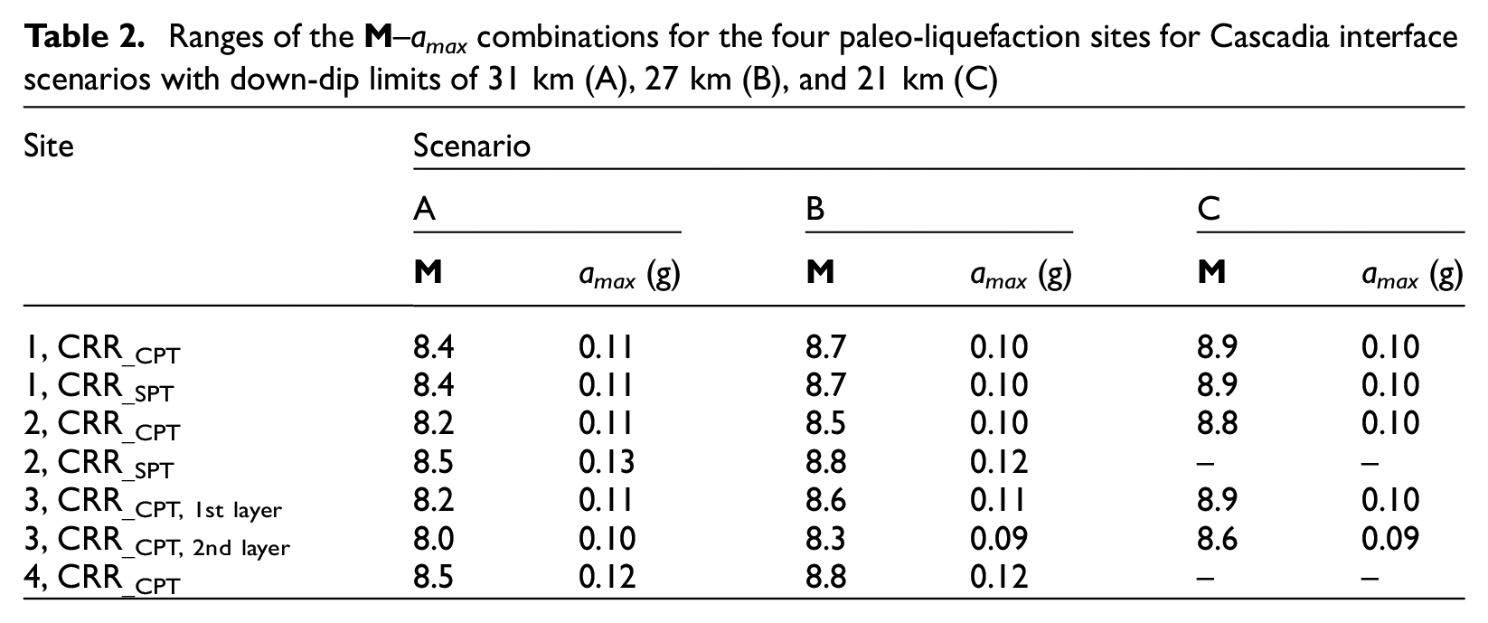
Table 2 lists the back-calculated M–a_max combinations using CPT and SPT inverse analyses and reports the minimum M and a_max expected to initiate liquefaction in the critical layer for each paleo-liquefaction site based on the deterministic framework. For instance, site 1 from scenario B provides minimum M of 8.7 and a_max of 0.10g. The back-calculated analyses express that the minimum required M for triggering liquefaction in the Fraser River delta ranges between 8.0 and 8.9 if we link the liquefaction features to the Cascadia subduction zone. This range of M depends on the site characterization and the selected down-dip limit to determine the distance from the Cascadia fault. The back-analysis technique also provided the minimum a_max range of 0.09–0.13g to have caused liquefaction at the proposed sites within the last 3500 years. Scenario B, the second shortest site-to-source distance, presents M of 8.3–8.8. Scenario C, with the shallowest down-dip limit, and the farthest fault distance to the site, indicates a minimum M of 8.6–8.9. No intersection was found between the boundary lines for scenario C at site 4 as MSF ≤ 9.

Table 2.

Ranges of the M–a_max combinations for the four paleo-liquefaction sites for Cascadia interface scenarios with down-dip limits of 31 km (A), 27 km (B), and 21 km (C)

Site	Scenario
	A		B		C
	M	amax (g)	M	amax (g)	M	amax (g)
1, CRR_CPT	8.4	0.11	8.7	0.10	8.9	0.10
1, CRR_SPT	8.4	0.11	8.7	0.10	8.9	0.10
2, CRR_CPT	8.2	0.11	8.5	0.10	8.8	0.10
2, CRR_SPT	8.5	0.13	8.8	0.12	–	–
3, CRR_CPT, 1st layer	8.2	0.11	8.6	0.11	8.9	0.10
3, CRR_CPT, 2nd layer	8.0	0.10	8.3	0.09	8.6	0.09
4, CRR_CPT	8.5	0.12	8.8	0.12	–	–

Probabilistic assessment of paleo-liquefaction sites

The simplified procedure to determine CSR and CRR is a deterministic approach in which representative or average values are often used. The deterministic framework has inconsistency since the 16^th percentile CRR curve is used with the 50^th percentile a_max (Green et al., 2005). Such inconsistency is also present in the forward analyses of liquefaction as the deaggregation results from the probabilistic seismic hazard analysis (PSHA) for a_max at the return period of interest and mean or modal M are used (Franke et al., 2016). In this way, the ground motions are determined probabilistically, and the liquefaction evaluation is performed deterministically. Therefore, we performed an alternative probabilistic method for paleo-liquefaction analysis. Any one of the combinations of boundary and GMPE curves shown in Figure 5 would be communicated as a deterministic solution. In a probabilistic approach, every combination of CRR and CSR is associated with a probability of liquefaction. Several empirical CPT and/or SPT-based relationships for probabilistic liquefaction triggering have been proposed by Juang et al. (2002), Cetin et al. (2004), Moss et al. (2006), and Boulanger and Idriss (2012, 2014). These different simplified methodologies for evaluating liquefaction assessment were developed based on various assumptions and correlations to obtain parameters such as stress reduction factor, overburden correction factor, and magnitude scaling factor (Guan and Wang, 2022). Thus, we can conclude that these probabilistic methods for CRR and CSR calculations may have significant uncertainty in the simplified methodology or liquefaction model. The liquefaction model uncertainty, σ_lnR, is the standard deviation associated with only epistemic uncertainty of CRR in liquefaction assessment (Franke and Olson, 2021). This model uncertainty only affects the position of the CRR boundary curve. Guan and Wang (2022) considered model uncertainty in the probabilistic analyses of liquefaction via the Monte Carlo simulation. There are also aleatory uncertainties in two principal inputs, CRR and CSR, which are introduced as parameter uncertainties. In this section, we first evaluate the paleo-liquefaction sites considering only model uncertainty and then incorporate both model and parameter variabilities.

We use the probabilistic CPT- and SPT-based methodologies proposed by Boulanger and Idriss (2012, 2014) in a backward analysis for our paleo-liquefaction sites to include the liquefaction model uncertainty. The conditional probability of liquefaction for known parameters of q_c1Ncs and CSR_{M=7.5, σ’ = 1atm} is calculated by the CPT-based liquefaction triggering relation of Boulanger and Idriss (2014):

$$\begin{array}{c}{P}_L(q_{c1\mathrm{Ncs}},\mathrm{CS}{R}_{M=7.5,{\sigma }_v^{\prime }=1\mathrm{atm}})\hfill \\ =\phi \{-\frac{\frac{q_{1\mathrm{cNcs}}}{113}+{\left(\frac{q_{1\mathrm{cNcs}}}{1000}\right)}^2-{\left(\frac{q_{1\mathrm{cNcs}}}{140}\right)}^3+{\left(\frac{q_{1\mathrm{cNcs}}}{137}\right)}^4-2.60-\ln (\mathrm{CS}{R}_{M=7.5,{\sigma }_v^{\prime }=1\mathrm{atm}})}{{\sigma }_{\ln (R)}}\}\hfill \end{array}$$

(2)

$$\mathrm{CS}{R}_{M=7.5,{\sigma }_v^{\prime }=1\mathrm{atm}}=0.65\frac{{\sigma }_v}{{\sigma }_v^{\prime }}\frac{a_{\max }}{g}{r}_d\frac{1}{\mathrm{MSF}}\frac{1}{K_{\sigma }}$$

(3)

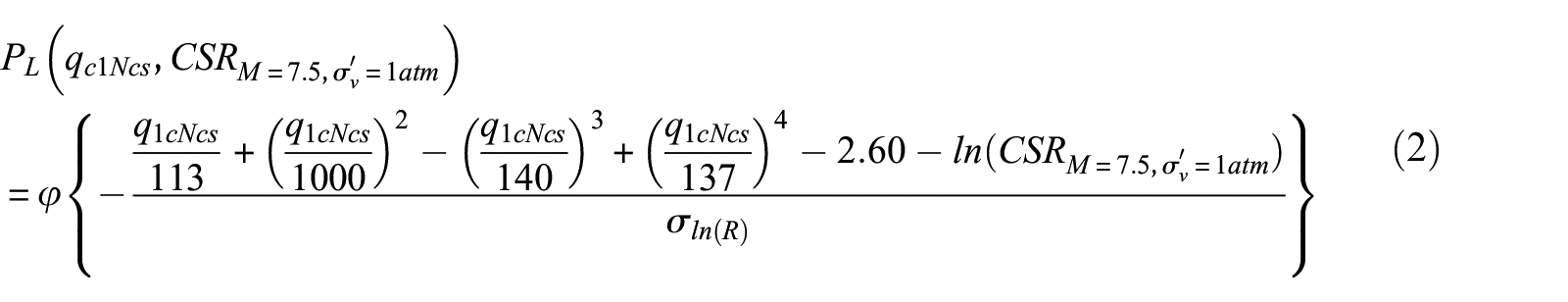
where $\phi$   is the standard normal cumulative distribution function, q_c1Ncs is the equivalent clean sand penetration resistance corrected for overburden pressure and FC, and σ_lnR is the CPT-based liquefaction model uncertainty (ignoring the parameter variability) suggested as 0.2 by Boulanger and Idriss (2014).

For the SPT profiles adjacent to sites 1 and 2, we use the probabilistic SPT-based liquefaction relationship developed by Boulanger and Idriss (2012):

$$\begin{array}{c}{P}_L({(N_1)}_{60\mathrm{cs}},\mathrm{CS}{R}_{M=7.5,{\sigma }_v^{\prime }=1\mathrm{atm}})\hfill \\ =\phi \{-\frac{\frac{{(N_1)}_{60\mathrm{cs}}}{14.1}+{\left(\frac{{(N_1)}_{60\mathrm{cs}}}{126}\right)}^2-{\left(\frac{{(N_1)}_{60\mathrm{cs}}}{23.6}\right)}^3+{\left(\frac{{(N_1)}_{60\mathrm{cs}}}{25.4}\right)}^4-2.67-\ln (\mathrm{CS}{R}_{M=7.5,{\sigma }_v^{\prime }=1\mathrm{atm}})}{{\sigma }_{\ln (R)}}\}\hfill \end{array}$$

(4)

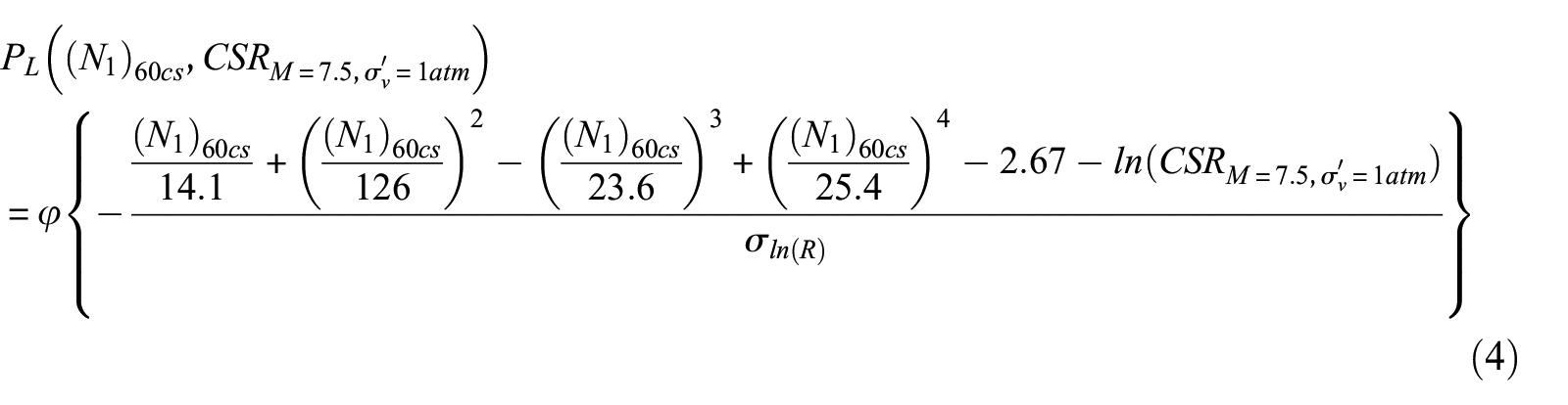
where (N₁)_60cs is the clean sand equivalent SPT resistance corrected for energy ratio, overburden pressure, and FC, and σ_lnR = 0.13 suggested by Boulanger and Idriss (2012). Note that the 16% probability of liquefaction is equivalent to the deterministic triggering correlation for both CPT- and SPT-based methods.

We solve Equations 2 and 4 using the CPT and SPT data at our four sites inclusive of the suggested σ_lnR values and display the triggering curves for probabilities of 16% and 50% of liquefaction in Figure 5. In the same way as in the previous section, the GMPEs are applied deterministically to determine the credible combination of M–a_max. In other words, the median a_max value from the equally weighted four GMPEs is considered without any variability. Instead of the FS = 1 boundary line from the deterministic approach, we now use different probabilities of liquefaction (P_L) for sites 1–4 to estimate the minimum M and a_max from Figure 5. The lower bound of the deterministic approach aligns with the P_L = 16% curve as expected. These curves provide the reader with the acceptable combination of M–a_max for the liquefaction probability of interest. The selection of P_L could be connected to the severity of liquefaction features, for example, number of sand blows, their thickness, and width of sand dykes (Rodriguez-Marek and Ciani, 2008). For example, the existence of sand blows and larger 25–35 cm wide sand dykes at paleo-liquefaction sites 1–3 may better relate to a P_L closer to 50% compared to the smaller sand dykes and no observation of sand blows at site 4 that may better relate to a P_L close to 16% (equivalent to FS = 1).

There are also liquefaction manifestation models (LPIs) to predict sand blows and lateral spreads from liquefaction phenomena. One of the most common of these models is the liquefaction potential index (LPI) proposed by Iwasaki et al. (1982) which determines the liquefaction potential along a soil profile from the ground surface to a depth of 20 m. From empirical seismic-induced liquefaction inventories, LPI > 5 were correlated with the occurrence of sand boils and LPI > 12 were correlated with lateral spreading occurrences. LPI > 5 is generally accepted as a threshold value for surface damage of liquefaction by Iwasaki et al. (1982), Toprak and Holzer (2003), and Holzer et al. (2006). The use of LPI would allow us to interpret the P_L curves for sand blow prediction. For instance, we considered P_L = 50% and obtained the combination of M–a_max for each site. In this way, site 2 has the lowest M and a_max compared to other sites (M = 8.5, a_max = 0.12 g). If we accept this M–a_max combination for the earthquake scenario that caused liquefaction in the region, then we can calculate the associated LPI for each site. For sites 1–3, we calculated LPIs between 5 and 12 which correspond to sand blow manifestations of liquefaction consistent with sand blow observations at these paleo-liquefaction sites. The same M–a_max combination results in an LPI < 5 for site 4 which corresponds to no manifestations of liquefaction and is consistent with the paleo-liquefaction observation of a sand dyke at 2 m depth (liquefaction did not reach surface).

As the changes in soil properties following liquefaction are often unknown, questions remain regarding the application of post-liquefaction geotechnical field investigations for paleo-liquefaction assessment. We selected the representative q_c1Ncs for each paleo-liquefaction site in the previous sections. However, this selection is based on engineering judgment and adds uncertainty to our analyses. While aging and secondary compression could also affect cone tip resistance (Gheibi and Gassman, 2016), these were beyond the scope of our study. Using the current in situ measurements in a paleo-liquefaction assessment may overestimate M–a_max because of the increased density and penetration resistance of the in situ sand following the paleo-liquefaction event(s). Sands generally densify by cyclic loading, so the pre-earthquake penetration resistances (CPT or SPT) would have been lower than the current in situ data. As a result, we would be overestimating CRR, and therefore the liquefying M–a_max combination. We adopted Obermeier et al.’s (2005) recommendations to estimate the historic GWT. This is a qualitative approach, and one can come up with different GWTs based on their interpretation of liquefaction features. Uncertainty in input parameters (e.g. soil properties and ground motion characteristics) is a major limitation of deterministic liquefaction analysis methods. We advance inclusion of CRR and CSR uncertainties into probabilistic back-calculation analyses. Note that we do not try to incorporate the uncertainties of all parameters into the probabilistic methodology. Our proposed framework is shown in Figure 6. For brevity, we only use the simplified CPT-based liquefaction triggering methodology. The probabilistic procedure can be used equally for SPT-based liquefaction analysis. As mentioned before, the probabilistic framework for paleo-liquefaction assessment was developed by Rodriguez-Marek and Ciani (2008) and Maurer et al. (2015). While Maurer et al. (2015) used the probabilistic liquefaction evaluation method proposed by Cetin et al. (2004) for SPT data, we incorporate the probabilistic relationship for CPT profiles by Boulanger and Idriss (2014), that is, Equation 2, and include additional parameter uncertainties to our analyses. Since the probabilistic CPT-based relationship of Boulanger and Idriss (2014) is based on only the model uncertainty, we need to expand Boulanger and Idriss (2014) formulations of CRR and CSR to include parameter uncertainties. Greenfield and Grant (2020) expanded the Boulanger and Idriss (2012) probabilistic SPT-based method and we follow the same procedure for the CPT-based methodology. Franke and Olson (2021) suggested using a logic tree approach or a Monte Carlo simulation to incorporate parameter uncertainties. In this article, we employed Monte Carlo simulations to represent uncertainties in soil resistance, groundwater elevation, maximum acceleration, and the simplified method in a paleo-liquefaction assessment (Figure 6). A probabilistic framework allows for the range of possible causative earthquake magnitudes to be better quantified. We note that the probabilistic methodology is not restricted to backward analyses and could be also applied in a forward evaluation of liquefaction. The proposed methodology is also applicable to other liquefaction sites globally.

Figure 6.

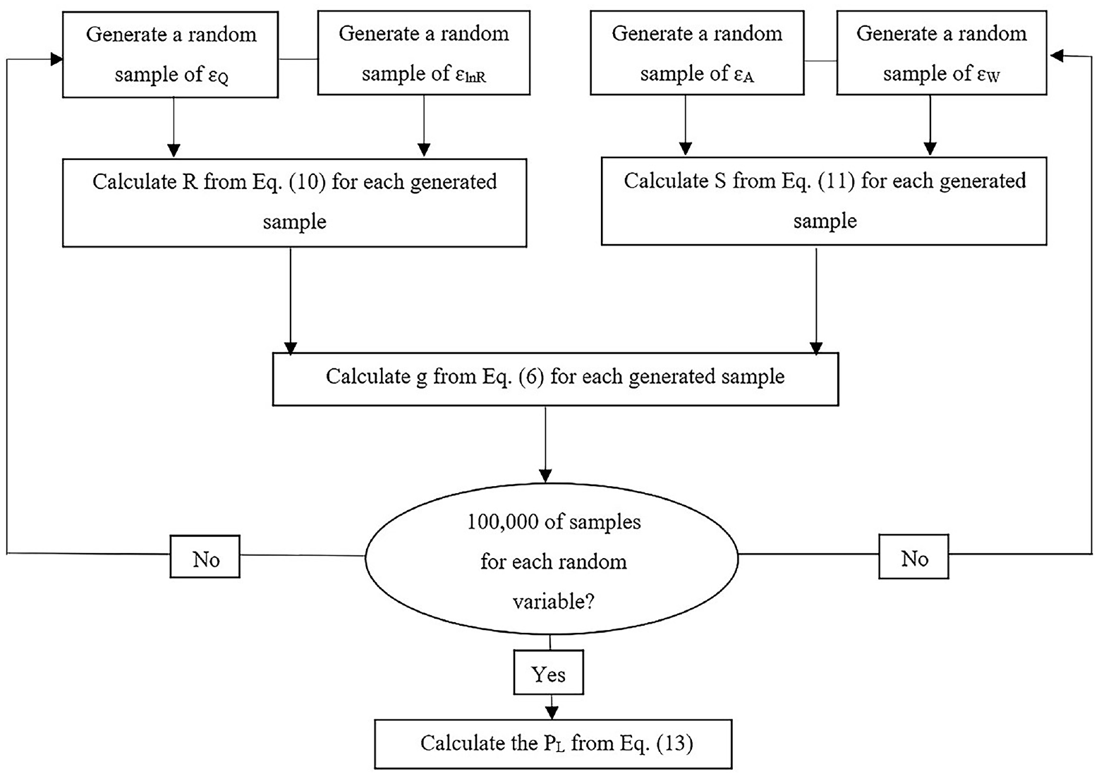
Flowchart of the proposed probabilistic liquefaction analysis framework.

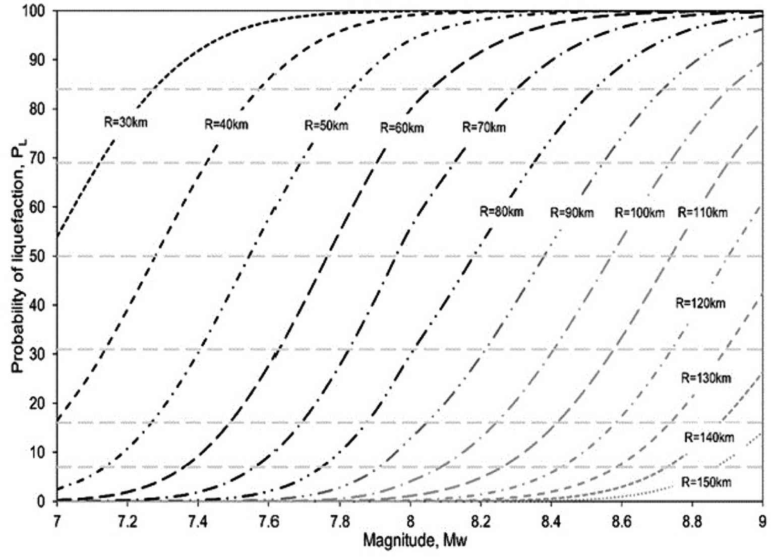
The purpose of the Monte Carlo simulation is to generate random samples to simulate appropriately distributed values of the variables of concern and to repeat a large number of trials to evaluate the statistical characteristics of the dependent variable. This procedure incorporates parameter uncertainty into the probabilistic assessment of paleo-liquefaction sites. We consider q_c1Ncs, z_w (depth of GWT), and a_max as random variables to incorporate their variabilities into the probabilistic framework in Figure 6. We define the mean and variance of each random variable before conducting Monte Carlo random sampling. With the assumption of a normal distribution for q_c1Ncs, we calculated the mean and the standard deviation of cone resistance considering all q_c1Ncs values over the entire critical layer for each paleo-liquefaction site. We also assume a normal distribution for z_w (Haldar and Tang, 1979). The coefficient of variation (CV) of z_w was obtained from the present interpolated GWT map of the Fraser River delta (0.3). The uncertainty in the prediction of a_max is represented by a lognormal distribution with average and standard deviation determined from equal weighting of a_max from the four interface GMPEs (Abrahamson et al., 2008). Using the total probability theorem to integrate over the selected uncertainties, we determine the probability of liquefaction conditional to magnitude and closest fault distance of a Cascadia interface earthquake as:

$$P(\mathrm{Site}\mathrm{liquefies}|M_w,R_{\mathrm{cd}})=\underset{a_{\max }}{\int }\underset{q_{c1\mathrm{Ncs}}}{\int }\underset{z_w}{\int }\begin{array}{c}P(\mathrm{site}\mathrm{liquefies}|a_{\max },q_{c1\mathrm{Ncs}},z_w)f(a_{\max }|M_w,R_{\mathrm{cd}})f\left(q_{c1\mathrm{Ncs}}\right)f\left(z_w\right)\hfill \\ \multicolumn{1}{c}{d{z}_{w}d{q}_{c1\mathrm{Ncs}}d{a}_{\max }}\end{array}$$

(5)

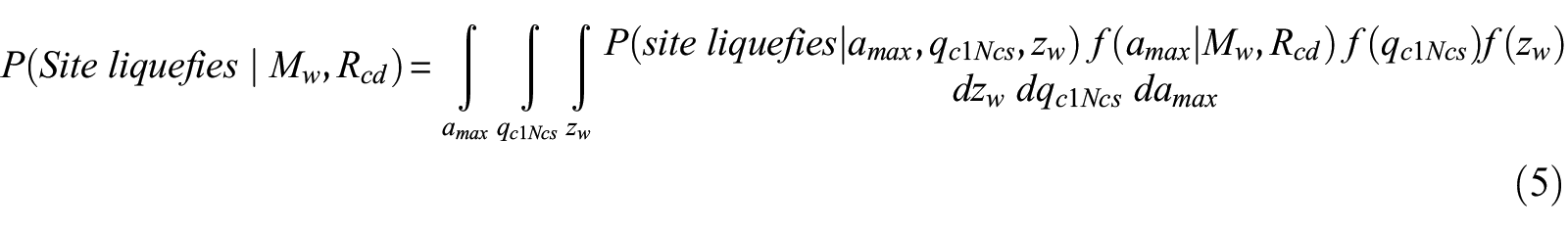
The above integral is similar to the hazard integral used in PSHA and allows us to directly account for the likelihood of liquefaction associated with each paleo-liquefaction site. The term P(site liquefies| a_max, q_c1Ncs, z_w) is the conditional probability of liquefaction by Boulanger and Idriss (2014) for the range of seismic demand from GMPE variability, soil characterization (i.e. uncertainty in selected q_c1Ncs values), and the groundwater depth. The f(a_max| M, R_cd) is the conditional probability density function of a_max. The probability density functions of q_c1Ncs and z_w are represented by f(q_c1Ncs) and f(z_w), respectively. Note that variations in groundwater depths add uncertainty to the calculation of effective vertical stress. One method to solve this integral is using the Monte Carlo simulation. It is a useful tool for estimating probability when the analytical results are difficult to obtain. We repeatedly generated random samples from the prescribed probability distributions of the selected variables and then input these uncertainties into a liquefaction model to calculate the corresponding probability of liquefaction.

We demonstrate here how parameter uncertainties are incorporated into Equation 2’s probabilistic CPT-based relation. Boulanger and Idriss (2014) reformulated the simplified liquefaction procedure using a limit state function, g, with the inclusion of parameter uncertainties:

$$g=\mathrm{lnR}-\mathrm{lnS}$$

(6)

$$R=\mathrm{CR}{R}_{M=7.5,{\sigma }_v^{\prime }=1\mathrm{atm}}$$

(7)

$$S=\mathrm{CS}{R}_{M=7.5,{\sigma }_v^{\prime }=1\mathrm{atm}}$$

(8)

$$g=\hat{\mathrm{g}}+{\epsilon }_T$$

(9)

where R is a random variable for CRR, S is a random variable for CSR, ĝ shows the imperfection of the g function to predict liquefaction, and ε_T is a total error term to consider both the inability of ĝ to predict liquefaction perfectly and the uncertainty in the parameters (Boulanger and Idriss, 2014). Liquefaction occurs when g ≤ 0. We calculate R from the below formula adding model and q_c1Ncs uncertainties:

$$\mathrm{lnR}=\frac{{(q_{c1\mathrm{Ncs}})}_{\mathrm{av}}+{\epsilon }_Q}{113}+{\left(\frac{{(q_{c1\mathrm{Ncs}})}_{\mathrm{av}}+{\epsilon }_Q}{1000}\right)}^2-{\left(\frac{{(q_{c1\mathrm{Ncs}})}_{\mathrm{av}}+{\epsilon }_Q}{140}\right)}^3+{\left(\frac{{(q_{c1\mathrm{Ncs}})}_{\mathrm{av}}+{\epsilon }_Q}{137}\right)}^4-2.6+{\epsilon }_{\mathrm{lnR}}$$

(10)

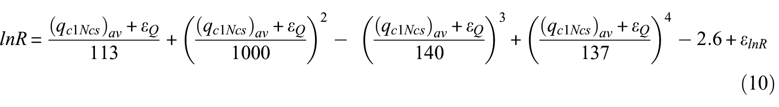
where ε_Q is a normally distributed random variable (Figure 6) to account for the parameter uncertainty in q_c1Ncs with zero mean and variance (σ_Q)², ε_lnR is a random variable (see Figure 6) to consider model uncertainty in CRR with zero mean and variance (σ_lnR)², and (q_c1Ncs) _av is the average value of q_c1Ncs over the critical layer. We also embed the uncertainties of a_max and z_w in the CSR calculation as follows:

$$\mathrm{lnS}=\ln \left(\frac{0.65r_d}{\mathrm{MSF}{k}_{\sigma }}\right)+\ln ({(a_{\max })}_{\mathrm{av}}+{\epsilon }_A)+\ln \left(\frac{{\sigma }_v}{{\sigma }_v-{\gamma }_w.\{z-[{(z_w)}_{\mathrm{av}}+{\epsilon }_W]\}}\right)+{\epsilon }_{\mathrm{lnS}}$$

(11)

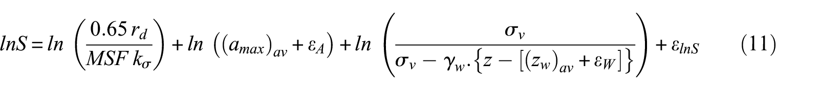
where ε_A is a normally distributed random variable (Figure 6) to account for the uncertainty in a_max with zero mean and variance (σ_A)², ε_W is a normally distributed random variable (Figure 6) to account for the uncertainty in z_w with zero mean and variance of (σ_W)², ε_lnS is a random variable to account for uncertainty in CSR. (a_max) _av and (z_w) _av are the average values. By substituting R and S from Equations 10 and 11 into Equation 6, the mean value of the limit state function is obtained. The variance of the limit state function is calculated using first-order second-moment approximation as:

$$\begin{array}{c}\multicolumn{1}{c}{({\sigma }_T{)}^2=(\frac{1}{113}+\frac{2q_{c1\mathrm{Ncs}}}{{1000}^2}-\frac{3{(q_{c1\mathrm{Ncs}})}^2}{{140}^3}+{\frac{4{(q_{c1\mathrm{Ncs}})}^3}{{137}^4})}^2({\sigma }_Q{)}^2+{\left(\frac{{\gamma }_w}{{\sigma }_v-{\gamma }_w(z-z_w)}\right)}^2({\sigma }_w{)}^2+({\sigma }_A{)}^2}\\ +({\sigma }_{\mathrm{lnR}}{)}^2+({\sigma }_{\mathrm{lnS}}{)}^2\hfill \end{array}$$

(12)

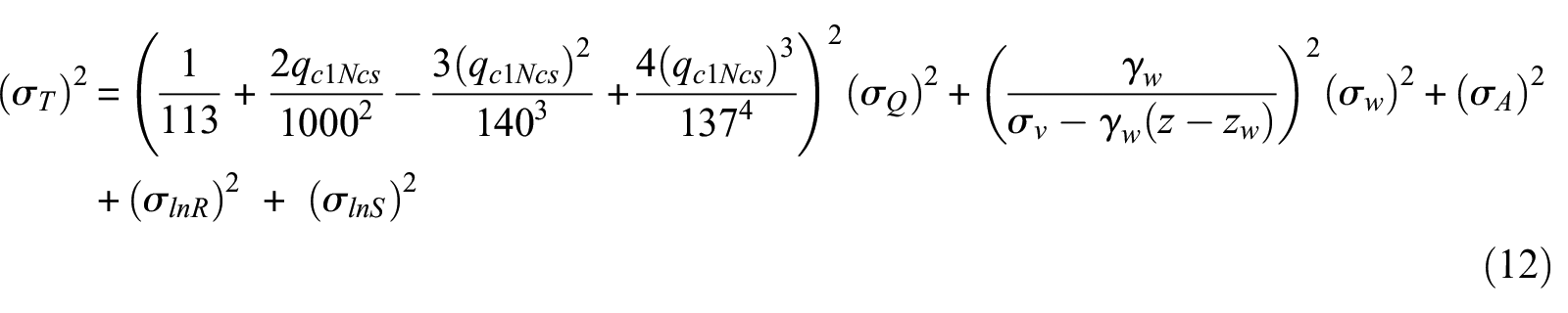
where σ_T is the total uncertainty or the standard deviation of the limit state function.

Using ε_Q and the mean value of q_c1Ncs, we generated 100,000 random values of q_c1Ncs from $(q_{c1\mathrm{Ncs}}{)}_{\mathrm{av}}+{\epsilon }_Q$ for each paleo-liquefaction site according to their normal probability density function as shown in Figure 12 in Appendix 1. We randomly generated error terms of ε_Q, ε_lnR, ε_A, and ε_W (100,000 samples) and applied them in R and S formulas and obtained FS = exp(g) for each analysis iteration. We calculate the probability of liquefaction by dividing the number of times that the limit function satisfies the g ≤ 0 condition by the total number of simulations as:

$$P_L=\frac{N_{\mathrm{liq}}}{N}$$

(13)

where N is the total number of simulations, and N_liq is the number of samples where liquefaction occurs (g ≤ 0).

The flowchart of Figure 6 was repeated for an M range of 7–9 with an increment of 0.1 with each M associated with each of the three plausible down-dip depth limits to calculate the corresponding probability of liquefaction for the four paleo-liquefaction sites. Note that we did not include the uncertainties of other parameters such as total stress or stress reduction factor in our probabilistic methodology. However, we believe that incorporating other parameters’ uncertainties is feasible by following similar steps. The accuracy of the calculated P_L depends on the number of generated random samples. A preliminary convergence analysis proved that the P_L values were almost identical when the number of simulations changed from 100,000 to 1,000,000. Therefore, to reduce the run time of analyses, we selected 100,000 as the optimum number for generating stochastic variables.

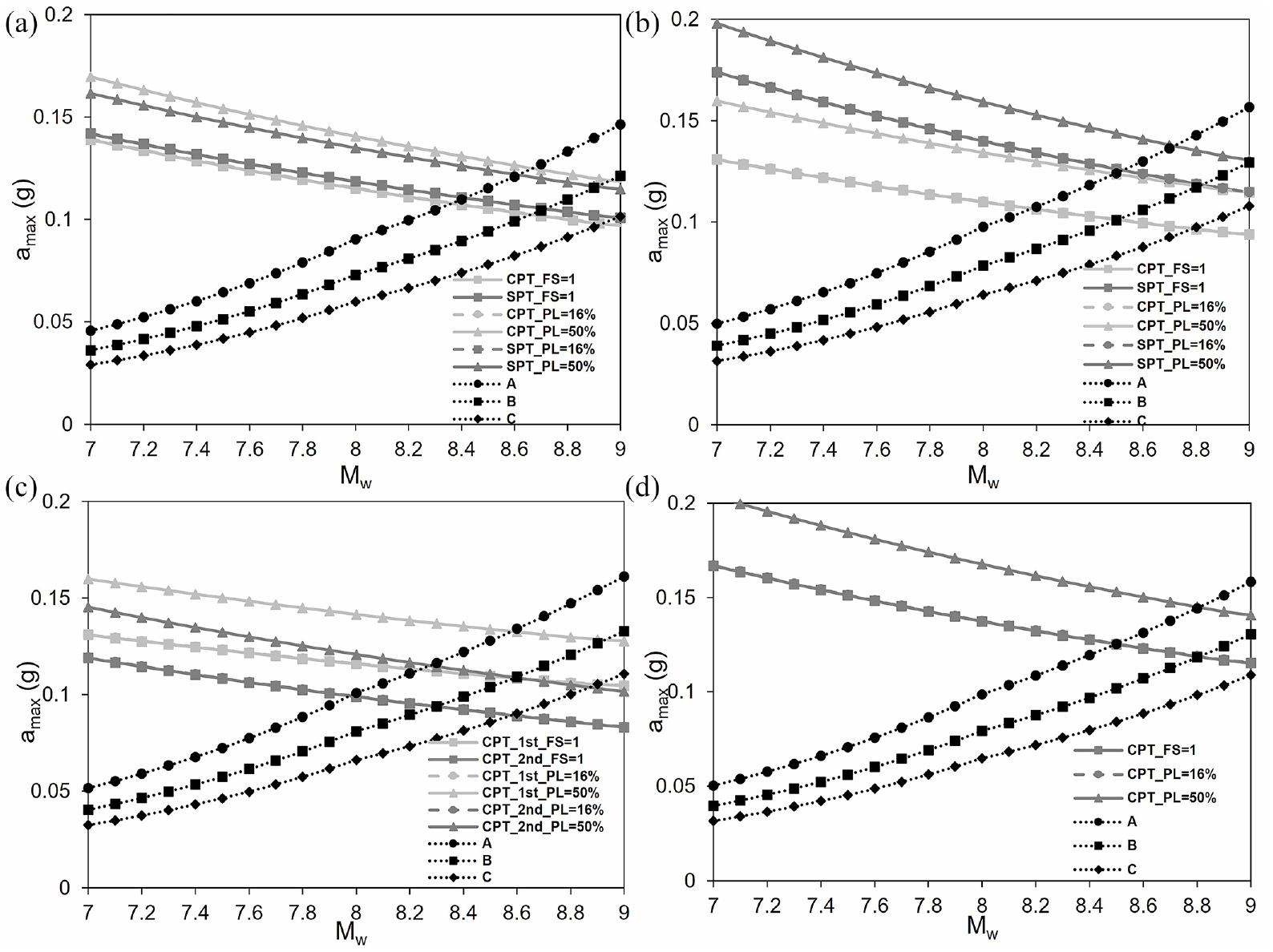
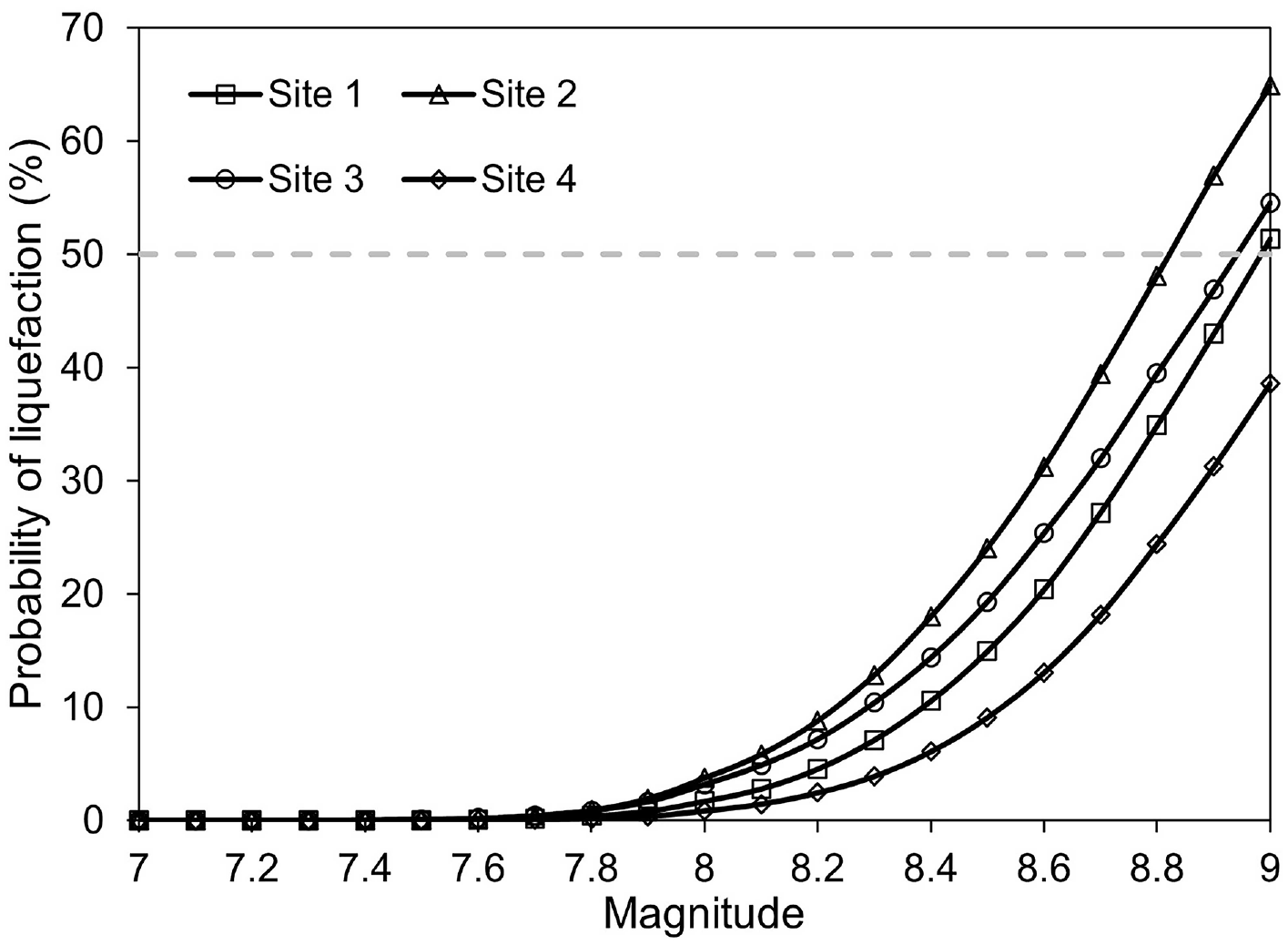
Figure 7 displays the probability of liquefaction for a range of M given the three plausible down-dip limits for each paleo-liquefaction site. For site 3, we used the first critical layer in the probabilistic analysis. These liquefaction probability plots incorporate uncertainties in the prediction of a_max and the liquefaction model, as well as the selection of q_c1Ncs and z_w values. In addition, Figure 7 reflects the down-dip limit uncertainty in the site-to-source distance. Note that P_L = 16% would not produce similar results with the deterministic analysis because of adding parameter uncertainty. From Figure 7, we can estimate the probable M for a range of liquefaction probabilities. Table 3 reports the M range when the probability of liquefaction is 16% (i.e. deterministic or FS = 1) and 50% (median or best estimate) for each paleo-liquefaction site. For instance, M = 8.6–9.0 are estimated at site 1 given a down-dip limit of scenario B.

Figure 7.

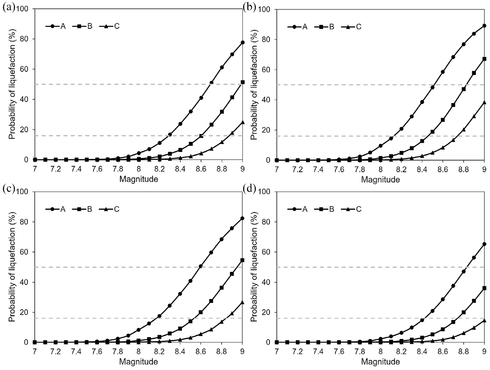
Probability of liquefaction versus interface earthquake magnitude considering three down-dip limits (A–C) for (a) site 1, (b) site 2, (c) site 3, and (d) site 4. Dashed lines denote P_L = 16% and 50%.

Table 3.

Ranges of M for liquefaction probabilities of 16%–50%

Site	Magnitude range
	Scenario A	Scenario B	Scenario C
1	8.3–8.7	8.6–9.0	8.9–9.0*
2	8.1–8.5	8.5–8.8	8.8–9.0*
3	8.2–8.6	8.5–9.0	8.9–9.0*
4	8.4–8.8	8.8–9.0*	9.0*

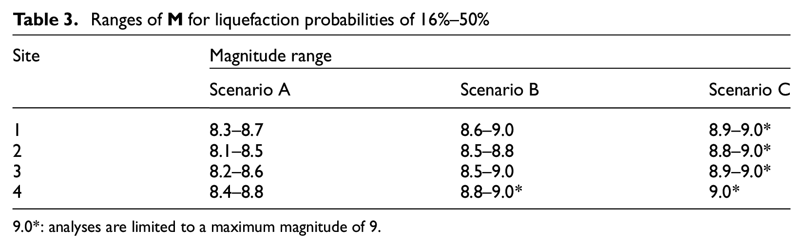
9.0*: analyses are limited to a maximum magnitude of 9.

One of the limitations of the deterministic framework is the selection of the correct down-dip limit of M 7–9 Cascadia interface earthquake ruptures. The NBCC 2020 defines three equally weighted down-dip limits for the Cascadia interface fault source. Therefore, we use equal weighting of the three down-dip limits to include the source rupture uncertainty to the paleo-liquefaction assessment. Figure 8 shows the probability of liquefaction versus magnitude for all paleo-liquefaction sites, including the source rupture variability. In our study area, the probability of liquefaction of a Cascadia mega-thrust interface earthquake spans from 1%–4% for M < 8 to 31%–57% for M > 8.9. The P_L curves show that the probability of liquefaction for each site and its variance among the four sites increases with earthquake magnitude. At M 9, site 2 shows a 69% probability of liquefaction, while site 4 has a 39% probability of liquefaction. The increasing variation of P_L curves for different sites with increasing magnitude is likely controlled by their different soil capacity resistance. The M corresponding to P_L = 16% ranges from 8.4 to 8.7. The best-estimate M is related to a 50% probability of liquefaction (Maurer et al., 2015). The M corresponding to P_L = 50% for sites 1, 2, and 3 are 9.0, 8.8, and 8.9, respectively. For site 4, the highest probability of liquefaction is 39% and the best estimate of M is higher than 9.0. Note that we have limited our analyses to M = 9.0, which is the largest M in the MSF formula.

Figure 8.

Probability of liquefaction versus interface earthquake magnitude including uncertainty in the source rupture area.

Developing magnitude-bound curves specific to Cascadia interface earthquakes

The magnitude-bound curves of Ambraseys (1988) and Papadopoulos and Lefkopoulos (1993) are developed based on global liquefaction field observations. It is also possible to generate these curves by back-calculating M and a_max values from regional GMPEs. We assume one representative soil resistance profile to construct magnitude-bound curves for Cascadia interface earthquakes specific to the Fraser River delta. The selected representative q_c1Ncs value is 103 determined as the average of four paleo-liquefaction sites studied in the previous sections. We consider z_w = 1 m and V_s30 = 180 m/s and use a bin size increment of 10 km for distance and 0.1 for magnitude. This corresponds to representative ASCE 7-22 seismic site class E designation. The deterministic lower bound curve was generated using the Boulanger and Idriss (2014) simplified method. We also account for the minimum peak acceleration, (a_max) _t , required to induce a threshold shear strain (10⁻⁴) below which cyclic pore water pressure would not be generated and thereby liquefaction would not occur regardless of the shaking duration (Dobry et al., 1982). This limiting (a_max) _t affects the shape of the magnitude-bound curve for far-field earthquakes (Maurer et al., 2015). All a_max values back-calculated from our deterministic analysis are higher than (a_max) _t , and thus, the magnitude-bound curves would not be affected by a threshold shear strain. The intersection of the representative site’s boundary curve (FS = 1) with the weighted average of the four interface GMPEs (Figure 13 in Appendix 1) provides the minimum M required to produce liquefaction at fault-to-site distances of 50–150 km, from which the back-calculated magnitude-bound relation corresponding to the deterministic analysis can be obtained.

In the probabilistic framework of generating magnitude-bound curves, we only added model uncertainty and the variability of GMPEs for simplicity and to reduce the analysis run time. Therefore, Equation 5 reduced to:

$$P(\mathrm{Site}\mathrm{liquefies}|M_w,R_{\mathrm{cd}})=\underset{\mathrm{amax}}{\int }P(\mathrm{site}\mathrm{liquefies}|a_{\max })f(a_{\max }|M_w,R_{\mathrm{cd}})d{a}_{\max }$$

(14)

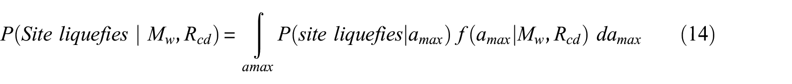
We calculated Equation 14 for individual earthquake magnitudes (7–9) and fault-to-site distances (30–150 km) to generate liquefaction probability curves (Figure 9). From these liquefaction probability curves, probabilistic magnitude-bound curves were back-calculated. We chose P_L = 7%, 16%, 31%, 50%, 69%, and 85% to form the magnitude-bound curves from Figure 9 with the probabilistic framework (Equation 14). Since the closest distance of the study area from the Cascadia subduction zone is 100 km, earthquakes with M less than 8.0 have a P_L of almost zero using the R = 100 km curve. Figure 10 shows the probabilistic and deterministic magnitude-bound curves for Cascadia interface earthquakes in comparison to the two empirical magnitude-bound curves shown earlier in Figure 4. These are the first magnitude-bound curves specific to the Cascadia subduction zone from liquefaction features observed in the Fraser River delta. As expected, the P_L = 16% magnitude-bound curve closely aligns with the deterministic one. The P_L = 16% or deterministic curve may significantly underestimate the earthquake magnitude which caused the paleo-liquefaction features. We tested the formulated P_L = 16% and 50% curves for 12 paleo-liquefaction sites documented in the Fraser River delta. The farthest paleo-liquefaction site located in the Serpentine River floodplain is 135 km from the Cascadia subduction fault. The black circles in Figure 10 represent the 12 paleo-liquefaction sites corresponding to P_L = 16%. This magnitude-bound curve estimates M = 8.3–8.5. The P_L = 50% probability curve is the best M estimate for liquefaction triggering. We display the distances of the 12 paleo-liquefaction sites with black squares in Figure 10. The best-estimate magnitude-bound curve for P_L = 50% corresponds to M = 8.6–8.9 from paleo-liquefaction sites.

Figure 9.

Probability of liquefaction versus earthquake magnitude for a range of fault-to-source distances.

Figure 10.

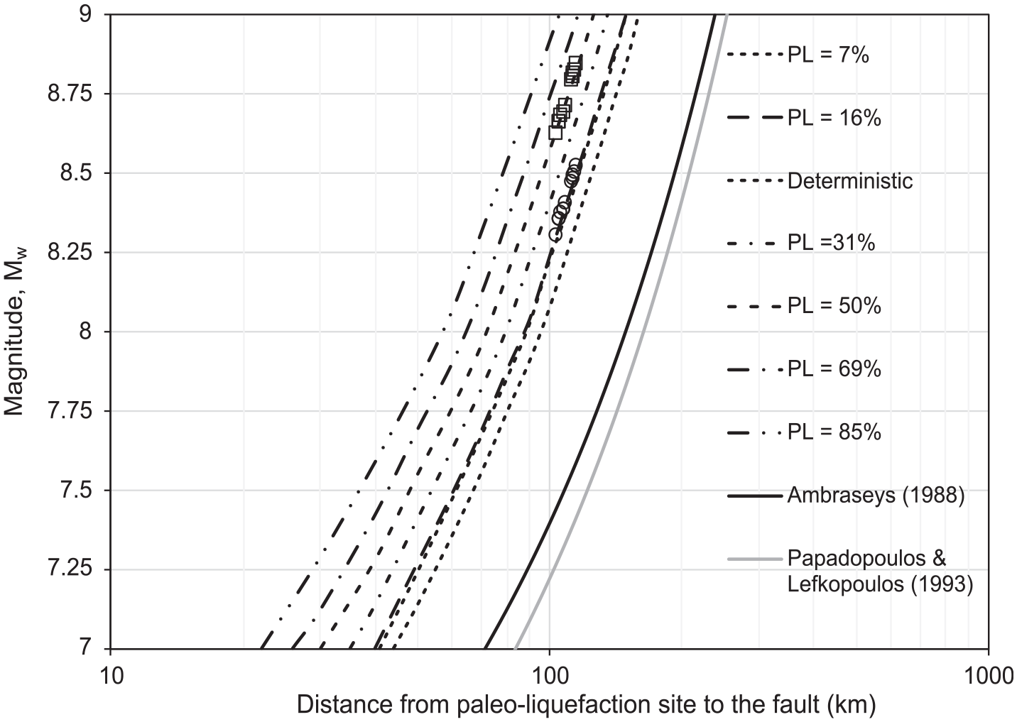
Probabilistic and deterministic back-calculated magnitude-bound relations for the Cascadia subduction zone. Black circles and squares are distances of the 12 paleo-liquefaction sites on the P_L = 16% and P_L = 50% curves, respectively.

The deterministic and probabilistic magnitude-bound relations for the Cascadia subduction zone developed from the Fraser River delta paleo-liquefaction evidence estimates higher paleo-earthquake magnitudes than those obtained from worldwide magnitude-bound curves of Ambraseys (1988) and Papadopoulos and Lefkopoulos (1993). The developed magnitude-bound curve for Cascadia was derived from regional ground motion models and site conditions in the Fraser River delta. Thus, these curves provide a more accurate estimation of magnitude from paleo-liquefaction data for the regions affected by the Cascadia subduction zone. Adding more data from paleo-liquefaction sites nearby the Columbia River (Atwater, 1994) and Humptulips River (Obermeier, 1995) can improve the soil representative site parameter selection and the shape of these curves. It should be mentioned that the absence of liquefaction features in the Fraser River delta from the last great Cascadia interface earthquake in 1700 may be attributed to two explanations. First, the 12 known paleo-liquefaction sites occur primarily in exposed ground and a systematic effort (e.g. trenching) to document paleo-liquefaction throughout the Fraser River lowlands has not been performed. Another possible reason may be that the known paleo-liquefaction features were generated by a nearby crustal earthquake as concluded by the original investigators. The proposed magnitude-bound curves are limited to interface earthquakes from the Cascadia subduction zone using the representative soil resistance with V_s30 of 180 m/s. Readers should consider the limitation of using the generated magnitude-bound curves for other earthquake types. Following the same methodology used in this study, the deterministic and probabilistic magnitude curves could also be generated for the other two earthquake source types (crustal and inslab) in the region if they result in liquefaction triggering.

Conclusion

In this article, we investigated the paleo-liquefaction evidence found in the Fraser River delta region and provided soil characterization of the liquefaction source layers from in situ SPT and CPT measurements. The cyclic stress method was interpreted jointly with updated regional GMPEs for Cascadia interface earthquakes (2020 NBCC) to estimate the minimum moment magnitude and peak ground acceleration required to induce liquefaction features in a deterministic framework. We did not consider a shallow crustal earthquake near Vancouver as the probable seismic source since the location of nearby active crustal faults has greater uncertainty than the known location of the Cascadia subduction zone. The deterministic and probabilistic paleo-liquefaction back-calculation methodologies applied in this article should be used to evaluate the other plausible earthquake source type (nearby active crustal faults) in future.

We started by applying a deterministic approach using three plausible full-rupture scenarios with different down-dip rupture limits (source-to-site distance) to calculate the median a_max for moment magnitudes of 7–9 using the four Cascadia interface GMPEs of the 2020 NBCC. The lower bound on the minimum M from our deterministic back-calculated engineering analysis for four paleo-liquefaction sites ranges from 8.0 to 8.9 and the associated peak ground acceleration ranges from 0.09 to 0.13g if we consider the Cascadia subduction zone as the plausible seismic source. Our findings are consistent with those of Clague et al. (1998) that Cascadia interface earthquakes with M < 8.0 are unlikely to induce liquefaction in the study area. Using an LPI verifies the paleo-liquefaction observations of sand blows at sites 1–3, but not at site 4.

The applied deterministic scenarios could underestimate the associated earthquake magnitude at the paleo-liquefaction sites. In addition, the deterministic framework has inconsistency of using median a_max and the 16^th percentile of liquefaction model. Therefore, we proceeded to applying a probabilistic approach to paleo-liquefaction back-calculation analysis. We note that the probabilistic framework can be applied in either forward liquefaction or back-calculation paleo-liquefaction analyses. The probabilistic assessment of liquefaction features to obtain the best-estimate magnitude allows for the systematic incorporation of uncertainties into the paleo-liquefaction assessment. We incorporate uncertainties of soil resistance, GWT, and peak ground surface acceleration as well as the simplified liquefaction triggering model in our probabilistic paleo-liquefaction assessment using the Monte Carlo method. The methodology not only incorporates parameter uncertainties but also allows the consideration of source-to-site distance variability. Other parameters associated with liquefaction analysis such as vertical stress and r_d can also be treated as random variables in future probabilistic paleo-liquefaction analyses. The median M of Cascadia interface events to produce liquefaction features in the region estimated from our probabilistic methodology for the four considered paleo-liquefaction sites ranges between 8.8 and 9.0. Moreover, the probability curves indicate that there is a 31%–57% likelihood of liquefaction initiation considering a M > 8.9 Cascadia interface event, noting the lowest probability of liquefaction triggering occurs at site 4 due to its higher soil resistance compared to sites 1–3. One limitation of our probabilistic framework was using the current in situ soil resistance measurements (not correcting to a pre-liquefied state) which leads to an upward biased estimation of M. As there are many uncertainties inherent in back-calculation techniques, we recommend using the probabilistic approach over the deterministic methodology for paleo-liquefaction assessment.

Region-specific magnitude-bound curves improve magnitude estimation compared to global correlations. Therefore, we developed magnitude-bound curves in deterministic and probabilistic frameworks for Cascadia interface earthquakes with V_s30 = 180 m/s (site class E). The constructed magnitude-bound curves in this article are more region- and source-specific than empirical global magnitude-bound relationships. Magnitude-bound curves can also be generated in future using the same presented methodology for other seismic source types (e.g. crustal and inslab earthquakes).

Research Data

sj-xlsx-1-eqs-10.1177_87552930231197376 – Supplemental material for Estimation of historical earthquake-induced liquefaction in Fraser River delta using NBCC 2020 GMPEs in deterministic and probabilistic frameworks

Supplemental material, sj-xlsx-1-eqs-10.1177_87552930231197376 for Estimation of historical earthquake-induced liquefaction in Fraser River delta using NBCC 2020 GMPEs in deterministic and probabilistic frameworks by Alireza Javanbakht, Sheri Molnar, Abouzar Sadrekarimi and Hadi Ghofrani in Earthquake Spectra

This article is distributed under the terms of the Creative Commons Attribution 4.0 License (https://creativecommons.org/licenses/by/4.0/) which permits any use, reproduction and distribution of the work without further permission provided the original work is attributed as specified on the SAGE and Open Access pages (https://us.sagepub.com/en-us/nam/open-access-at-sage).