Basin effects from 3D simulated ground motions in the Greater Los Angeles region for use in seismic hazard analyses

Abstract

We develop basin-depth-scaling models (i.e. “basin terms”) from the long-period ( $T\ge 2\mathrm{s}$ ) simulated ground motions of the Southern California Earthquake Center (SCEC) CyberShake project for use in seismic hazard analyses at sites within the sedimentary basins of southern California. Basin terms use the Next Generation Attenuation (NGA)-West-2 ground-motion models (GMMs) as reference models and use their functional forms with slight modifications. We investigate the use of two approaches to incorporate the time-averaged shear-wave velocity in the upper 30 m ( $V_{S30}$ ) in these calculations and find that the use of site-specific and uniform $V_{S30}$ has minor effects on the resulting basin terms for this data set. By centering the simulated ground motions on the basin terms, we separate the information from the simulations about absolute ground-motion level from information relating to the relative amplifications, such as the differences between shallow- and deep-basin sites. Recent observations from sedimentary basins of southern California indicate that additional amplification effect may persist at relatively shallow basin depths (i.e. the GMM basin terms should have positive values when differential depths, $\delta Z_1$ , are near zero), and we present models for “centered” and “adjusted” basin-depth scaling models that reflect this potential. The simulation-modified GMMs are appropriate for crustal sources and for deep-basin sites ( $\delta Z_1>0$ ) within basins of the Greater Los Angeles region, for the magnitudes and distances defined by each of the reference NGA-West-2 GMMs.

Introduction

For more than 30 years, three-dimensional (3D) ground-motion simulations have been used to explain and model ground shaking from observed and expected earthquakes (e.g. Aagaard et al., 2008; Frankel and Vidale, 1992; Graves et al., 1998; Olsen et al., 1997, 2006). Due to the short catalog of instrumental records and the long recurrence times of most moderate- to large-magnitude earthquakes, empirical databases contain a sparse sampling of the larger magnitudes ( $M_W\gtrsim 7$ ) and closer distances ( $R<20\mathrm{km}$ ) that are most important to seismic hazard (Ancheta et al., 2014). The use of 3D simulations has been especially fruitful for modeling ground motions in regions with deep sedimentary basins because of the effects of complex wave propagation and amplification (e.g. Frankel et al., 2009; Komatitsch, 2004; Maufroy et al., 2015). Because computational requirements increase exponentially with the maximum resolved frequency in 3D simulations, and because of the limited understanding of high-frequency source processes and limited knowledge of fine-scale structure, many simulations have been constrained to lower frequencies ( $f\lesssim 1\mathrm{Hz}$ ) (Graves and Pitarka, 2010; Irikura and Miyake, 2011). However, advances in source modeling and computing architectures have increased the maximum frequency of these simulations (Harris et al., 2009; McCallen et al., 2021; Rodgers et al., 2020; Withers et al., 2019), and with improved characterization of seismic velocity structure and the rupture process, accurate and realistic broadband ground-motion simulations are likely to contribute to future seismic hazard assessments.

Ground-motion simulations for earthquake hazards recognize the effect of the random nature—or as-yet unknown and unmodeled details—of the earthquake rupture process on resulting ground motions (Graves et al., 2008; Ripperger et al., 2008). Regional ground-motion studies have made use of multiple realizations of kinematic and dynamic rupture properties (Aagaard et al., 2010; Moschetti et al., 2017; Roten et al., 2011; Wirth et al., 2018b). Studies have also started to combine ground-motion simulations with recurrence information to produce probabilistic ground-motion exceedance curves and maps (Frankel et al., 2007; Graves et al., 2011; Milner et al., 2021).

Use of ground-motion simulations in seismic hazards applications for engineering design has responded to the progress in simulation methods. For example, the functional forms of the basin-amplification terms for some of the ground-motion models (GMMs) of the Next Generation Attenuation (NGA)-West project (Power et al., 2008) were defined by long-period ground-motion simulations of southern California earthquakes (Day et al., 2008). In the US Pacific Northwest, the engineering and scientific communities have continued discussions regarding the use of 3D simulations for design of tall buildings in the Seattle basin (Chang et al., 2014); recent work recommended the use of basin amplifications from simulations of M9 earthquakes on the Cascadia subduction interface for building design (Frankel et al., 2018; Wirth et al., 2018a). In southern California, the engineering and scientific communities developed maximum considered earthquake response spectra that incorporate the 3D simulations of the Southern California Earthquake Center (SCEC) CyberShake project (Graves et al., 2011; Jordan et al., 2018) by combining response spectra from the empirical GMMs and simulated ground motions in a period-dependent logic tree. The development of a nonergodic framework for GMMs presents an alternative way to incorporate simulated ground motions into probabilistic seismic hazard analysis, which can account for spatial variations in simulated output and the effect of improved ground-motion predictions on uncertainties (Abrahamson et al., 2019; Sung and Abrahamson, 2022).

In this article, we use a large subset of the simulated ground motions from the SCEC CyberShake project to develop basin-depth scaling models for empirical GMMs from NGA-West-2 (Bozorgnia et al., 2014) for use in seismic hazard analyses. The basin-depth scaling models are developed with parameterizations that are consistent with the NGA-West-2 GMMs and can thus be used directly with the GMMs for seismic hazards assessments. We evaluate the sensitivity of the basin terms to choices for the time-averaged shear-wave velocity in the upper 30 m ( $V_{S30}$ ) used to compute ground-motion residuals and methods for constraining the absolute level of ground motion. In addition, we compare simulation-derived models with the empirical models.

Data and functional forms for simulation-derived basin-depth scaling models

Simulation-modified GMMs

We develop basin-depth scaling models from simulated ground motions for use with four of the NGA-West-2 GMMs—Abrahamson et al. (2014; ASK14), Boore et al. (2014; BSSA14), Campbell and Bozorgnia (2014; CB14), and Chiou and Youngs (2014; CY14). The simulation-modified GMMs use the empirically derived predictions of each of the reference GMMs—including the source, path, linear $V_{S30}$ -scaling, and nonlinear site-response terms—but replace the empirical basin terms with basin terms derived from CyberShake ground motions, $f_{b,\mathrm{CS}}^{\mathrm{GMM}}$ . The simulation-derived GMMs are parameterized as:

$${\mu }_{\mathrm{ASK}14\_\mathrm{CS}}(M,R,V_{S30},Z_1,\dots )={\mu }_{\mathrm{ASK}14}(M,R,V_{S30},\delta Z_1=0,\dots )+f_{b,\mathrm{CS}}^{\mathrm{ASK}14}\left(Z_1\right)+c_0^{\mathrm{SIM}}$$

(1)

$${\mu }_{\mathrm{BSSA}14\_\mathrm{CS}}(M,R,V_{S30},Z_1,\dots )={\mu }_{\mathrm{BSSA}14}(M,R,V_{S30},\delta Z_1=0,\dots )+f_{b,\mathrm{CS}}^{\mathrm{BSSA}14}\left(Z_1\right)+c_0^{\mathrm{SIM}}$$

(2)

$${\mu }_{\mathrm{CB}14\_\mathrm{CS}}(M,R,V_{S30},Z_{2.5},\dots )={\mu }_{\mathrm{CB}14}(M,R,V_{S30},Z_{2.5}=1.0,\dots )+f_{b,\mathrm{CS}}^{\mathrm{CB}14}\left(Z_{2.5}\right)+c_0^{\mathrm{SIM}}$$

(3)

$${\mu }_{\mathrm{CY}14\_\mathrm{CS}}(M,R,V_{S30},Z_1,\dots )={\mu }_{\mathrm{CY}14}(M,R,V_{S30},\delta Z_1=0,\dots )+f_{b,\mathrm{CS}}^{\mathrm{CY}14}\left(Z_1\right)+c_0^{\mathrm{SIM}}$$

(4)

where the simulation-derived ground-motion predictions of median ground motion are given by (e.g. for the ASK14 GMM) ${\mu }_{\mathrm{ASK}14\_\mathrm{CS}}$ , the median empirical ground-motion prediction is given by ${\mu }_{\mathrm{ASK}14}$ , $M$ is the moment magnitude, $R$ represents the appropriate distance metrics, $V_{S30}$ is the time-averaged shear-wave velocity in the top 30 m, and $Z_1$ and $Z_{2.5}$ are the depths to the 1.0 and 2.5 km/s shear-wave horizons, respectively. In all cases, the modified GMMs use the reference GMM with no additional basin effects (i.e. $\delta Z_1=0$ for ASK14, BSSA14, and CY14 and $Z_{2.5}=1.0$ km for CB14); we recognize that the linear $V_{S30}$ -scaling model captures average basin effects and we thus refer to the $Z_1$ - and $Z_{2.5}$ -based models as modeling basin effects beyond what is modeled by $V_{S30}$ . The basin-depth scaling models computed from the CyberShake simulations are given by $f_{b,\mathrm{CS}}$ . The $c_0^{\mathrm{SIM}}$ terms, which are zero for the empirical GMMs, allow for additional adjustments to the GMMs within the basins of southern California.

Simulated data set

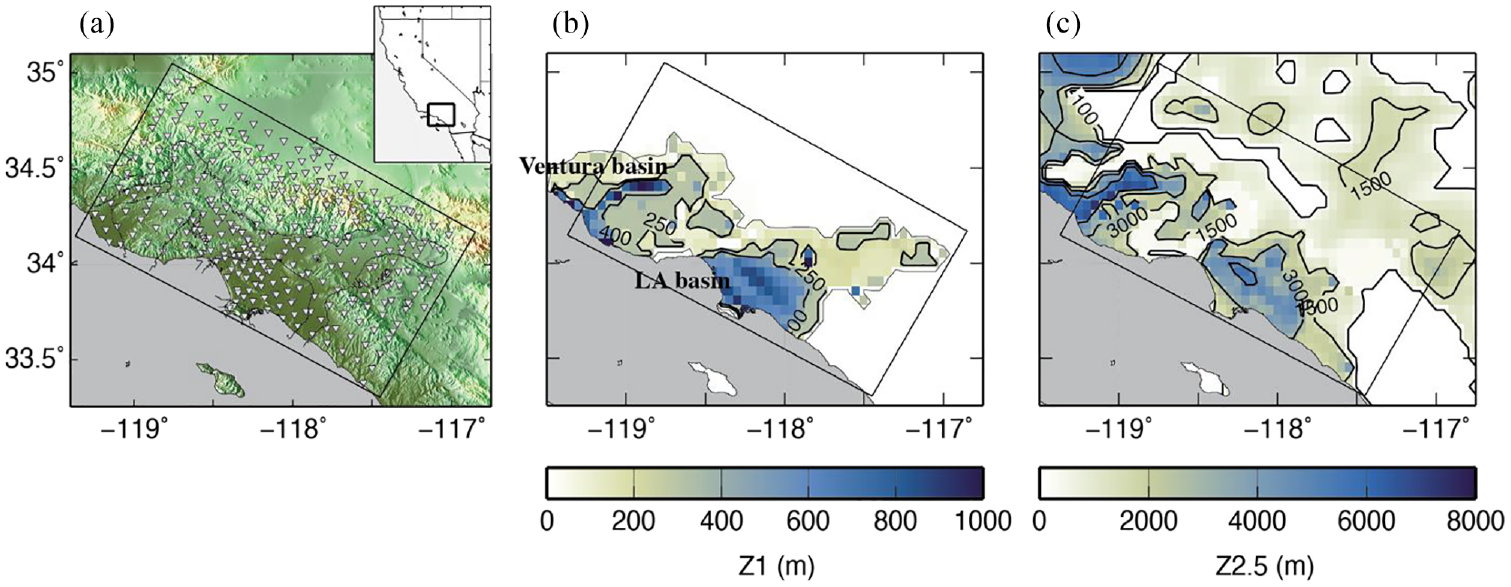
Our analysis uses simulated ground motions from the SCEC CyberShake project 15.4 (Graves et al., 2011; Jordan et al., 2018). CyberShake calculations use the SCEC CVM-S4.26-M01 seismic velocity model, which is a 3D seismic velocity model for southern California based on full-waveform tomography that also includes details of the shallow “geotechnical layer” of the seismic profiles (Lee et al., 2014). Seismic sources are prescribed by the Uniform California Earthquake Rupture Forecast, Version 2 (UCERF2) magnitudes and fault geometries (Field et al., 2009); our calculations do not make use of event rates. For each seismic source, a suite of finite-fault ruptures is created using the Graves and Pitarka (2015) kinematic rupture generator. Each suite of ruptures samples over various hypocenter locations and slip distributions. Because we are interested in the deterministic calculations that capture the long-period basin effects, and these simulations were run with a maximum resolved frequency of 1 Hz, we restrict our analysis to the long-period oscillator values ( $T=2,3,4,5,7.5,10\mathrm{s}$ ). We use 672,000 ground-motion records from 336 sites within the simulation domain (Figure 1) that were selected by random selection of events and stations (Withers et al., 2020). The data set corresponds to about 2% of the full CyberShake data set, which Withers et al. (2020) found sufficient to capture site and basin effects relative to the use of larger data sets.

Figure 1.

Station locations and basin site properties of CyberShake within southern California. (a) Locations of recording stations are depicted with gray triangles within the CyberShake simulation domain and regional context (inset). Depths to the (b) 1 km/s ( $Z_1$ ) and (c) 2.5 km/s ( $Z_{2.5}$ ) shear-wave velocity horizons are plotted from the SCEC CVM-S4.26 seismic velocity model.

Ground-motion residuals

Development of the simulation-derived basin-depth scaling models uses the ground-motion residuals from the four GMMs. We compute ground-motion residuals, $R_{\mathrm{es}}$ , for each of the GMMs:

$$R_{\mathrm{es}}^{\mathrm{GMM}}=\ln \left(S{A}_{\mathrm{es}}\right)-{\mu }_{\mathrm{GMM}}(M,R,V_{S30},\delta Z_1=0,Z_{2.5}=1.0\mathrm{km},\dots )$$

(5)

where $S{A}_{\mathrm{es}}$ are the pseudo-spectral acceleration values from the CyberShake simulations for event e and station s. We refer to the raw residuals of Equation 5 as “uncentered” or unadjusted residuals (i.e. there have not been adjustments to the raw residual values); this term is used in contrast with “centered” residuals, which have been adjusted to match the ground-motion levels of the empirical GMMs at particular basin depths (i.e. $\delta Z_1=0$ or $1\le Z_{2.5}\le 3\mathrm{km}$ ). The GMMs, ${\mu }_{\mathrm{GMM}}$ , are evaluated with site parameters that result in no additional basin effects from the GMMs (i.e. $\delta Z_1=0$ and $Z_{2.5}=1.0\mathrm{km}$ ) and use the shallow site parameter $V_{S30}$ . The $V_{S30}$ parameter is the most widely used parameter for prediction of site response (Boore et al., 1993; Borcherdt, 1994) and is used for site-response prediction for all oscillator periods (Bozorgnia et al., 2014). Although the 30-m depth sensitivity of the parameter is less than the wavelengths of long-period seismic waves, its predictive ability may result from correlations between shear-wave velocities near the surface and at greater depths (Boore et al., 2011).

Many of the 3D seismic velocity models that are used for deterministic ground-motion simulations lack detailed shallow structure due to the increased computational requirements for modeling low wave speed materials or due to lack of resolution in the underlying models. In the former case, which applies to the CyberShake simulations, a minimum shear-wave velocity is often imposed for the simulations, and materials with lower wavespeeds are replaced with this value. The velocity models used for simulations may therefore have effective shallow seismic velocity (and $V_{S30}$ ) values that are caused by such modeling details, and the correlations between seismic velocities at shallow and deep depths can be greatly different than what is expected in the earth. The effect of the use of minimum seismic velocities or low-resolution velocity models details impacts the development of basin-depth scaling models because uncertainties remain about the depth sensitivity of the long-period seismic waves that control basin-amplification effects. As a consequence, GMM developers making use of simulated ground motions are forced to make choices about which near-surface conditions to use in the regressions. If long-period basin-amplification effects are controlled by the near-surface conditions, it may be appropriate to use the seismic velocities (and $V_{S30}$ values) from the simulations; however, if long-period basin amplification is minimally affected by near-surface structure, use of the unmodified $V_{S30}$ values (prior to applying minimum shear-velocity criteria) may be more appropriate.

Accounting for uncertainties in use of V_S30

Because the CyberShake simulations are run with a minimum shear-wave velocity ( $V_{S,\min }=500\mathrm{m}/\mathrm{s}$ ), it is important to consider the effects of the $V_{S30}$ values used for ground-motion analyses. The use of $V_{S,\min }$ in computing the simulations results in $V_{S30}$ values that exceed $V_{S30}$ values for soil sites in southern California. Because the sensitivity of the simulations to $V_{S,\min }$ is potentially important for the basin terms, we investigate two options for the use of $V_{S30}$ in these calculations. For the first option, we use the site-specific $V_{S30}$ values at the location of each station. Using the site-specific values, we rely on the use of $V_{S30}$ as a statistical parameter, by which we mean that the predictive power of $V_{S30}$ for long-period ground motions originates from the average correlations of seismic velocities at shallow and deeper depths. For the second option, we compute ground-motion residuals using uniform $V_{S30}=500\mathrm{m}/\mathrm{s}$ for all sites. This approach treats $V_{S30}$ as a physical parameter, by which we mean that the predictive power of $V_{S30}$ directly stems from shallow site conditions and is consistent with the view that the modification of the shallowest shear-velocity structure has a direct effect on long-period ( $T\ge 2\mathrm{s}$ ) ground motion.

We use the total residuals for developing the basin-depth scaling models, instead of using site terms or within-event residuals from mixed-effects regressions (e.g. Moschetti et al., 2021; Seabold and Perktold, 2010), because the potential for spatial sampling of the ground-motion field to map into event terms—and thus cause artifacts in site response—was decided to be a greater potential impact on the final models than not using mixed-effects regressions for isolating the site terms. This choice is supported by recent results from Meng et al. (2023), who concluded that the dense spatial sampling of stations in the CyberShake data set results in a small range of back azimuths from most sources. Consequently, most event terms that they computed were biased by the spatial sampling, and between-event variance was inflated. We recognize that the potential for bias can affect the basin-amplification models and address the absolute ground-motion level through choices around various adjustments of the basin-depth scaling models, which we describe later.

We compute site terms, $\delta S2S_s^{\mathrm{GMM}},$ as the mean of the raw GMM-specific ground-motion residuals, $R_{\mathrm{es}}^{\mathrm{GMM}}$ , for each station as:

$$\delta S2S_s^{\mathrm{GMM}}=\frac{1}{N}\sum _{e=1}^N{R}_{\mathrm{es}}^{\mathrm{GMM}}$$

(6)

where N corresponds to the number of residuals computed at each station, s, and the calculations are made independently for each GMM, such that there are four site terms computed at each station for each of the four GMMs.

Limiting analysis from records with unphysical Z₁

We initially examine the relationship between the effective site terms computed with uniform $V_{S30}$ and $Z_1$ to identify anomalous behaviors. Site terms are computed from the CyberShake ground motions using reference conditions ( $V_{S30}=760\mathrm{m}/\mathrm{s}$ ) for evaluating the GMMs: $R_{\mathrm{es}}^{760}=\ln \left(S{A}_{\mathrm{es}}\right)-{\mu }_{\mathrm{GMM}}(M,R,V_{S30}=760\mathrm{m}/\mathrm{s},\delta Z_1=0,Z_{2.5}=1.0\mathrm{km},\dots )$ . We only use the uniform ( $V_{S30}=760\mathrm{m}/\mathrm{s}$ ) reference conditions for the analyses depicted in Figure 2. For the remaining analyses, we use the residuals computed in Equation 5. For comparison with empirical GMM behavior, we compute the linear-elastic site response (i.e. $V_{S30}$ and basin-depth scaling terms that do not include nonlinear ground response) from BSSA14 by evaluating response at all sites using site-specific $V_{S30}$ and $Z_1$ values. Average trends in the site response are revealed by binning the site terms and computing mean values and standard deviations. Binned CyberShake site terms indicate a significant amplification (>0.5 natural log units) from sites outside of the basins (defined here as when $Z_1<50\mathrm{m}$ ) to sites within the basins ( $Z_1\ge 50\mathrm{m}$ ) (Figure 2a); the difference in the site terms between the first and second binned values in Figure 2a highlights the far-greater—and likely anomalous—amplification that occurs for the simulated ground motions between sites with $Z_1\approx 0\mathrm{m}$ and $Z_1\approx 100\mathrm{m}$ . This amplification far exceeds what is predicted by the linear response of BSSA14 and is the basis for restricting our analysis to sites that do not capture the too-high amplification features—from out-of-basin to in-basin sites—that we judge to be unphysical and inconsistent with observations.

Figure 2.

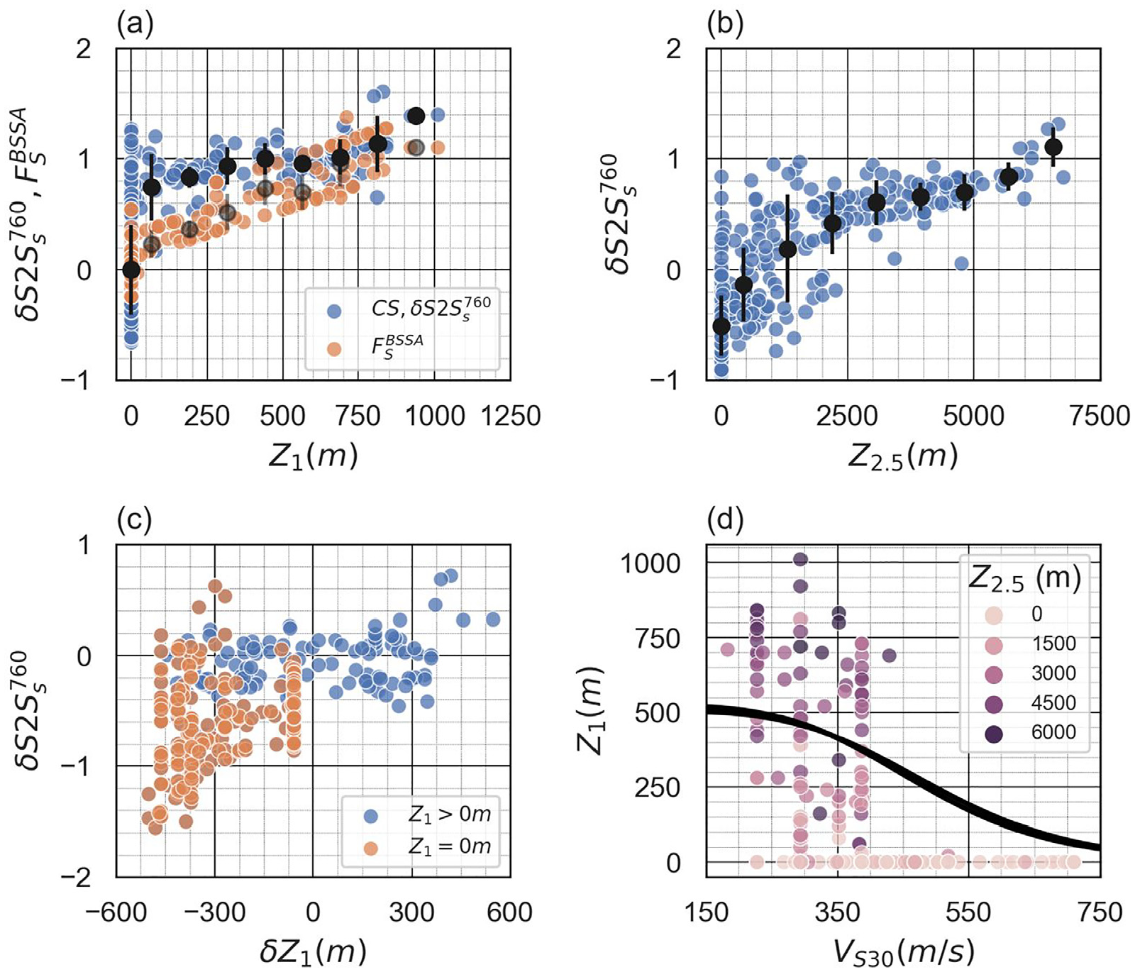
Simulation-based site terms from uniform reference condition residuals ( $\delta S2S_s^{760}=\frac{1}{N}\sum _{e=1}^N{R}_{\mathrm{es}}^{760}$ ) as a function of basin and differential depth and the relationship between shallow site conditions as shear-wave velocity in the upper 30 m ( $V_{S30}$ ) and basin depths ( $Z_1$ ). (a) Site terms ( $T=2\mathrm{s}$ ), computed for reference $V_{S30}$ site conditions ( $V_{S30}=760\mathrm{m}/\mathrm{s}$ ), as a function of $Z_1$ from the CyberShake data set are compared with the linear site ( $F_{\mathrm{lin}}$ ) and basin terms ( $f_b$ ) from Boore et al. (2014; BSSA), $F_S^{\mathrm{BSSA}}=[F_{\mathrm{lin}}\left(V_{S30}^{\mathrm{site}}\right)+f_b(Z_1^{\mathrm{site}})]-[F_{\mathrm{lin}}(V_{S30}=760\mathrm{m}/\mathrm{s})+f_b(Z_1={\mu }_{Z_1}(V_{S30}=760\mathrm{m}/\mathrm{s}))]$ . Binned mean values and standard deviations are plotted as black (CyberShake) and gray (BSSA) circles with error bars. (b) Site terms ( $T=2\mathrm{s}$ ), computed for reference $V_{S30}$ site conditions ( $V_{S30}=760\mathrm{m}/\mathrm{s}$ ), as a function of $Z_{2.5}$ . (c) Site terms ( $T=2\mathrm{s}$ ) computed for site-specific $V_{S30}$ as a function of differential depth ( $\delta Z_1$ ). (d) The relationship between $V_{S30}$ and $Z_1$ for sites in the CyberShake data set are compared with the prediction of Chiou and Youngs (2014). Symbol colors depict $Z_{2.5}$ values at each site.

Many sites outside of the modeled basins in southern California have high near-surface seismic velocities, including sites with $Z_1=0\mathrm{m}$ , and we interpret the amplifications observed in the CyberShake data to result from the high impedance contrast across the basin boundary at shallow depths (Figure 2a and c). Figure 2 presents the effects of the use of out-of-basin and in-basin sites in the basin-amplification models. Figure 2a depicts the scaling of uniform reference condition site terms ( $\delta S2S_s^{760}$ ) with $Z_1$ from the simulations, compared with the predicted site-response terms (i.e. $F_{\mathrm{lin}}+F_b$ ) from BSSA14; although the slopes of the site terms are comparable, the simulations show far greater amplification—about a factor of two—occurring between sites with $Z_1\approx 0\mathrm{m}$ and $Z_1\approx 100\mathrm{m}$ than are predicted by the empirical GMM. The scaling of the uniform reference condition site terms with $Z_{2.5}$ does not show a similar rapid increase, which may be due to smoother variations of $Z_{2.5}$ in the seismic velocity model compared to the $Z_1$ variations (Figure 2b). Plots of the uniform reference condition site terms as a function of differential depth ( $\delta Z_1$ ) show that uniform reference condition site terms on average have negative values and negative differential depths. The high seismic velocities outside of the basins are probably unphysical for most sites and would have the effect of reducing ground motions at out-of-basin sites, thus causing artificially high apparent amplifications between sites within and outside of the basins. To avoid the biasing effects on the basin-depth scaling models from sites with potentially unphysical $Z_1$ values, we restrict our analysis to sites with $Z_1>50\mathrm{m}$ . Incorporation of these sites in the development of the basin-depth scaling models will affect the slope, which we interpret to be an artifact of unphysical site conditions (Figure 2c). We choose $Z_1>50\mathrm{m}$ for selecting data because it approximately corresponds to the reference $Z_1$ value for sites with $V_{S30}=760\mathrm{m}/\mathrm{s}$ . We find that small changes to this value ( $0\le Z_1<50\mathrm{m}$ ) have a negligible effect on basin-depth scaling models because this data criterion primarily removes sites with $Z_1=0\mathrm{m}$ . Application of this threshold to the 336 sites of the CyberShake data set leaves 98 sites for the basin-depth scaling analysis within the basins of southern California.

Functional forms of the basin-depth scaling models

The four GMMs use different parameterizations for the basin-depth scaling, and we adopt these parameterizations for the simulation-based basin-depth scaling models.

Differential depths for NGA-West-2 GMMs

Due to the correlation between $V_{S30}$ and $Z_1$ —and the resulting collinearity that therefore arises in predicting site response with both parameters—three of the GMMs (ASK14, BSSA14, and CY14) use a centered form of the $Z_1$ parameter that removes the average $Z_1$ as a function of $V_{S30}$ (i.e. $Z_{1,\mathrm{ref}}(V_{S30})$ ):

$$\delta Z_{1,\mathrm{ASK}14}=\ln (Z_1+0.01)-\ln (Z_{1,\mathrm{ref}}^{\mathrm{ASK}14}\left(V_{S30}\right)+0.01)$$

(7)

$$\delta Z_{1,\mathrm{BSSA}14}=Z_1-Z_{1,\mathrm{ref}}^{\mathrm{CY}14}(V_{S30})$$

(8)

$$\delta Z_{1,\mathrm{CY}14}=Z_1-Z_{1,\mathrm{ref}}^{\mathrm{CY}14}(V_{S30})$$

(9)

The $\delta Z_1$ parameter is often referred to as “differential depth.” Reference $Z_{1,\mathrm{ref}}(V_{S30})$ values for California sites are provided in the relationships by ASK14 and CY14. The GMM of CB14 directly uses the $Z_{2.5}$ basin-depth parameter and does not apply a centering correction.

Allowance for a constant offset in the raw ground-motion residuals: C_SIM

For all GMMs, we solve for a constant offset between the simulated ground motions and the centered basin-depth scaling models. Following Sung and Abrahamson (2022), we refer to the constant offset for each reference GMM as $C_{\mathrm{SIM}}$ . This parameter is different than the $c_0^{\mathrm{SIM}}$ parameters of Equations 1 to 4, which are used in the forward calculation. Offsets correspond to the average difference between the simulated ground motions and the prediction from the empirical GMM at sites where there are no additional basin-depth effects (i.e. $\delta Z_1=0\mathrm{km}$ or $1<Z_{2.5}<3\mathrm{km}$ ). These offsets may be caused by differences in the level of radiated seismic energy from the source, differences in average crustal amplification effects (e.g. from differences in seismic velocity structure), or other unknown causes.

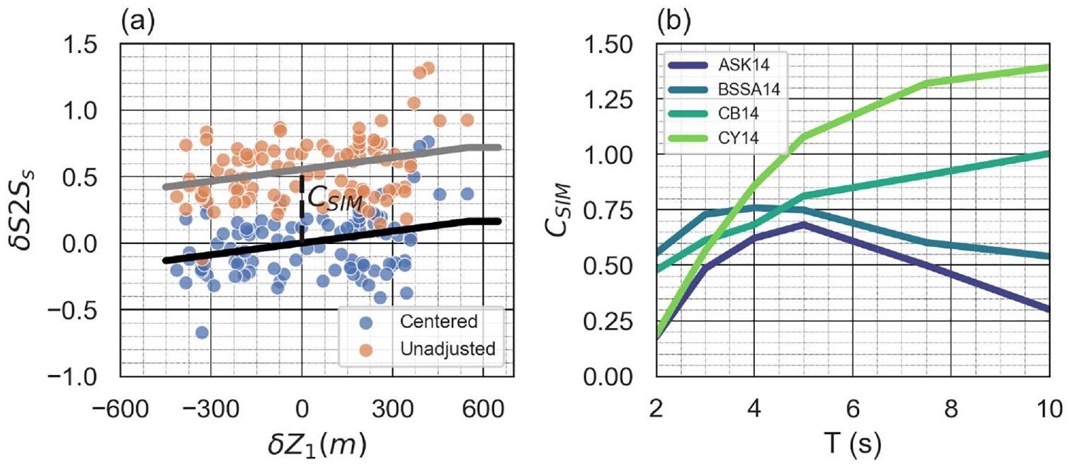
Figure 3a depicts an example calculation of the $C_{\mathrm{SIM}}$ parameter. The regression fit to the uncentered residuals—which correspond to the ground-motion residuals computed from Equation 5—results in nonzero values at $\delta Z_1=0$ (and at $1\le Z_{2.5}\le 3\mathrm{km}$ , for the $Z_{2.5}$ -based GMM); the value of the fit at $\delta Z_1=0$ is defined as $C_{\mathrm{SIM}}$ . The centered residuals or site terms ( $\delta S2S^{\prime }$ ) correspond to the ground-motion residuals adjusted by $C_{\mathrm{SIM}}$ ( $\delta S2S^{\prime }=\delta S2S-C_{\mathrm{SIM}}$ ). We use this naming because these residuals are “centered” on the GMM and thus have basin-depth scaling models that are zero-valued at $\delta Z_1=0$ .

Figure 3.

Centering of simulated ground on the parametric form of the ground-motion model (GMM) basin terms. (a) An example of computed and adjusted ground motions, and corresponding fits to the Boore et al. (2014) basin-depth scaling model, is depicted at 5-s period. The $C_{\mathrm{SIM}}$ parameter is defined as the offset of the site terms at zero-valued differential depth ( $\delta Z_1=0$ ). For the $Z_{2.5}$ -based GMM (Campbell and Bozorgnia, 2014), the $C_{\mathrm{SIM}}$ term is defined as the offset of the ground motions in the $1\le Z_{2.5}\le 3$ km depth range. (b) Variations in the $C_{\mathrm{SIM}}$ parameters from the four GMMs as a function of oscillator period (T).

Basin-depth scaling models for NGA-West-2 GMMs

We make the following minor modifications to the basin-depth functional forms provided by the GMM developers. For ASK14, we only estimate basin-depth scaling coefficients for $200<V_{S30}\le 300\mathrm{and}300<V_{S30}\le 500\mathrm{m}/\mathrm{s}$ because there is only one site for which $V_{S30}\le 200\mathrm{m}/\mathrm{s}$ and no basin sites for $V_{S30}>500\mathrm{m}/\mathrm{s}$ . For BSSA14, we allow the “corner depth” ( $\delta Z_{1,c}^{\mathrm{BSSA}14}$ ), which defines the piecewise-linear intervals, to be determined in the regression rather than specified by the functional form; for cases where the corner depth exceeds the maximum value of $\delta Z_1$ in the data set, we set $\delta Z_{1,c}^{\mathrm{BSSA}14}=550\mathrm{m}$ . For CB14, we do not estimate basin-depth scaling for shallow basin sites (i.e. at $Z_{2.5}<1\mathrm{km}$ ) because basin amplifications in the US National Seismic Hazard Model (NSHM) (Petersen et al., 2020; Powers et al., 2021) have only been applied within deep basins. The modified basin-depth scaling models are given by:

$$f_{b,\mathrm{CS}}^{\mathrm{ASK}14}(\delta Z_1^{\mathrm{ASK}14})=\{\begin{array}{c}\multicolumn{1}{c}{c_{200-300}^{\mathrm{ASK}14}\delta Z_1^{\mathrm{ASK}14},200<V_{S30}\le 300\mathrm{m}/\mathrm{s}}\\ \multicolumn{1}{c}{c_{300-500}^{\mathrm{ASK}14}\delta Z_1^{\mathrm{ASK}14},300<V_{S30}\le 500\mathrm{m}/\mathrm{s}}\end{array}$$

(10)

$$f_{b,\mathrm{CS}}^{\mathrm{BSSA}14}\left(\delta Z_1^{\mathrm{BSSA}14}\right)=\{\begin{array}{c}{c}_0^{\mathrm{BSSA}14}\delta Z_1^{\mathrm{BSSA}14},\delta Z_1^{\mathrm{BSSA}14}\le \delta Z_{1,c}^{\mathrm{BSSA}14}\hfill \\ c_1^{\mathrm{BSSA}14},\delta Z_1^{\mathrm{BSSA}14}>\delta Z_{1,c}^{\mathrm{BSSA}14}\hfill \end{array}$$

(11)

$$f_{b,\mathrm{CS}}^{\mathrm{CB}14}\left(Z_{2.5}\right)=\{\begin{array}{c}0,1<Z_{2.5}<3\mathrm{km}\hfill \\ c^{\mathrm{CB}14}{e}^{-0.75}[1-{\mathrm{e}}^{0.25({\mathrm{Z}}_{2.5}-3)}],Z_{2.5}\ge 3\mathrm{km}\hfill \end{array}$$

(12)

$$f_{b,\mathrm{CS}}^{\mathrm{CY}14}\left(\delta Z_1^{\mathrm{CY}14}\right)=c_0^{\mathrm{CY}14}(1-e^{-\frac{\delta Z_1^{\mathrm{CY}14}}{c_1^{\mathrm{CY}14}}})$$

(13)

We fit these models to the site terms (Equation 6), allowing for a constant offset ( $C_{\mathrm{SIM}}$ ) between the simulations and the GMM functional forms:

$$\delta S2S_s=f_{b,\mathrm{Sim}}+C_{\mathrm{SIM}}$$

(14)

Results and discussion

We present the development of the basin-depth scaling models by addressing the methods for adjusting (or “centering”) the simulated ground motions, evaluating the effect of the use of $V_{S30}$ values from site-specific estimates or from the minimum shear-wave velocity of the simulations. Then, we present the basin term fits, evaluate options for a constant adjustment to the final basin terms, and compare the recommended basin terms with the empirical GMMs.

Constant offset between simulations and GMMs ( $C_{\mathrm{SIM}}$ ) and treatment of $V_{S30}$

Constant offset terms $C_{\mathrm{SIM}}$ —defined as the difference of the simulated ground motions at zero-valued differential depth ( $\delta Z_1$ ) or within the $1\le Z_{2.5}<3\mathrm{km}$ depth range—vary substantially between the four GMMs. An example of the constant offset for “centered” and “uncentered” ground-motion residuals from the BSSA14 GMM is depicted in Figure 3a. In all cases offsets are positive, indicating that the simulated ground motions are higher than the GMM predictions (Figure 3b). The constant offset terms are predominantly lower at 2-s period and diverge between the different GMMs at longer periods (T > 5 s). Basin-depth scaling models are fit to the offset-corrected residuals ( $\delta S2S_s^{\prime }=\delta S2S_s-C_{\mathrm{SIM}}$ ).

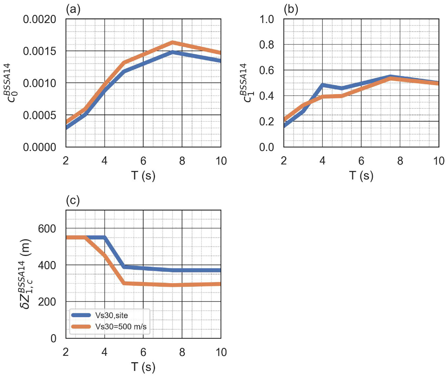
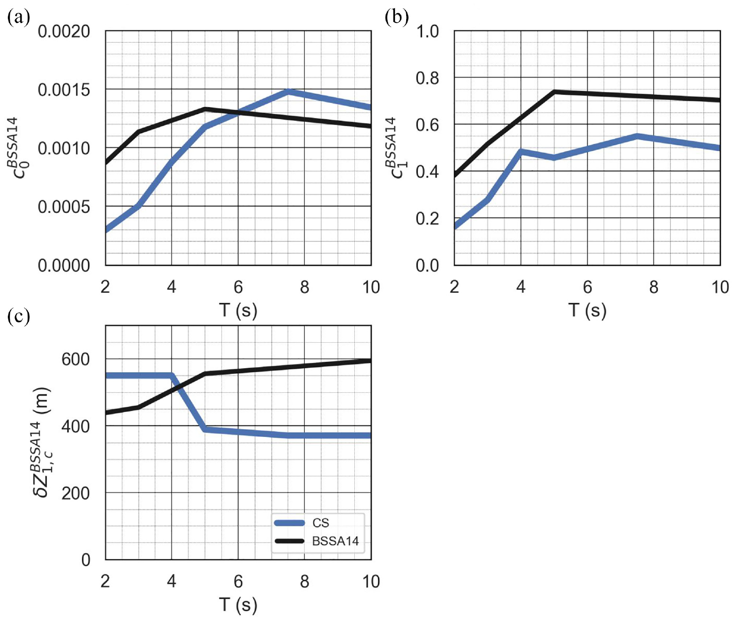
We evaluate the effects of the site-specific and uniform $V_{S30}$ values on the basin term by developing models that use both sets of site parameters. Minimal differences arise in the coefficients of basin-depth scaling models. Figure 4 depicts the values of the BSSA14 basin-depth scaling model computed from ground-motion residuals with $V_{S30}$ being site-specific or set to a uniform value of 500 m/s. Following the centering of the ground-motion residuals through the $C_{\mathrm{SIM}}$ parameter, the coefficients corresponding to the slope parameter show minor discrepancies. At periods less than about 4 s, the coefficients are highly similar. At periods greater than about 4 s, the coefficients derived from the use of uniform $V_{S30}$ values are slightly higher. Maximum amplifications and the corner depth defining the two intervals of the piecewise function from the two approaches are also similar.

Figure 4.

Effect of use of site-specific and uniform values of the time-averaged shear-wave velocity in the upper 30 m ( $V_{S30}$ ) for basin-depth scaling models, using Boore et al. (2014) as the reference ground-motion model. Model coefficients were computed from ground-motion residuals that used site-specific $V_{S30}$ values (“ $V_{S30}$ , site”) and for a uniform $V_{S30}=500\mathrm{m}/\mathrm{s}$ and are plotted as a function of oscillator period (T). (a) Coefficients correspond to the slope ( $c_0^{\mathrm{BSSA}14}$ ), (b) maximum (log) amplification ( $c_1^{\mathrm{BSSA}14}$ ), and (c) corner depth ( $\delta Z_1^{\mathrm{BSSA}14}$ ).

The minor difference between the slope parameters can be explained by differences in the site conditions (i.e. $V_{S30}$ ) of underlying simulated data. Mean $V_{S30}$ of sites in the CyberShake project is 317 m/s, which is not highly dissimilar from the uniform $V_{S30}$ value used in the calculations, although the differences in $V_{S30}$ correspond to long-period (2–10 s) ground-motion differences of about 30%–50% from the NGA-West-2 GMMs. Because lower $V_{S30}$ values correspond to greater site response in the linear $V_{S30}$ -scaling models of the NGA-West-2 GMMs, the use of site-specific $V_{S30}$ values for computing residuals results in smaller ground-motion residuals, on average. It is unexpected that this effect is not readily apparent at periods below 5 s because the $V_{S30}$ models exhibit stronger scaling at periods near 1 s. Consequently, the differences in $V_{S30}$ have a greater effect at periods less than 5 s, although this appears not to substantially affect the slopes of the basin-depth scaling models. Following centering of the simulated ground motions through the $C_{\mathrm{SIM}}$ term, the basin-depth scaling parameters from the two treatments of $V_{S30}$ are highly similar, and the choice of treatment of $V_{S30}$ for the CyberShake data set is not critical for the development of basin terms. Although we only examine the effects on basin-depth scaling parameters from BSSA14, the $V_{S30}$ scaling models from the four NGA-West-2 GMMs are similar, and we assume similar sensitivity of the fit models from use of site-specific or uniform $V_{S30}$ .

Details of the gridding in the 3D simulations may further explain the similarity of the results from the uniform-condition and site-specific-condition analyses. The thickness of the uppermost (free-surface boundary) grid cells in the CyberShake simulations is 50 m, meaning that there is uniform shear-wave velocity from the surface to 50 m depth. Because $V_{S50}=V_{S30}$ for this imposed condition, the effective $V_{S30}$ values of the simulations—or the values of $V_{S30}$ that would best explain the ground-motion amplitudes—may be lower than $V_{S,\min }$ .

We proceed using the basin-depth scaling models calculated with site-specific $V_{S30}$ values. We choose the site-specific approach for this study because we view the predictive ability of $V_{S30}$ , particularly at longer periods, to result from its statistical correlation with deeper structure. Despite the absence of shear-wave velocities less than a minimum threshold in the 3D simulations (i.e. $V_{S,\min }=500\mathrm{m}/\mathrm{s}$ for CyberShake), there is evidence that deeper seismic velocity structures control longer-period ground motions. For example, Rodgers et al. (2019) find minor effects of the minimum shear-velocity on ground motions with periods above about 2 s. The treatment of $V_{S30}$ for computing basin terms for reference GMMs remains an open question and may be more important for cases where greater differences exist between $V_{S,\min }$ and the $V_{S30}$ of basin sites.

Basin-depth scaling models from CyberShake simulations

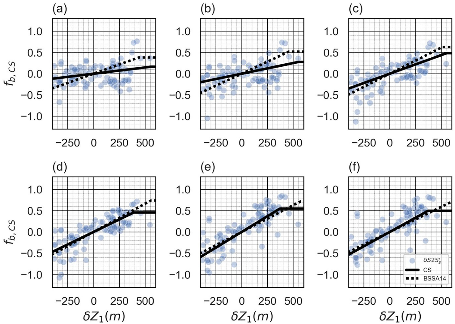
Basin-depth scaling parameters for each GMM are estimated by linear (ASK14) and nonlinear least-squares fits (BSSA14, CB14, CY14), depending on the functional form of the basin models. Example fits of the basin-depth scaling models for the BSSA14 reference model are given in Figure 5. Underlying site terms indicate variations in the strength of the basin-depth scaling with period, with relatively weaker basin-depth scaling at shorter periods ( $T=2,3\mathrm{s}$ ) and relatively stronger scaling at longer periods compared to the empirical GMM.

Figure 5.

Example fits of basin-depth scaling model from Boore et al. (2014) to CyberShake ground motions, $f_{b,\mathrm{CS}}$ plotted as a function of differential depth $\delta Z_1$ . Panels correspond to oscillator periods of (a) T = 2 s, (b) T = 3 s, (c) T = 4 s, (d) T = 5 s, (e) T = 7.5 s, and (f) T = 10 s. Solid lines correspond to the CyberShake-derived basin term, while dashed lines correspond to the basin term of the empirical ground-motion model.

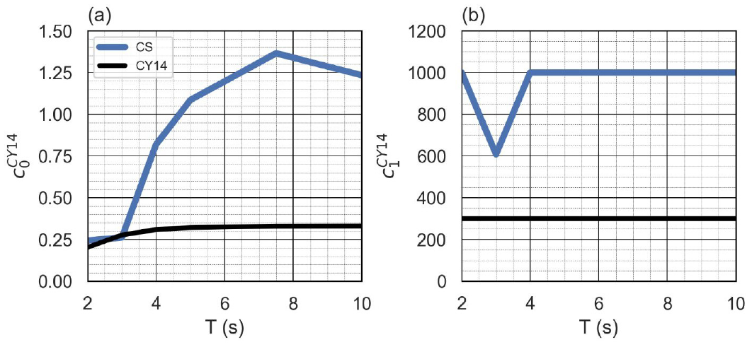
Despite differences in the ways that the empirical GMMs parameterize the basin terms, there are consistent patterns between the simulations and empirical basin terms. Coefficients for the simulation basin-depth scaling models are summarized in Figures 6 to 9, and fits to the GMMs are presented in Figures 5 and 10 to 12, along with comparisons of the basin-depth scaling models from the empirical models. For the GMMs from ASK14, BSSA14, and CB14 (Figures 6 to 8), the slope parameters from the simulations and empirical models cross at intermediate periods ( $3\le T\le 6\mathrm{s}$ ), with shallower slopes from the simulations at shorter periods. Overall, the simulation-derived slope parameters exhibit greater variation as a function of period than what is prescribed by the empirical models, and the simulation-derived slope coefficients exhibit monotonic increases with period for $2\le T\le 7.5\mathrm{s}$ . For CY14 (Figure 9), we observe similar behavior at periods of 3 s and less, with shallower (weaker) scaling of the ground motions with basin depth than is described by the empirical basin model. At longer periods, the simulation-derived basin terms indicate stronger basin-depth scaling than the empirical model. The notch in the $c_1$ parameter at 3 s period likely results from trade-offs between the $c_0$ and $c_1$ parameters and could be constrained in the regression.

Figure 6.

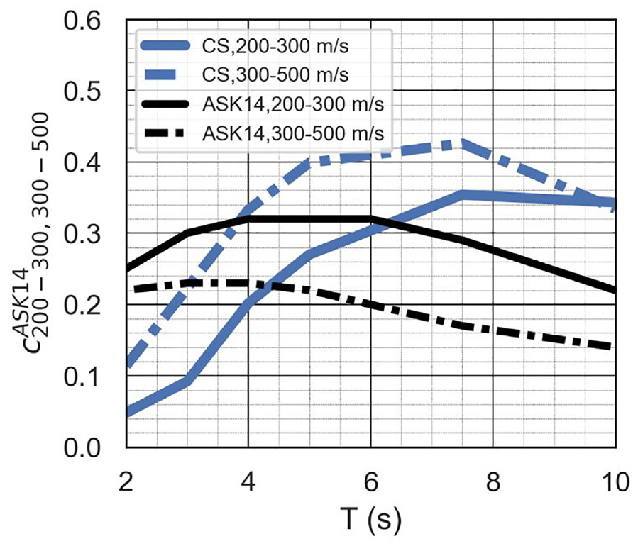
Summary of simulated and empirical basin-depth scaling models using the Abrahamson et al. (2014; ASK14) parameterization for the basin term. Coefficients from the CyberShake (CS)-derived models are depicted by blue lines, and the empirical ground-motion model coefficients are depicted with black lines and are plotted as a function of oscillator period (T). The time-averaged shear-wave velocity in the upper 30 m $(V_{S30})$ -dependent coefficients of the ASK14 basin terms are depicted by solid lines for $200<V_{S30}\le 300\mathrm{m}/\mathrm{s}$ and dashed lines for $300<V_{S30}\le 500\mathrm{m}/\mathrm{s}$ .

Figure 7.

Summary of simulated and empirical basin-depth scaling models using the Boore et al., 2014 (BSSA14) parameterization for the basin term. Coefficients from the CyberShake (CS)-derived models are depicted by blue lines, and the empirical ground-motion model coefficients are depicted with black lines and are plotted as a function of oscillator period (T). Coefficients correspond to (a) the slope ( $c_0^{\mathrm{BSSA}14}$ ), (b) maximum (log) amplification ( $c_1^{\mathrm{BSSA}14}$ ), and (c) corner depth ( $\delta Z_1^{\mathrm{BSSA}14}$ ).

Figure 8.

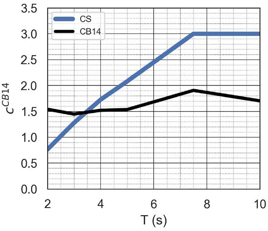
Summary of simulated and empirical basin-depth scaling models using the Campbell and Bozorgnia (2014; CB14) parameterization for the basin term. Coefficients from the CyberShake (CS)-derived models are depicted by blue lines, and the empirical ground-motion model coefficients are depicted with black lines and are plotted as a function of oscillator period (T).

Figure 9.

Summary of simulated and empirical basin-depth scaling models using the Chiou and Youngs (2014; CY14) parameterization for the basin term: for the (a) $c_0^{\mathrm{CY}14}$ parameter and (b) $c_1^{\mathrm{CY}14}$ parameter. Coefficients from the CyberShake (CS)-derived models are depicted by blue lines, and the empirical ground-motion model coefficients are depicted with black lines and are plotted as a function of oscillator period (T).

Figure 10.

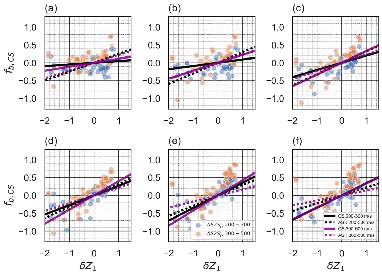
Comparison of fits of basin-depth scaling model from Abrahamson et al. (2014; ASK14) to CyberShake (CS) site terms, $f_{b,\mathrm{CS}}$ plotted as a function of differential depth $\delta Z_1$ . Basin terms for ASK14 are developed for binned site conditions of $200\le V_{S30}<300\mathrm{m}/\mathrm{s}$ (blue symbols) and $300\le V_{S30}<500\mathrm{m}/\mathrm{s}$ (orange symbols), where V_S30 is the shear-wave velocity in the upper 30 m. Panels correspond to oscillator periods of (a) T = 2 s, (b) T = 3 s, (c) T = 4 s, (d) T = 5 s, (e) T = 7.5 s, and (f) T = 10 s.

Figure 11.

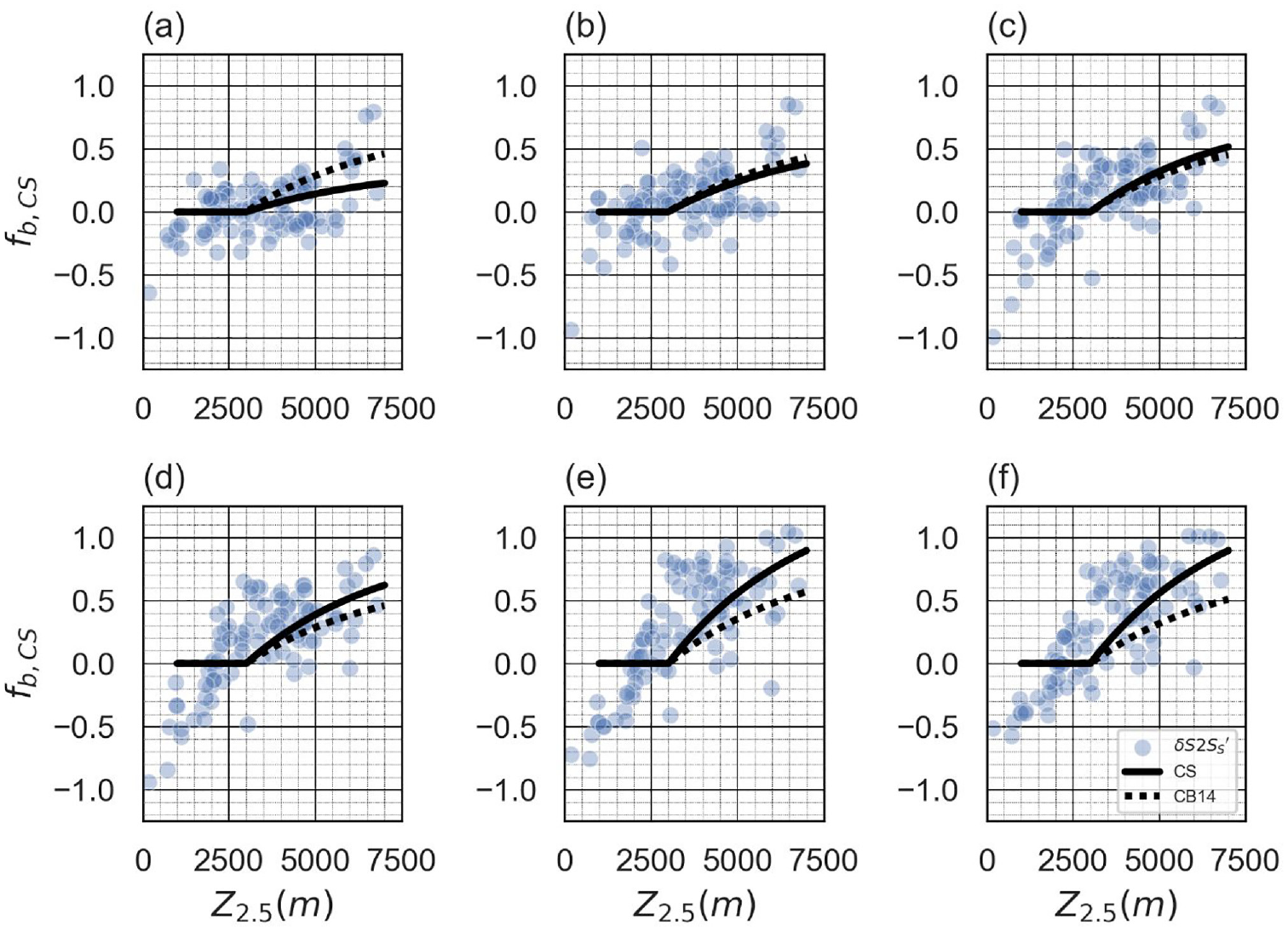
Comparison of fits of basin-depth scaling model from Campbell and Bozorgnia (2014; CB14) to CyberShake (CS) site terms, $f_{b,\mathrm{CS}}$ plotted as a function of depth to the $V_S=2.5\mathrm{km}/\mathrm{s}$ isosurface, $Z_{2.5}$ . Panels correspond to oscillator periods of (a) T = 2 s, (b) T = 3 s, (c) T = 4 s, (d) T = 5 s, (e) T = 7.5 s, and (f) T = 10 s.

Figure 12.

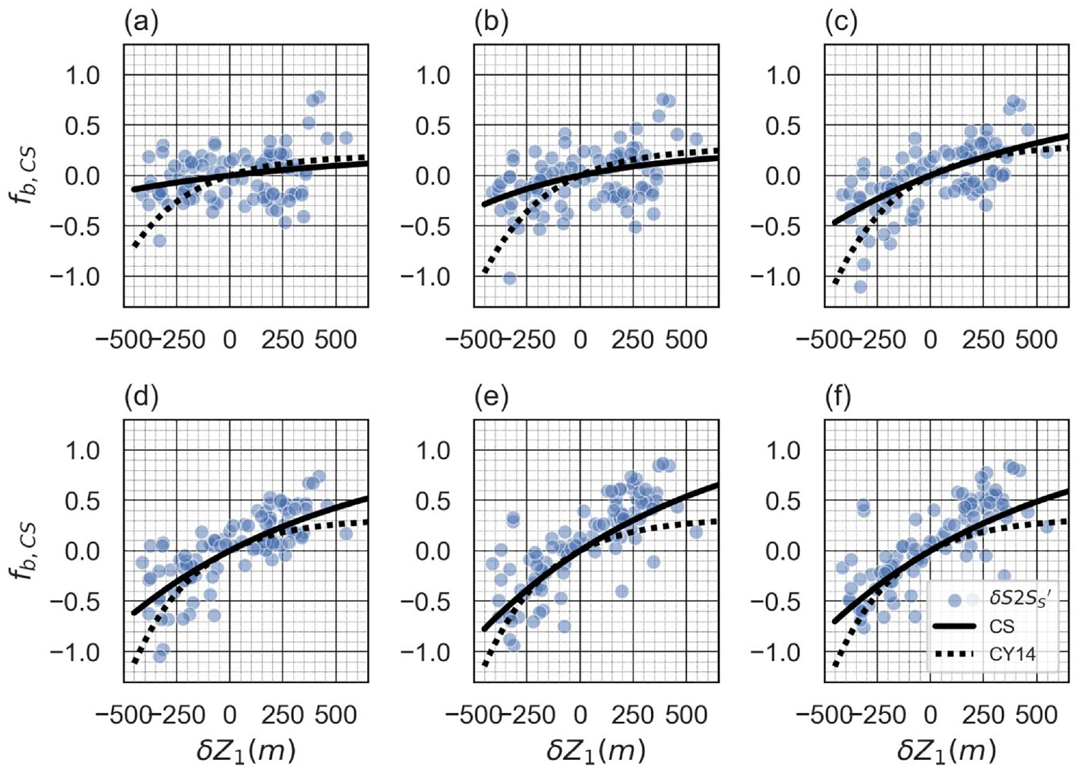
Comparison of fits of basin-depth scaling model from Chiou and Youngs (2014; CY14) to CyberShake site terms (CS) and the empirical basin terms (CY14), $f_{b,\mathrm{CS}}$ plotted as a function of differential depth $\delta Z_1$ . Panels correspond to oscillator periods of (a) T = 2 s, (b) T = 3 s, (c) T = 4 s, (d) T = 5 s, (e) T = 7.5 s, and (f) T = 10 s.

The differences in basin-depth scaling from the simulated and observed ground motions remain unexplained, and understanding these factors is important for advancing the use of simulation-derived basin terms and for improving the simulations. One potential explanation for the period-dependent discrepancy is that the seismic velocity structure, as a function of depth, is on-average smoother than what exists in the region. Shallow basin structure is known to affect ground-shaking features (e.g. Lai et al., 2020) and might explain the period-dependent differences between the simulations and observations. Too smooth seismic velocity structure could have resulted from the tomographic inversions that produced the current structural model, by minimizing impedance contrasts in the shallow part of the model and shifting lower seismic velocities to deeper depths within the basin (Lee et al., 2014). Alternatively, the simulations may capture important average effects from large-magnitude earthquakes—such as directivity-basin coupling—which predominate the simulation data set but only make up a small fraction of the empirical data set (e.g. Denolle et al., 2014; Wang and Jordan, 2014). Further studies to determine the causes of the differences identified here would be beneficial.

Constant adjustment to the simulation-derived basin term, $c_0^{\mathrm{SIM}}$

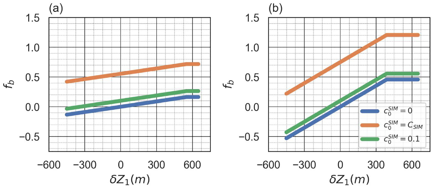
The centering of simulated ground motions on the basin-depth scaling functions of the empirical GMMs removes information about the absolute level of ground motion from the simulations, and we explore several options for adjusting the absolute ground-motion level, $c_0^{\mathrm{SIM}}$ , for seismic hazards applications. Note that the $c_0^{\mathrm{SIM}}$ parameter serves to scale the absolute ground-motion level for forward calculation, while the $C_{\mathrm{SIM}}$ parameter serves to center the simulated ground motions on the GMMs. Two options are proposed by Sung and Abrahamson (2022) for an ergodic model with a basin term derived from 3D simulations in the Pacific Northwest. For the first option, they propose the adjustment $c_0^{\mathrm{SIM}}=0$ , which corresponds to the version of the GMM that is centered on the empirical GMM at a differential depth of zero ( $\delta Z_1=0$ ). For the second option, they propose $c_0^{\mathrm{SIM}}=C_{\mathrm{SIM}}$ , which constrains the simulation-derived GMM to match the simulated ground motions at zero differential depth (i.e. $\delta Z_1=0$ ). A third option for adjusting the basin term comes from recent observations by Nweke et al. (2022) in southern California, which indicate that the centering of the BSSA14 GMM at differential depths of zero for all sites shows an amplification for three distinct geomorphic provinces (valleys, mountains/hills, and basin/basin-edges); within sedimentary basins and near basin edges, they find additional (natural log) amplifications of ∼0.1 at periods $T\ge 2\mathrm{s}$ . We refer to the Nweke et al. (2022) factors as “empirically adjusted.” Examples of the three options for the constant adjustment factor are depicted in Figure 13.

Figure 13.

Example effect of additional adjustment factors to simulation-derived basin-depth scaling models for the Boore et al. (2014) reference ground-motion model at oscillator periods of (a) 2 s and (b) 5 s. Additional adjustment factors are derived from the unadjusted simulated ground motions ( $c_0^{\mathrm{SIM}}=C_{\mathrm{SIM}}$ ), from the centered ground motions ( $c_0^{\mathrm{SIM}}=0$ ), and from Nweke et al. (2022; $c_0^{\mathrm{SIM}}=0.1$ ). Basin-depth terms ( $f_b$ ) are plotted with natural log units and are plotted as a function of differential depth $\delta Z_1$ .

The choice of the additional adjustment has important implications for ground-motion prediction because the range of (natural log) values of $C_{\mathrm{SIM}}$ can exceed 0.7 (as shown in Figure 13), which corresponds to a factor of ∼2. Differences in the empirically adjusted ( $c_0^{\mathrm{SIM}}=0.1$ ) and centered ( $c_0^{\mathrm{SIM}}=0$ ) ground motions are far smaller and correspond to an increase of about 10%. Lacking explanation or justification for the higher ground motions from the simulations, we disfavor direct use of the amplitudes from the simulated ground motions (i.e. $c_0^{\mathrm{SIM}}=C_{\mathrm{SIM}}$ ). The higher ground motions may be due to interactions between the rupture generator and 3D seismic velocity model or other factors that should be reconciled prior to direct use of the simulated amplitudes.

We favor use of the empirically adjusted factors for the basin-depth scaling terms for which they are appropriate (i.e. $\delta Z_1$ -based models) and use of the centered basin-depth scaling terms for other GMMs (i.e. $Z_{2.5}$ -based models). This is our preferred choice because the approach separates the basin effects from some of the assumptions and modeling details of the 3D simulations that affect the absolute ground motions, and the approach is consistent with recent observational data on ground motions within the sedimentary basins of southern California (Nweke et al., 2022). Although the Nweke et al. (2022) factors were computed for the BSSA14 GMM, the $\delta Z_1$ -based GMMs use similar reference $Z_1$ values, and we expect the empirical adjustments from these GMMs to be similar. In the absence of adjustment factors derived from other GMMs, we apply the empirical adjustment factor to all $\delta Z_1$ -based GMMs. Whether there are similar empirical adjustments for the $Z_{2.5}$ -based GMM is unknown, we recommend use of the centered form of the basin-depth model (i.e. $c_0^{\mathrm{SIM}}=0$ ) for this GMM. The preferred basin-depth scaling models from CyberShake are depicted in Figure 14.

Figure 14.

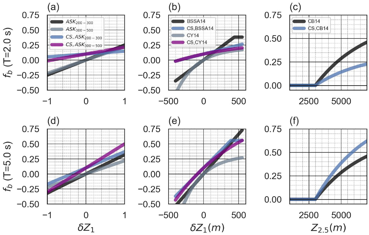
Comparison of basin-depth scaling models ( $f_b$ ) from the CyberShake simulated ground models and from empirical ground-motion models (GMMs) presented at oscillator periods of (a to c) 2 s and (d to f) 5 s. We present only the preferred adjustments for each GMM— $c_0^{\mathrm{SIM}}=0.1$ for the differential-depth-based ( $\delta Z_1$ ) GMMs and $c_0^{\mathrm{SIM}}=0$ for the depth to $V_S=2.5\mathrm{km}/\mathrm{s},Z_{2.5}$ -based GMM. CyberShake-derived basin-depth scaling models are labeled by “CS,” and the basin-depth scaling models from the empirical GMMs are labeled by the abbreviations ASK14 (Abrahamson et al., 2014), BSSA14 (Boore et al., 2014), CB14 (Campbell and Bozorgnia, 2014), and CY14 (Chiou and Youngs, 2014).

Recommended simulation-derived basin terms and effects on ground motion

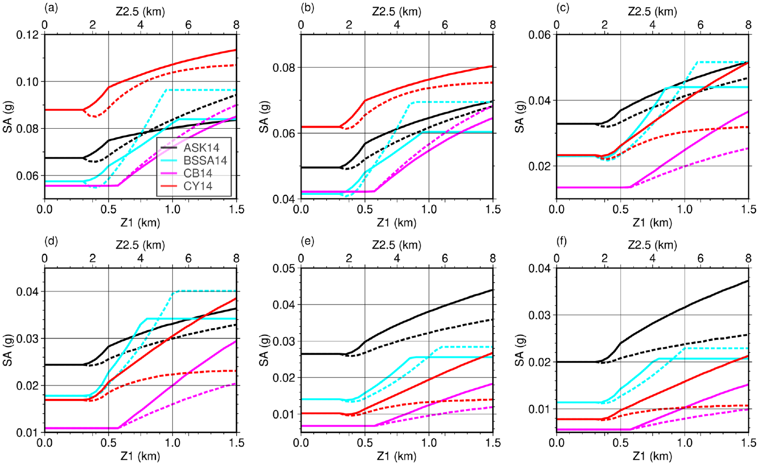
Behavior of the simulation-derived basin-depth scaling models is further examined by implementing the recommended models into the US Geological Survey’s seismic hazard code, nshmp-haz (Powers et al., 2022). The 2018 US NSHM limited basin effects to the amplifying effects of deep basins (Petersen et al., 2020; Powers et al., 2021, 2022). Examples of the simulation-derived basin terms at $V_{S30}=260\mathrm{and}360\mathrm{m}/\mathrm{s}$ are depicted for three oscillator periods (T = 2, 5, 10 s) in Figure 15. The basin terms parameterized by $Z_1$ and $Z_{2.5}$ are plotted together. Basin-depth scaling exhibits the period-dependent differences in the simulation-derived and empirical basin-depth scaling models, with shallower slopes at the shorter periods (T∼2, 3 s) and steeper slopes at longer oscillator periods. Furthermore, the recommended empirical adjustment factors ( $c_0^{\mathrm{SIM}}=0.1$ ) for the $Z_1$ -based GMMs affect ground motions at all basin depths but are particularly prominent at shallow basin sites for shorter-period ground motions. The effect of the tapering function that was implemented in the 2018 NSHM at shallow basin depths causes mild relative deamplifications at sites $Z_1<500\mathrm{m}$ .

Figure 15.

Comparison of basin-depth scaling for empirical and CyberShake-derived basin models at multiple periods (T = 2, 5, 10 s) and time-averaged shear-wave velocity in the upper 30 m ( $V_{S30}$ ) values plotted as a function of depths to $V_S=1.0\left(Z_1\right)\mathrm{and}2.5\mathrm{km}/\mathrm{s}(Z_{2.5})$ . Solid lines correspond to the simulation-derived basin models, and dashed lines correspond to the empirical GMM basin models. Periods are depicted in columns (a and d) T = 2 s, (b and e) T = 5 s, (c and f) T = 10 s, and site conditions are depicted in rows (a to c) $V_{S30}=260\mathrm{m}/\mathrm{s}$ and (d to f) $V_{S30}=360\mathrm{m}/\mathrm{s}$ .

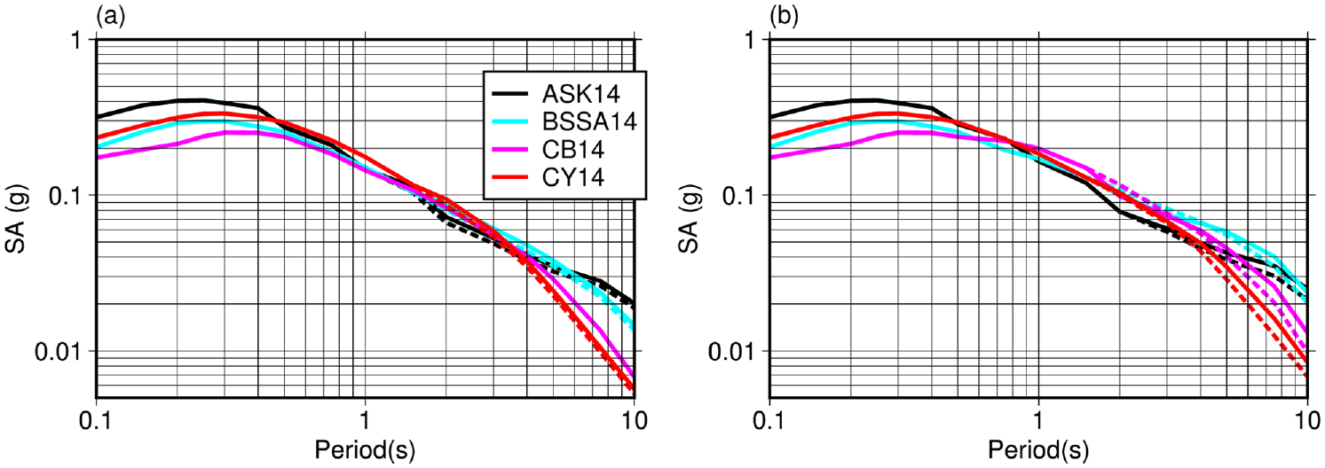
Response spectra for hypothetical shallow ( $\delta Z_1\approx 0.0\mathrm{m}$ ) and deep-basin sites further show the effects of the simulation-derived basin terms (Figure 16). For these scenarios and site conditions, we present response spectra for an $M_{W}7.5$ event, recorded at distances of 50 km ( $R_{\mathrm{RUP}}=50\mathrm{km},R_{\mathrm{JB}}=50\mathrm{km},R_X=50\mathrm{km}$ ) for site conditions corresponding to $V_{S30}=260\mathrm{m}/\mathrm{s}$ . Basin depths differentiate the shallow ( $Z_1=0.45\mathrm{km},Z_{2.5}=3\mathrm{km}$ ) and deep ( $Z_1=0.8\mathrm{km},Z_{2.5}=5.5\mathrm{km}$ ) sites and are consistent with values for the basins of southern California modeled by the CyberShake simulations.

Figure 16.

Comparison of median response spectra from the empirical GMMs (dashed lines) and CyberShake-adjusted GMMs (solid lines), for example, site conditions corresponding to (a) shallow basin depths, $Z_1=0.45\mathrm{km},Z_{2.5}=3\mathrm{km}$ (i.e. $\delta Z_1\approx 0\mathrm{km}$ ) and a (b) deeper basin site, $Z_1=0.8\mathrm{km},Z_{2.5}=5.5\mathrm{km}$ . Scenario ground motions were computed for $M_W$  = 7.5, $R_{\mathrm{RUP}}=50\mathrm{km}$ , $R_{\mathrm{JB}}=50\mathrm{km}$ , $R_X=50\mathrm{km}$ , width = 15 km, dip = 90°, $Z_{\mathrm{hyp}}=7.5\mathrm{km}$ , $Z_{\mathrm{TOR}}=0\mathrm{km}$ . Reference $Z_1$ values from NGA-West-2 GMMs are $Z_{1,\mathrm{ref}}^{\mathrm{ASK}14}(V_{S30}=260\mathrm{m}/\mathrm{s})=0.475\mathrm{km},Z_{1,\mathrm{ref}}^{\mathrm{BSSA}14}(V_{S30}=260\mathrm{m}/\mathrm{s})=0.485\mathrm{km}$ , and $Z_{1,\mathrm{ref}}^{\mathrm{CY}14}(V_{S30}=260\mathrm{m}/\mathrm{s})=0.485\mathrm{km}$ .

Conclusion

We develop basin-depth scaling models from the simulated ground motions of the SCEC CyberShake project for use with the empirical NGA-West-2 GMMs, using the functional forms of each GMM and solving for updated parameters for the basin terms. We explore two options for the treatment of $V_{S30}$ in the calculation of the ground-motion residuals and find that the choice of site-specific or uniform ( ${\mathrm{V}}_{\mathrm{S}30}=500\mathrm{m}/\mathrm{s}$ ) values has a minor effect on the parameters of the basin terms, relative to other choices involved in the development of the models. The differences are likely offset by the similarity between the mean $V_{S30}$ of CyberShake sites and the value used for the uniform $V_{S30}$ ; other simulated ground-motion data sets may yield more substantial effects on the basin terms from these approaches. The simulation-derived basin-depth scaling models exhibit period-dependent deviations from the empirical models, with weaker, shorter-period ( $T\lesssim 4\mathrm{s}$ ) depth scaling and stronger, longer-period depth scaling. The causes of the discrepancy in the strength of depth scaling are not understood but may be explained by details of the seismic velocity model or by important, unmodeled features of basin amplification from large-magnitude earthquakes. Finally, we explore alternative constant offsets for the implementation of the basin terms, including a centered version (no offset), direct use of the simulated ground motions, and use of an adjustment factor from a recent observational study (i.e. empirically adjusted). We recommend the use of the empirical adjustment for the $Z_1$ -based GMMs and use of the centered version for the $Z_{2.5}$ -based GMM. The basin-depth models developed here may be considered for use in seismic hazards assessments in the Greater Los Angeles region, and particularly within the deeper basins of the region. Although further improvements to hazards assessments from ground-motion simulations are likely to be achieved in future years, this work describes simulation-derived achievements that may be implemented in current projects and may be considered for site-specific and regional-scale studies. Approaches to integrating features from ground-motions simulations with empirical GMMs—such as the methods outlined here—are likely to be among the promising ways to make use of advancements in computational seismology for seismic hazards applications in the coming years. Continued development of methods to integrate simulations and GMMs may improve the accuracy and uncertainty quantification for earthquake hazards assessments.