Sage Journals: Discover world-class research

Abstract

Assessing post-seismic damage on an urban/regional scale remains relatively difficult owing to the significant amount of time and resources required to acquire information and conduct a building-by-building seismic damage assessment. However, the application of new methods based on artificial intelligence, combined with the increasingly systematic availability of field surveys of post-seismic damage, has provided new perspectives for urban/regional seismic damage assessment. This study analyzes the effectiveness and relevance of a number of machine learning techniques for analyzing spatially distributed seismic damage after an earthquake at the regional scale. The basic structural parameters of a portfolio of buildings and the post-earthquake damage surveyed after the Nepal 2015 earthquake are analyzed and combined with macro-seismic intensity values provided by the United States Geological Survey ShakeMap tool. Among the methods considered, the random forest regression model provides the best damage predictions for specified ground motion intensity values and structural parameters. For traffic-light-based damage classification (three classes: green-, amber-, and red-tagged buildings based on post-earthquake damage grade), a mean accuracy of 0.68 is obtained. This study shows that restricting learning to basic features of buildings (i.e. number of stories, height, plinth area, and age), which could be readily available from authoritative databases (e.g. national census) or field-surveyed databases, yields a reliable prediction of building damage (4 features/3 damage grade accuracy: 0.64).

Keywords

Machine learning 2015 Gorkha Nepal earthquake post-earthquake building-damage data building damage prediction regional and urban scale damage assessment

Introduction

Earthquakes may not occur frequently; however, they contribute significantly to the physical and social consequences of natural hazards. From 1990 to 2017, the consequences of earthquakes represent an annual average of approximately US$34.7 billion (OECD, 2018). Information regarding the estimated extent and spatial distribution of potential seismic damage within a built environment is crucial for decision makers, emergency planners, insurers, and reinsurers (e.g. Bommer and Crowley, 2006; Earle et al., 2009; Ranf et al., 2007; Riedel and Guéguen, 2018). The level of detail, methods, and tools required for the assessment are conditioned by the objectives to be achieved (Erdik et al., 2011). The estimation of potential damage could be obtained through fragility or vulnerability modeling. Seismic fragility or vulnerability modeling is the crossing of hazard, exposure, and fragility/vulnerability component (Crowley et al., 2019). The exposure-related component provides information regarding the built environment, including vulnerability class, function, reconstruction cost, and spatial distribution. The hazard-related component defines the ground-shaking potential in a region of interest based on a probabilistic seismic hazard assessment or from a deterministic rupture scenario. Finally, the vulnerability/fragility-related component relates hazards with exposure to determine the likelihood of potential damage (Silva et al., 2018). Many advanced empirical methods have been developed for seismic vulnerability assessment (e.g. FEMA, 2003; Guéguen et al., 2007; Hancilar et al., 2010, 2012; Lagomarsino and Giovinazzi, 2006; Milutinovic and Trendafiloski, 2003; Silva et al., 2014), based on field surveys of building parameters in relation to standardized building typologies, which are associated with the vulnerability or fragility functions for a specified seismic intensity measurement. The application of these damage assessment methods for rapid damage assessment in regional or urban scale is still challenging because the acquisition of building features and the application of classical methods is time- and resources-consuming on urban or regional scale.

Over the past decade, substantial progress has been realized in the field of machine learning tools and their applications in various domains. Within the scope of this study, Riedel et al. (2015) demonstrated the capacity of the support vector machine in providing seismic vulnerability assessments at regional and national scales. As the application of conventional vulnerability assessment methods on a large scale requires information that is not readily available, they proposed assessing the ability of available data from national census for a region to estimate building vulnerabilities and modeling seismic damage for specified seismic intensities. More recent studies have demonstrated the efficiency of using machine learning techniques in seismic-risk engineering to solve the aforementioned time and resource issues (Chi et al., 2020; Hegde and Rokseth, 2020; Karmenova et al., 2020; Mangalathu et al., 2020a; Sajedi and Liang, 2020; Salehi and Burgueño, 2018; Sun, 2019; Zhang and Burton, 2019; Zhao et al., 2020). Xie et al. (2020) summarized the ongoing research on the application of machine learning methods in earthquake engineering; they concluded that the implementation of machine learning in earthquake engineering is still in its early stage and needs further investigations. Limited numbers of studies are available concerning the post-earthquake damage classification using machine learning (Harirchian et al., 2021; Mangalathu et al., 2020b; Roeslin et al., 2020; Stojadinović et al., 2022). In particular, Mangalathu et al. (2020b) tested the performance of machine learning techniques in a building damage survey performed after the 2014 South Napa earthquake and demonstrated the effectiveness of such tools in interpreting the patterns of seismic damage observed in buildings. Harirchian et al. (2021) studied the performance of different machine learning methods for damage prediction in reinforced concrete (RC) buildings. They observed reasonable damage prediction by machine learning models and suggested further investigation by considering a large number of buildings with more features to define the building vulnerability. Roeslin et al. (2020) explored the performance of different machine learning methods using 2017 Puebla-Morelos earthquake building damage data and suggested further investigation using a large number of buildings in each damage typology.

In fact, the added value of post-earthquake studies based on building-damage observations has long been recognized for its contribution in improving our understanding and validating state-of-the-art seismic-risk assessment models (Colombi et al., 2008; Del Gaudio et al., 2017, 2020; Eleftheriadou and Karabinis, 2011, 2012; Guðmundsson, 2012; Karababa and Pomonis, 2011; Spence et al., 2009). In parallel to these machine learning developments, open access to a significant amount of information describing real-estate portfolios has improved (Crowley et al., 2020), and post-earthquake building-damage surveys are now available online (Dolce et al., 2019; Loos et al., 2020; NPC, 2015a). For example, the National Planning Commission of Nepal shared a massive data survey of damaged buildings after the 7.8 M_w Nepal earthquake in 2015 (NPC, 2015a).

To prepare for the increased use of machine learning for earthquake and seismological engineering applications, combined with the increasing number of open-source data, independent studies on independent datasets and with different machine learning methods are essential to advance science in this emerging field. Unlike previous studies (e.g. Mangalathu et al., 2020b; Roeslin et al., 2020), this study herein compares the damage prediction performance of various machine learning models to explain post-earthquake seismic damage, considering two different classifications of damage and two different sets of building features, applied to the 2015 Nepal earthquake building-damage portfolio (NBDP). This dataset is first described in the second section. In the third section, we present a summary of the selected machine learning tools applied to the dataset. In the fourth section, we present and discuss the results, considering damage assessment as the target value of this study. Finally, we provide our conclusions and perspectives in the last section.

Building-damage prediction database

On 25 April 2015, a devastating 7.8 M_w earthquake struck central Nepal, with an epicentral distance of approximately 80 km northwest of Kathmandu, a hypocentral depth of 8.2 km, and a 120-km long rupture toward the east. Level VIII epicentral intensity was estimated in Nepal based on the observed damage (Martin et al., 2015). Thousands of residential buildings were damaged, resulting in 8790 fatalities and 22,300 injuries (NPC, 2015b). In addition, 31 among 75 administrative districts of Nepal were affected, with 14 districts being severely affected and declared as crisis-hit areas, and an estimated loss of around US$7 billion was reported (NPC, 2015b). The government of Nepal conducted a massive post-earthquake survey in the 11 most severely affected districts (Figure 1), excluding the Kathmandu Valley. The survey comprised a visual screening of damaged buildings by experts to map the damage in each district and to develop the NBDP database. The NBDP database comprised information regarding 762,106 buildings, each characterized by socioeconomic status, engineering properties, and damage. The damage grades were classified into five levels (5DG) that are generally used in post-earthquake surveys following the EMS-98 damage classification system:

Damage Grade 1 (DG1): Thin cracks in walls and falling of plaster or loose stones from the upper part of the building, few architectural repairs required.

Damage Grade 2 (DG2): Cracks, falling of plaster or stones in many sections, damage to non-structural parts such as chimneys, and projecting cornices, with no significant reduction in the load-bearing capacity of the building.

Damage Grade 3 (DG3): Large, extensive cracks and collapse of a small portion of non-load-bearing walls. Detachment of roof tiles, tilting or falling of chimneys, failure of individual non-structural elements such as partitions/gable walls, and delamination of stone/adobe walls. Partial reduction in the load-bearing capacity of structural members, significant repairs required.

Damage Grade 4 (DG4): Large gaps or collapse of walls and partial structural failure of floors/roofs, resulting in the building classified as dangerous.

Damage Grade 5 (DG5): Complete or near collapse.

The color scale in Figure 1 highlights the proportion of buildings tagged with DG5 in each district. In addition, a set of building parameters related to structure and environment, frequently used in empirical seismic vulnerability assessment, was assigned to each screened building for the NBDP database:

Numbers of stories: total numbers of floors above the ground surface.

Height of building: total height of the building above the ground surface measured in feet.

Building age: calculated from the date of construction to the date of the earthquake.

Plinth area: total area occupied by the building at ground floor level in square feet.

Ground slope condition: ground surface topography at the building location, considering three types of ground slope conditions, that is, flat, mild slope, and steep slope.

Roof type: three types of roofs are considered based on the material used, that is, light timber/bamboo roof, heavy timber/bamboo roof, and RC roof.

Position of building: indications of the building’s location relative to other buildings. Four types of positions are cited, that is, stand-alone, attached on one side, attached on two sides, and attached on three sides.

Construction material: 11 types of construction materials used in the superstructure are considered: adobe, stone flange, mud-mortar stone, mud-mortar brick, cement-mortar stone, cement-mortar brick, RC non-engineered, RC engineered, timber, bamboo, and others.

Figure 1.

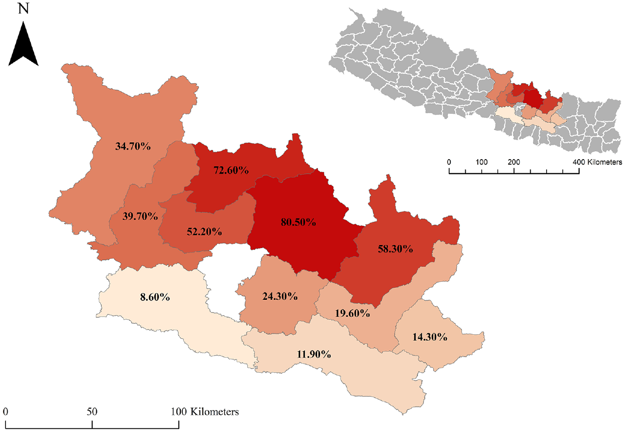
Location of the studied area and the proportion of DG5 tagged buildings (percentage indicated and highlighted by the color scale) in the 11 districts surveyed by the Nepalese authorities (NPC, 2015a).

Furthermore, in the NBDP database the geographic location of each building was assigned to a ward that belonged to a district. The ward was an elementary administrative cell. The total number of wards in 11 districts was 949. Considering building-by-building locations and the associated soil conditions, which may vary within a ward, can improve the damage prediction performance of a machine learning model (Mangalathu et al., 2020b; Roeslin et al., 2020; Stojadinović et al., 2022). However, having as objective the large-scale classification of damages (and not the classification and representation per building), and considering the macro-seismic intensities, the attribution of each building within a ward is consistent with our approach.

In a first case, all the building features contained in the NBDP database are considered in the learning phage, without any preconceived idea on their significance or possible cross-correlation. Their importance score will then be evaluated in order to know their contribution in the learning phase. In a second case, a subset of input features assumed easy to collect without significant expertise or available via authoritative national or global open databases are considered to test their damage prediction performance, without taking into account their importance.

No specific data cleaning methods were applied to the NBDP database. In the NBDP database, 12 buildings had missing damage information so they were removed from the database and 5731 buildings had missing age value so they were replaced by the average age value.

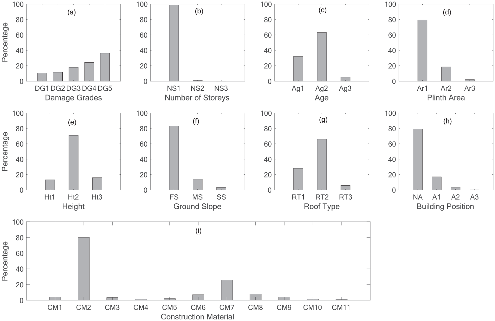
Table 1 and Figure 2 summarizes the distribution of the building parameters in the database. In the NBDP database, the distribution of the buildings per damage grade was as follows: 10.34% for DG1, 11.45% for DG2, 17.90% for DG3, 24.12% for DG4, and 36.19% for DG5. The number of stories ranged from one to nine floors, the building age ranged from 1 to 200 years, the building plinth area ranged from 70 to 5000 sq ft, and the building height was between 6 and 97 ft (approximately 2 to 30 m). The distribution of buildings based on the material used to construct the superstructure was as follows: 4.24% adobe, 80.02% mud-mortar stone, 3.51% stone flange, 1.58% cement mortar stone, 2.29% mud-mortar brick, 7.15% cement-mortar brick, 25.87% timber, 8.04% bamboo, 3.97% RC non-engineered, 1.63% RC engineered, and 1.20% other materials.

Table 1.

Distribution of different building parameters present in the Nepal earthquake building-damage portfolio database

No.	Parameters		Data type	Distribution (%)	Remarks
1	Damage Grades (DG)	DG1	Categorical	10.34	Figure 2a
		DG2		11.45
		DG3		17.90
		DG4		24.12
		DG5		36.19
2	Number ofstories	0–3 (NS1)	Numerical	98.9	Figure 2b
		3–5 (NS2)		1.04
		>5 (NS3)		0.06
3	Age (years)	0–10 (Ag1)	Numerical	32.03	Figure 2c
		10–50 (Ag2)		62.92
		>50 (Ag3)		5.05
4	Plinth area (sq ft)	0–500 (Ar1)	Numerical	79.39	Figure 2d
		500–1000 (Ar2)		18.54
		>1000 (Ar3)		2.07
5	Height (ft)	0–10 (Ht1)	Numerical	13.19	Figure 2e
		10–20 (Ht2)		70.93
		>20 (Ht3)		15.88
6	Ground slope at Building’s location	Flat slope (FS)	Categorical	82.89	Figure 2f
		Mild slope (MS)		13.87
		Steep slope (SS)		3.24
7	Roof type	Bamboo/timber heavy roof (RT1)	Categorical	28.05	Figure 2g
		Bamboo/timber light roof (RT2)		66.10
		Reinforce concrete (RT3)		5.85
8	Building position	Stand-alone (NA)	Categorical	79.32	Figure 2h
		Attached to one side (A1)		16.98
		Attached to two sides (A2)		3.53
		Attached to three sides (A3)		0.17
9	Construction material	Adobe (CM1)	Categorical	4.24	Figure 2i
		Mud-mortar stone (CM2)		80.02
		Stone-flange (CM3)		3.51
		Cement-mortar stone (CM4)		1.58
		Mud-mortar brick (CM5)		2.29
		Cement-mortar brick (CM6)		7.15
		Timber (CM7)		25.87
		Bamboo (CM8)		8.04
		Non-engineered reinforced concrete (CM9)		3.97
		Engineered reinforced concrete (CM10)		1.63
		Others (CM11)		1.20

Figure 2.

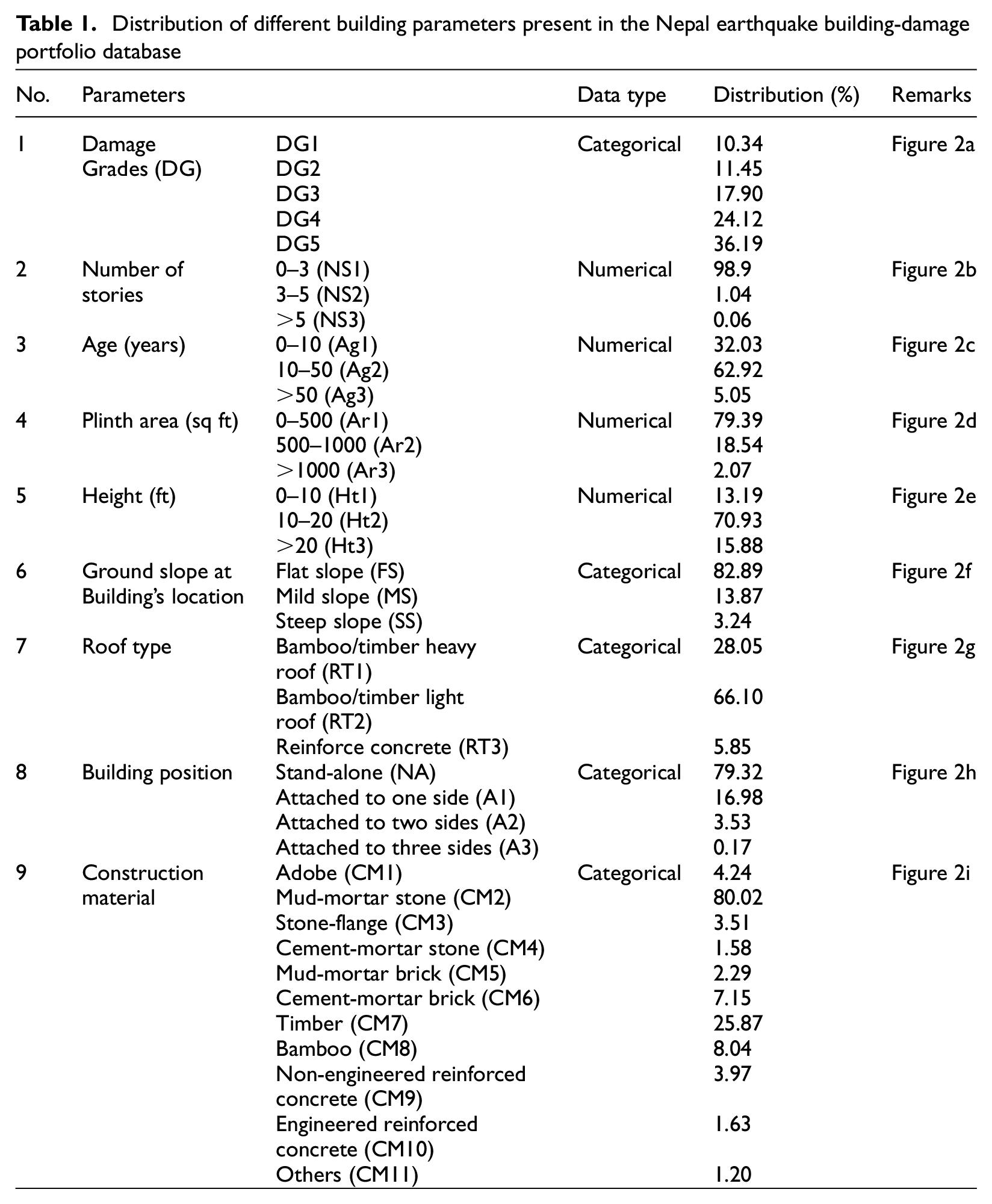
Distribution of building parameters in the whole NBDP dataset. The y-axis shows percentage and the x-axis is (a) damage grade, (b) number of stories (NS1: 0–3, NS2: 3–5, NS3: .5), (c) age (Ag1: 0–10, Ag2: 10–50, Ag3: .50), (d) plinth area (Ar1: 0500, Ar2: 500–1000, Ar3: .1000), (e) building height (Ht1: 0–10, Ht2: 10–20, Ht3: .20, in ft as contained in the original database), (f) ground slope condition at building location (FS: flat slope; MS: mild slope; SS: steep slope), (g) roof construction material (RT1: heavy bamboo/timber roof; RT2: light bamboo/timber roof; RT3: reinforced concrete), (h) position of building with respect to other buildings (A1: attached on one side; A2: attached on two sides; A3: attached on three sides; NA: stand-alone building), and (i) superstructure construction material (CM1: adobe; CM2: mud-mortar stone; CM3: stone-flange; CM4: cement-mortar stone; CM5: mud-mortar brick; CM6: cement-mortar-brick; CM7: timber; CM8: bamboo; CM9: RC non-engineered; CM10: RC engineered; CM11: other).

Additional information provided by the ShakeMap tool from the United States Geological Survey (USGS) supplied the macro-seismic intensity (MSI) field and completed the database (Wald et al., 2005). ShakeMap provides an estimate of the spatial distribution of earthquake ground-shaking intensity by combining recorded ground motions, modeled ground motions, Did You Feel It? information, and slope-v_S30-based site conditions. In recent studies requiring spatially distributed information as input ground motion, ShakeMap intensities have been successfully used to compensate for insufficient instrumental data (Del Gaudio et al., 2020; Jaiswal and Wald, 2010; Mak and Schorlemmer, 2016; Pothon et al., 2020; Silva and Horspool, 2019). The USGS ShakeMap provides the MSI value in modified Mercalli intensity scale (Figure 3a). Because the geolocalization of the buildings is available at the ward level, we computed the mean MSI value for each ward and assigned it to all the buildings located within the same ward. The MSI values ranged from 5.30 to 8.30 (Figure 3b).

Figure 3.

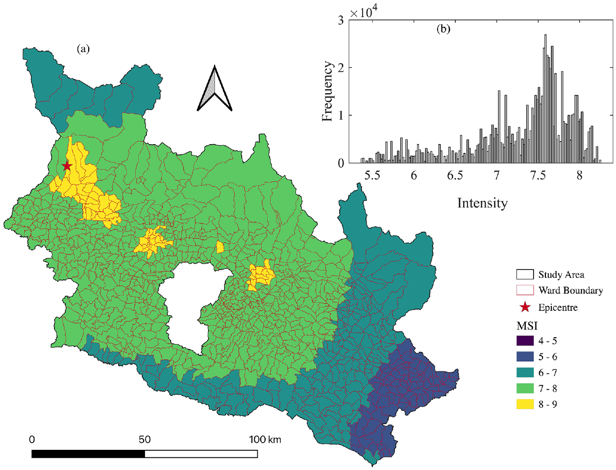
(a) Spatial distribution of the macroseismic intensity for the 7.8 Mw earthquake in 2015 obtained from the USGS ShakeMap tool and (b) distribution of the macro-seismic intensity in the database, the x-axis is the intensity value and the y-axis is the frequency.

Method

In this study, damage prediction was considered first as a classification problem. Machine learning classification involves assigning a label (or class) to categorical response variables. Damage grades (from 1 to 5) are considered categorical variables; hence, the application of classification models is recommended. In this study, we focused on two typically used classification machine learning methods, that is, random forest classification (RFC) (Breiman, 2001) and gradient boosting classification (GBC) (Friedman, 1999). However, the damage grades were ordered and can be regarded as a continuous variable to minimize misclassification errors. In this study, regression models were considered simultaneously with the damage grade as a continuous variable ranging between 1 (DG1) and 5 (DG5). Because the regression model outputs a real value between 1 and 5 and not an integer, we rounded the output (real number) to the nearest integer to plot the confusion matrix. However, the error matrices were computed without rounding the model outputs to the nearest integer. Four regression machine learning models were considered, that is, linear regression (LR) (Hastie et al., 2009), support vector regression (SVR) (Cortes and Vapnik, 1995), gradient boosting regression (GBR) (Friedman, 1999), and random forest regression (RFR) (Breiman, 2001). Using classification methods, every misclassification yields the same penalty loss, whereas regression methods penalize the relative penalty loss (i.e. difference error) by minimizing the squared loss between the true and predicted damage grades. In this study, we tested both approaches (regression and classification), and their strengths and weaknesses in terms of damage prediction were compared.

RFC/RFR and GBC/GBR are based on a set of several decision trees as base learners; this enables them to achieve greater efficiency while integrating the complexity and nonlinear interaction of the features in the dataset. LR has simple analytical and computational properties; additionally, it can easily illustrate the interpretable description of the effect of the input on the output, that is, the contribution of each feature in the model. SVR is effective in high-dimensional spaces and is extremely versatile in terms of application (i.e. it can be used for linear and polynomial models).

Hereinafter, the damage grade is defined as the target variable, and the building parameters (i.e. number of stories, height, age, plinth area, ground-slope condition, building position, roof type, and construction material) and the ground-motion intensity (MSI) are defined as the input features. A one-hot encoding technique was used to transform categorical values (i.e. construction material, position, ground slope condition, and roof type) into nominal values (Pedregosa et al., 2011). The one-hot encoding technique generates a unique binary value 1 or 0 for each categorical feature by creating a sparse matrix, which resulted in 26 input features for the model (Table 1).

The building damage dataset was randomly partitioned into three subsets. The training dataset constituted 60% of the entire dataset and was used to train the machine learning model. Meanwhile, the validation dataset constituted 20% of the entire dataset and was used to select the best model by comparing the strengths and weaknesses of the different machine learning models for damage prediction (section “Model selection”). Model optimization was performed by investigating data imbalance arising from the unequal distribution of the target features in the training dataset (section “Management of data imbalance”) and the importance of each feature in the model (section “Feature importance”). The test dataset constituted the remaining 20% of the entire dataset; it was kept hidden from the model until the final optimized model was developed. Once the optimized model was developed, the test dataset was used to test the performance of damage prediction of the optimized model (section “Damage prediction using test dataset”). The percentage distribution of each feature in the training, validation, and test dataset follows the same percentage distribution as in the entire NBDP database (Figure 2).

In this study, we used the models provided in Python using the Scikit-learn package. The performance of each model was quantified by measuring the accuracy score (percentage of correctly predicted labels) (Pedregosa et al., 2011). A high accuracy score (approximately 1) indicates the high efficacy (i.e. ability to perform a task to a satisfactory or expected degree) of the machine learning model in damage prediction. In addition, we computed the following statistical error indicators to compare the performance of each machine learning model: the mean of the absolute error (MAE) and the mean squared error (MSE). The scores of these indicators are referred to as the performance scores hereinafter. The smaller the MAE (approximately 0) and MSE (approximately 0), the higher is the efficacy of the models. We considered different metrices because we observed that one metric could not fully explain the predictive performance among classification and regression methods. For each machine learning model, the predictive performance is extremely sensitive to the model input parameters, which are known as hyperparameters. The hyperparameters of each machine learning model were tuned using a grid-search technique on the training set. Finally, computational time (time taken by each model in our personal computer, Macbook Pro 2019) is considered as one additional parameter to facilitate comparison among machine learning models.

The performance of each machine learning technique for damage prediction is presented graphically based on the distribution of errors as well as in a confusion matrix (see Figure 4). A confusion matrix presents a comparison between the true and predicted damage grades. In the confusion matrix, the value of the predicted damage grades (cell value along the row of the confusion matrix) is normalized by the total number of true damage grades. The values along the main diagonal elements of the confusion matrix indicate the recall (i.e. the number of predicted values equal to the true values) of the machine learning model. A perfect model would have ones along the main diagonal of the confusion matrix, and zero everywhere else. In the confusion matrix, the accuracy score represents the number of correctly predicted instance (sum of the diagonal terms) over the total number of instances (sum of the full matrix). Because the regression model outputs a real value between 1 and 5 and not a label, we rounded the output (real number) to the nearest integer to plot the confusion matrix. But the error matrices were computed without rounding the model outputs to the nearest whole integer.

Figure 4.

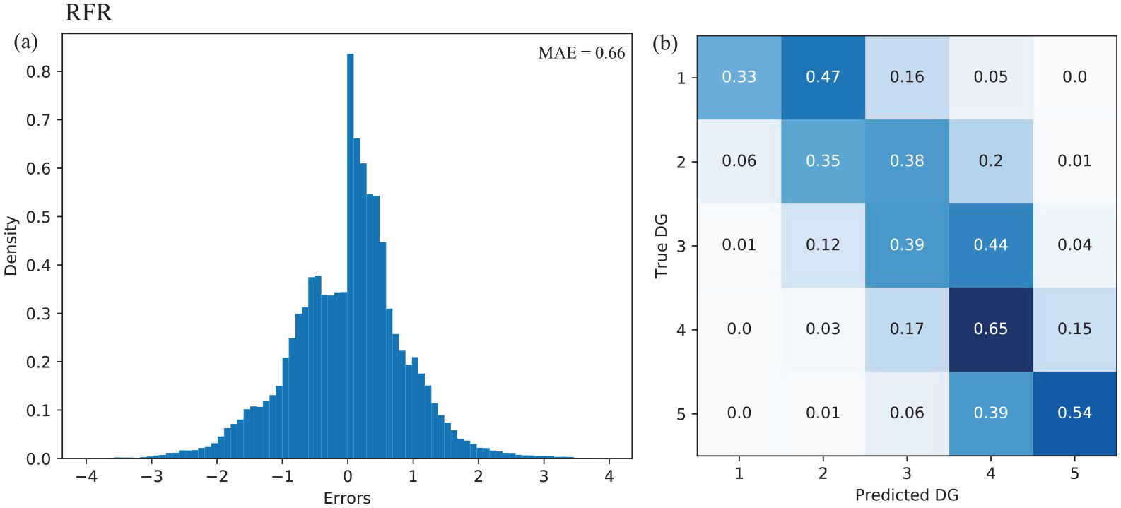
Graphical representation of the predictive performance of the random forest regression (RFR) on the validation dataset. (a) Distribution of errors between the true and predicted damage grades (DG) and corresponding MAE value. (b) DG normalized confusion matrix for the RFR model. The model outputs were rounded to the nearest whole integer to plot the confusion matrix, which is not the case to compute the error matrices.

Result

Model selection

This section summarizes the performance of damage prediction provided by the machine learning models on the validation set. The input variables, performance scores, and relative computation time for each optimized model are listed in Table 2 and Appendix 1. Within the classification model group, the GBC (MAE = 0.60) provided the best performance compared with the RFC (MAE = 0.67). The GBC and RFC yielded MSE scores of 1.05 and 1.25, respectively. The GBC (Figure 5a) and RFC (Figure 5b) provided better classification recall for the two extreme damage grades (DG1 and DG5) than for the intermediate damage grades (DG2, DG3, and DG4). For these models, the intermediate damage grades were associated with a significant misclassification, independent of the classification model. However, this result shows that the GBC and RFC models did not yield high efficacies in damage prediction. This may reflect the fact that, unlike DG1 (extremely slight damage) and DG5 (near or complete collapse), the intermediate damage grades are more subjective as well as more difficult to classify and distinguish in the field.

Table 2.

Summary of the optimized input parameters and the performance scores of different machine learning models observed on the validation dataset

Machinelearningmodel	Input parameters	Score			Computationaltime (s)
		Classificationaccuracy	Statistical
		Classificationaccuracy	MAE	MSE
LR	Default	0.30	0.86	1.14	3
SVR	C = 1 Kernel = rbf	0.43	0.77	1.09	80,900
GBR	learning rate = 0.1	0.51	0.64	0.72	875
	no_estimators = 500
	max_depth = 10
RFR	no_estimators = 1000	0.49	0.66	0.76	563
	max_depth = 20
GBC	learning rate = 0.1	0.57	0.60	1.05	8584
	no_estimators = 1000
	max_depth = 10
RFC	no_estimators = 1000	0.53	0.67	1.25	450
	max_depth = 30

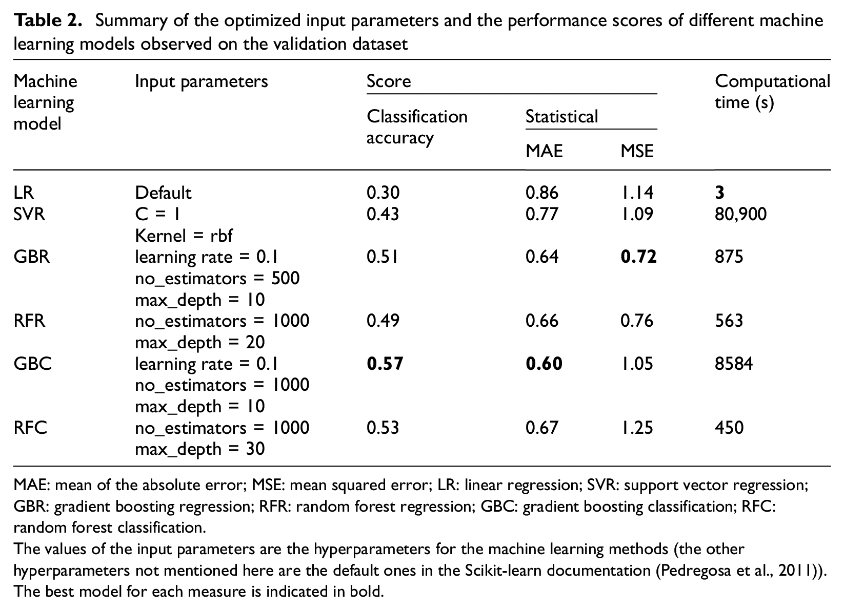
MAE: mean of the absolute error; MSE: mean squared error; LR: linear regression; SVR: support vector regression; GBR: gradient boosting regression; RFR: random forest regression; GBC: gradient boosting classification; RFC: random forest classification.

The values of the input parameters are the hyperparameters for the machine learning methods (the other hyperparameters not mentioned here are the default ones in the Scikit-learn documentation (Pedregosa et al., 2011)). The best model for each measure is indicated in bold.

Figure 5.

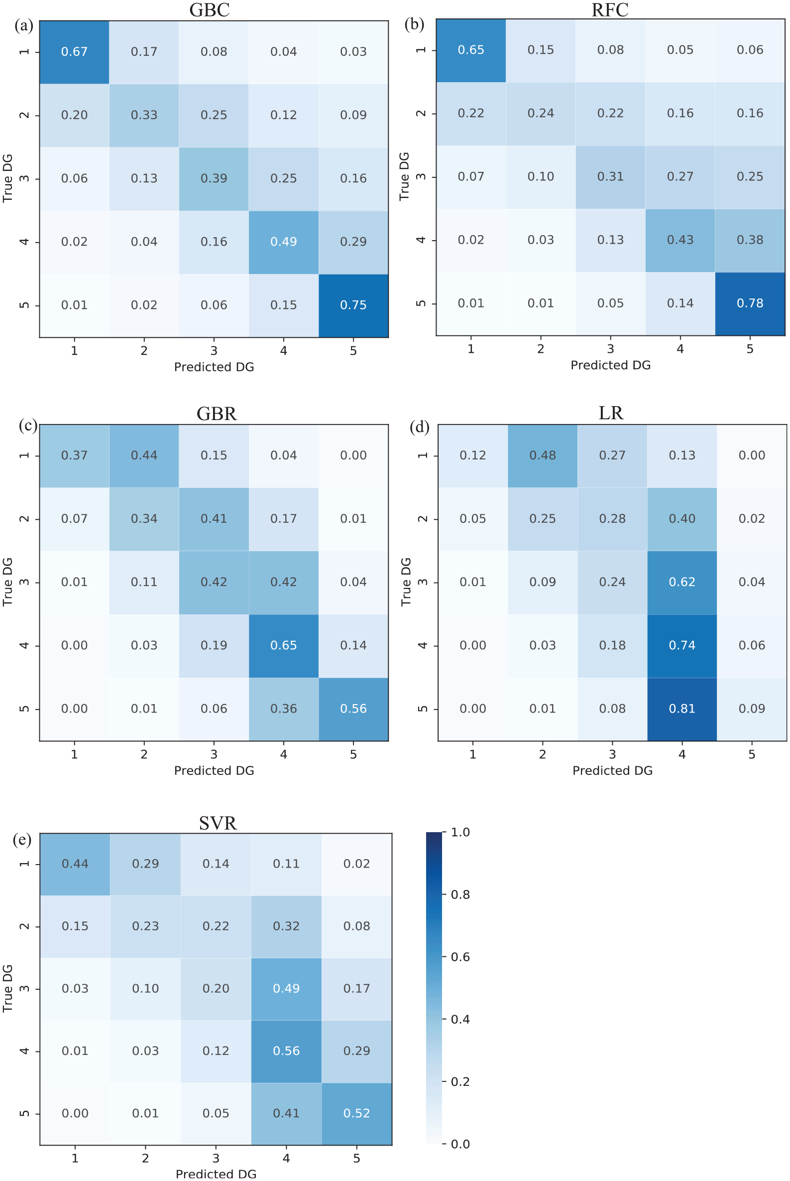
Damage grade (DG) normalized confusion matrix for (a) gradient boosting classification (GBC) model, (b) random forest classification (RFC) model, (c) gradient boosting regression (GBR) model, (d) linear regression (LR) model, and (e) support vector regression (SVR) model on the validation dataset. A color bar shows the normalized cell value for each confusion matrix.

The regression models, GBR (MAE = 0.64) and RFR (MAE = 0.66), demonstrated similar performance results, with the smallest values of MSE (GBR = 0.72; RFR = 0.76). For the RFR (Figure 4b) and GBR (Figure 5c), the predicted damage grades were similar to the ground-truth damage grades in the confusion matrix. High percentage values were observed on the diagonal of the matrix or offset by one level of damage, and they constituted 80%–95% of the total prediction in each damage grade, as shown in Figures 4b and 5c. As expected, the regression models penalized the large errors more efficiently than the GBC (Figure 5a) and RFC (Figure 5b). In addition, these methods are associated with low computational time (RFR: 563 s; GBR: 875 s, Table 2). It is noteworthy that the LR (MAE = 0.86) and SVR (MAE = 0.77) demonstrated worse performances, with a significant misclassification (LR: Figure 5d and SVR: Figure 5e) that might be due to the complexity of and nonlinear feature interactions in the dataset.

In conclusion, considering the damage-prediction task as a regression problem and using GBR/RFR machine learning models provides the best damage-prediction efficacy (see Figures 4 and 5 and Table 2). For the GBR and RFR models, the predictive performance, efficacy, and computational time were extremely sensitive to the hyperparameters. For example, the GBR model required a careful tuning of a significant number of hyperparameters, which increased the computational time compared with the RFR model. In addition, the GBR model might be less generalizable to new data owing to its possible overfitting issue and is more difficult to implement compared with the RFR model. Hence, the RFR model was used in the remainder of this study to test the damage prediction.

Management of data imbalance

The distribution of labels in the training dataset affects the performance of machine learning models (e.g., Branco et al., 2017; Estabrooks and Japkowicz, 2001; Japkowicz and Stephen, 2002). The NBDP dataset shows an unequal distribution of the damage grades, that is, the highest damage grade represents the largest fraction of the dataset (Figure 2a). This data imbalance may have affected the predictive performance of the RFR model (Figure 4). In this study, we considered some extensively adopted techniques to manage an imbalanced dataset by over and undersampling the target features (e.g. Estabrooks and Japkowicz, 2001; Japkowicz and Stephen, 2002). Undersampling is achieved by selecting an equal amount of data through random selection of a minimum number of values in each damage grade from the training dataset, whereas oversampling is achieved by replicating the minority damage grades (i.e. DG1 and DG2 in our case).

The RFR model was trained using the resampled dataset to observe its performance on the validation dataset. Figure 6 shows the performance of the RFR model after (a) undersampling and (b) oversampling. Compared with the previous model trained using an imbalanced dataset (Figure 4b), the undersampling method degraded the efficacy of the RFR model with an increase in the MAE by 9%. By oversampling, the performance yielded was similar to that of the original method (1% increase in the MAE). However, undersampling increased the recall value for the lowest damage grades (Figure 6a), that is, the recall value increased by 20%–25% for DG1 to DG3 and reduced by less than 15% for DG4 and DG5. Meanwhile, oversampling improved the recall value moderately for the lower grades without significantly affecting the recall value of the higher damage grades, for example, the DG1/DG5 recall value changed from 0.33/0.54 (Figure 4b) to 0.41/0.51 (Figure 6b), respectively. Therefore, for further studies, we plan to use the oversampling technique to address data imbalance issues such that a better estimation of the lower grades can be obtained.

Figure 6.

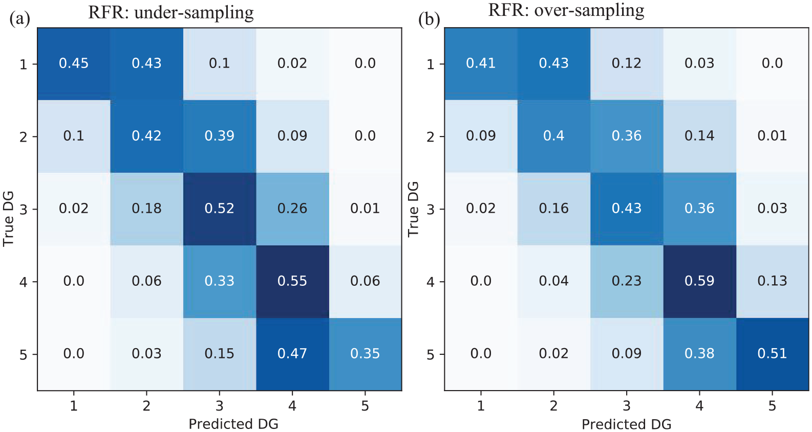
Data imbalance testing applied to the RFR model. Damage grade (DG) normalized confusion matrix for (a) undersampling and (b) oversampling techniques.

Feature importance

The importance of each input feature in the RFR damage-prediction model is analyzed in this section. In decision trees, each node is a condition for dividing the values into single characteristics such that similar values of the dependent variable appear in the same set after the division. The condition is based on impurity, which is the variance in the case of regression trees. In other words, each feature’s contribution can be measured by the average decrease in impurity using all the trees in the forest, without considering the linear separability of the data (Pedregosa et al., 2011). The significance of each feature in the model is measured in terms of the feature importance scores. The feature importance score is a value assigned to each feature in the model while a model is developed. Note also that RFR uses the bagging algorithm (randomly splitting data into smaller subsets) while developing the trees, so the correlated features may or may not be used for a particular tree. Thus, correlated features may not affect the overall predictive performance, however, it may impact the importance ranking between two correlated features, removing one of the correlated features may lower the damage predictive performance of the RFR model.

Figure 7 shows the importance score associated with each input feature considered in this study. The highest importance score (32% in Figure 7) was associated with the mud-mortar stone material. Buildings constructed using mud-mortar-stone constituted the highest proportion in our dataset (Figure 2i), and this building class was damaged severely during the Nepal earthquake, independent of the MSI. In fact, this type of building is generally associated with the most vulnerable class in most vulnerability assessment methods. The fact that the RFR identified the mud-mortar-stone feature as the most important feature in damage prediction is consistent with previous studies (Maheri et al., 2005; Sayin et al., 2013; Webster and Tolles, 1999). In addition, Figure 7 shows that, as expected, the MSIs that characterized the ground motion were one of the most significant input features for earthquake damage prediction (31%), that is, damage was first conditioned by the MSI regardless of the building parameters. Other building-related input features, such as plinth area (8%), construction age (7%), and height (5%) contributed significantly to earthquake damage prediction model; meanwhile, the other features contributed only marginally to the damage prediction model (RFR).

Figure 7.

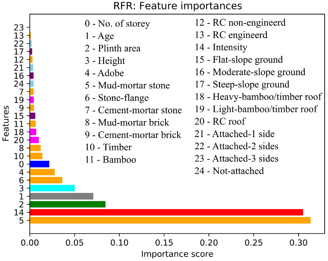
Graphical representation of the importance scores associated with the different input features considered for the RFR model. Categorical features are transformed to binary features. The features (same as in Table 1) considered in this study are on the y-axis and the x-axis is the importance score. In the figure the building features are represented by a set of colors: no. of story (blue), age (gray), plinth area (green), height (cyan), construction material (orange), MSI (red), ground slope (purple), roof type (magenta), and building’s position (sky blue).

As mentioned earlier (Table 2), a higher damage-prediction accuracy (0.49) was observed when all features were considered (MAE = 0.66). However, information regarding building construction materials is typically not easily accessible. The four basic building parameters (i.e. number of stories, age, height, and plinth area) could be easily accessible from the institutional databases (e.g. national census, national housing database) (Crowley et al., 2020; Riedel et al., 2015), from field survey, and partially available in open-source platform (e.g. OpenStreetMap (OSM) (Bennett, 2010), OpenBuildingMap (OBM) (Schorlemmer et al., 2017)). Thus, the performance of RFR model considering only the basic parameters of the building (i.e. number of stories, age, height, and plinth area) in addition to the ground-motion intensities is explored. The RFR model provided a similar level of accuracy (0.46) in damage prediction (MAE = 0.72). This result suggests that basic building parameters enable the development of satisfactory RFR models for predicting damage, and therefore earthquake losses, for the given value of ground-motion intensity (as reported by Riedel et al. (2015) and Guettiche et al. (2017) for seismic vulnerability classification using a support vector machine).

Damage prediction using test dataset

This section presents the predictive performance of the RFR model for the test dataset. The RFR model was developed for two sets of features, that is, all building parameters (i.e. full-feature setting) and the basic parameters (i.e. number of stories, age, height, plinth area, and ground-motion intensity; basic-feature setting).

The full-feature/basic-feature settings yielded MSE scores of 0.81/0.93. Confusion matrices for the full- and basic-feature settings are shown in Figure 8a and b, respectively. The main diagonals and their adjacent values are associated with a higher recall value, illustrating higher efficacy in damage prediction and a lower misclassification rate. As shown in Figures 4b and 6b, the RFR model applied to the test dataset predicted the highest damage grades (DG4/DG5) with a higher recall value, corresponding to 60%/51% and 57%/46% in the full- and basic-feature settings, respectively.

Figure 8.

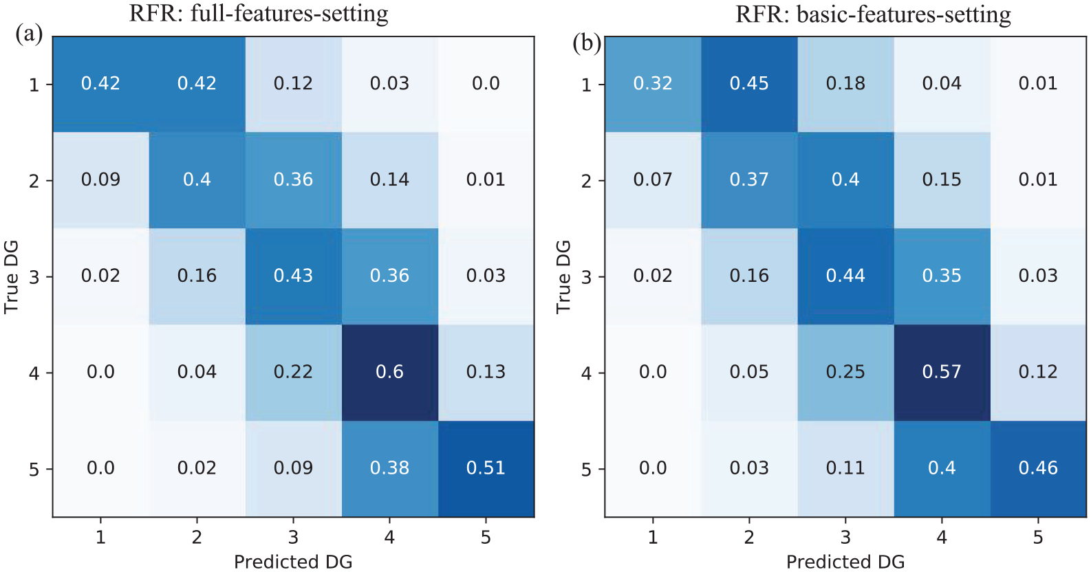
Damage grade (DG) normalized confusion matrix for (a) the full-features setting and (b) the basic-features setting observed in the test dataset.

During field observations for damage classification, it is often difficult to assign a damage level to buildings falling between two damage grades. Moreover, it is more convenient to classify damage into three categories, that is, in the same manner as using the traffic-light (TL)-based classification system (green, amber, and red) in post-earthquake emergency surveys (ATC, 2005; Bazzurro et al., 2004). Therefore, we classified the five damage grades into three categories by considering the severity of damage based on the damage grade definition (Section “Building-damage prediction database”), as follows: S (slight: DG1 + DG2), M (medium: DG3), and H (heavy: DG4 + DG5). The MSE scores for the full-feature/basic-feature settings were 0.34/0.39. Figure 9 shows the confusion matrices. The damage prediction accuracy increased significantly when the TL-based approach was used. For example, the recall values for the S/M/H damage grades were 59%/60%/73% and 51%/61%/70% for the full- and basic-feature settings, respectively.

Figure 9.

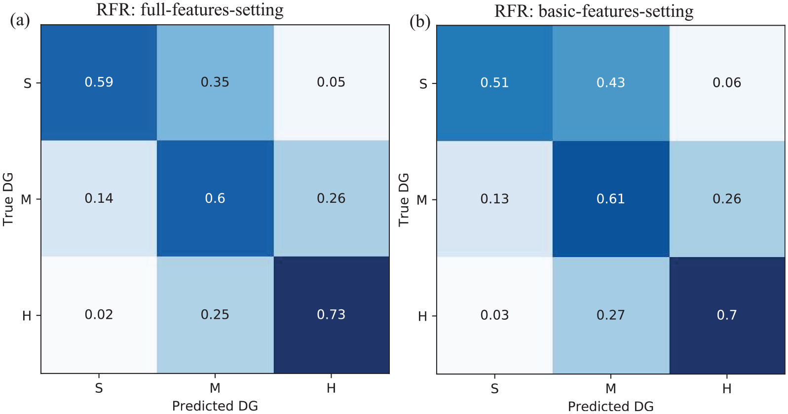
Damage grade (DG) normalized confusion matrix for (a) the full-features setting and (b) the basic-features setting in the traffic-light (TL)-based classification approach, grouping the five damage grades (DG) into three classes: slight, medium, and heavy damage grades (S, M, H).

Table 3 summarizes the MAE, and MSE scores observed with the full- and basic-feature settings. For the basic-feature setting, the values of these scores (e.g. MAE = 0.73/0.45), considering that the 5DG/TL damage scales were similar to those of the full-feature setting (e.g. MAE = 0.69/0.41). Section “Feature importance” shows that using the RFR model, a reasonable damage prediction was possible by merely considering the basic features of the buildings.

Table 3.

Summary of the performance scores for RFR model considering the test datasets for the full-features setting and basic-features setting

Features	Damage grade	Accuracy score	MAE	MSE
Full-features setting	5DG	0.49	0.69	0.81
	TL	0.68	0.41	0.34
Basic-features setting	5DG	0.46	0.73	0.93
	TL	0.64	0.45	0.39

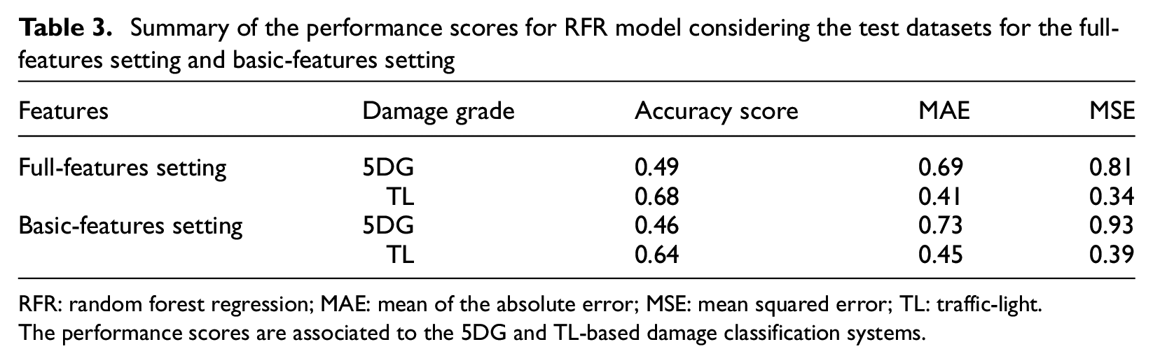
RFR: random forest regression; MAE: mean of the absolute error; MSE: mean squared error; TL: traffic-light.

The performance scores are associated to the 5DG and TL-based damage classification systems.

The results yielded by the RFR model confirmed that considering basic building features resulted in a relatively similar damage prediction efficacy compared with considering all features. The possible reason behind this is maybe the combination of these basic features is able to indirectly capture some key parameters of buildings needed to define the vulnerability, such as the building typology. The RFR model developed by considering the basic features thereby may overcome the challenges of data acquisition for vulnerability assessments as well as earthquake damage and loss prediction on the urban or regional scale.

Testing the proportioning of the dataset

We explored the damage prediction efficacy of the RFR model as a function of the amount of data in the training dataset. Figure 10 shows the performance of the method (accuracy and MSE scores) for several percentage of data in the training phase according to the test dataset (% of N_T). In this case, 100% of the original training set corresponds to 300% of N_T. For 10% of N_T, the accuracy score is 0.63/0.57 and 0.42/0.37 for TL- and 5DG-based damage classifications considering full-features/basic-features-setting, respectively. These scores are very close to the performance scores noted in Table 3. Major improvement in the damage prediction efficacy of the RFR model is achieved up to 50% of N_T. After 50%, a minor improvement is observed.

Figure 10.

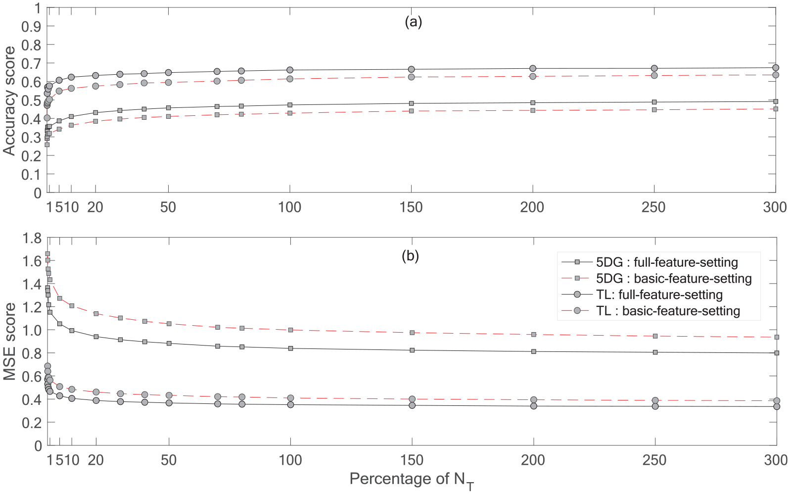
(a) Variation of the accuracy and (b) MSE of the RFR model as a function of the percentage of the whole test dataset, N_T, used for the training phase. The black-solid/red-dashed lines with the gray circle correspond to TL-based damage classification for the full-features/basic-features-setting, respectively. The black-solid/red-dash line with the gray square corresponds to 5DG-based damage classification for the full-features/basic-features-setting, respectively.

Moreover, the damage prediction efficacy of the RFR model was further improved by taking into account the geographic location of the building (ward-id in this case). For example, at 10% of N_T, the accuracy score was 0.66/0.63 and 0.47/0.44 for TL and 5DG-based damage classification at full-features/basic-features-setting, respectively.

Discussion

In this study, we investigated the efficiency of various machine learning techniques for post-earthquake seismic damage assessment using the NBDP database compiled after the 2015 7.8 M_w earthquake in Nepal. Machine learning models were trained based on a number of building characteristics and some basic parameters that contributed significantly to damage prediction performance. We tested the predictive efficacies of LR, SVR, GBC/GBR, and RFR/RFC models. For classification methods significant misclassification is observed for intermediate damage grades whereas for regression methods the predicted values were similar to the ground truth (see Figures 4 and 5 and Table 2). This could be because for classification methods every mis-classification has the same penalty loss whereas regression methods penalize the relative penalty loss (i.e. difference error) by minimizing the squared loss between true and predicted damage grades. Among these models, RFR was the most relevant model for damage prediction when applied to our dataset; it provided the best cost/benefit ratio in terms of performance and computing time. For the baseline comparison, the result obtained from the RFR model is compared with a random uniform baseline (randomly assigning damage grades following an uniform distribution) and a random stratified baseline (following the distribution of damage grades in the training set) to every input. The RFR model resulted largely higher accuracy score (0.49) compared with the random uniform baseline (0.20) and the random stratified baseline (0.25) to every input for 5DG classification. Moreover, in this case study, the RFR model demonstrated superior performance in predicting higher damage grades, which is ultimately the most pursued information for seismic damage assessment and earthquake loss reduction.

In addition, we achieved a moderate improvement in damage prediction by addressing data imbalance issues via data resampling using the RFR model. In this study, we considered an unseen test dataset to ensure the overfitting issues of the model. The error values of validation and test datasets are very similar (same 0.49 accuracy on both cases), indicating that the model did not overfit on the validation set.

However, the results herein show that considering a traffic-light damage classification and a limited number of building features, the results reach very satisfactory scores according to the objectives set: damage prediction accuracy 0.64 for basic-features setting, to be compared with Mangalathu et al. (2020b), Roslin et al. (2020), and Harirchian et al. (2021) studies that reported accuracy values of 0.66, 0.67, and 0.65, respectively, also with the random forest method. The 3-class classification model lowers the number of targets and then lowers the confusion as is often observed during damage surveys for the intermediary damage grade (e.g. between DG3 and DG4). In addition, so-called basic building features (i.e. number of stories, age, height, and plinth area) associated with ground-motion intensity provided a relevant estimate of the damage grade with a significant level of accuracy. Similar observations have also been reported by Mangalathu et al. (2020b) and Stojadinović et al. (2022) in their studies using the 2014 South Napa and 2010 Kraljevo, Serbian earthquake building damage dataset, respectively. Moreover, the RFR model trained on a relatively small amount of dataset (5%–20% of the test dataset) resulted in a reasonable estimate of damage; similar observation has been reported by Stojadinović et al. (2022).

The input ground motion used was the USGS ShakeMap intensity of the mainshock, whereas the overall quality of the NBDP database results were based on the cumulative effects of the mainshock and aftershock events, which might have affected the prediction efficacy. In addition, missing building-by-building information in the NBDP database relative to their localization and their associated site condition reduce the damage prediction efficacy of the machine learning model (Mangalathu et al., 2020b; Roeslin et al., 2020; Stojadinović et al., 2022). However, we also observed that by considering the geographic locations of buildings (ward-id in our case) slightly improved the damage prediction efficacy of the RFR model.

Finally, in Nepal, a majority of the building typology inventory collected after the 2015 earthquake holds a good match with the building typology inventory as observed in the 2011 national census (Chaulagain et al., 2015). Thus, the findings from this study seems promising to the Nepal’s exposure context. Further investigations should be carried out to strengthen these findings: after the 2015 Gorkha Nepal earthquake, national and international communities are collaborating to develop an exposure model for Nepal (Jordan, 2019).

Conclusion

To summarize, a framework for combining building parameters and earthquake building damage information collected after an earthquake event with machine learning techniques for seismic-damage assessment was presented herein. This study shows a possibility of using machine learning methods for immediate damage assessment once ground-motion information is published via operational tools, such as the USGS ShakeMap. This study shows that the building’s features (number of stories, age, floor area, height) could result in reasonable damage prediction. These basic building parameters could be available in existing institutional databases (e.g. national census, national housing database), thereby resolving data acquisition issues associated with seismic-damage assessments at the urban or regional scale.

Without anticipating how a city planner can use these results, machine learning developed on a building portfolio makes it possible to explain post-earthquake damage. One may assume that the model herein for a specific portfolio might be used to predict and represent seismic damage in another region with the same portfolio (e.g. Riedel et al., 2014) or for another characterization of the seismic hazard (Riedel et al., 2015), in an emergency situation (immediately after an earthquake if the exposure model is known) or in a planning process. This will of course have to be confirmed on another dataset, for example, consisting of a series of earthquakes affecting the same region, that is, characterized by the same portfolio of buildings. In addition, the results herein show that using a traffic-light damage classification and a limited number of building features, the results reach very satisfactory scores according to the objectives set (damage prediction accuracy 0.64 for 4 basic features/3 damage grade settings, to be compared with the studies of Mangalathu et al. (2020b), Roslin et al. (2020), and Harirchian et al. (2021) that reported accuracy values of 0.66, 0.67, and 0.65, respectively, with the random forest method).

In addition, the collection of the building exposure data is the key challenge faced by the damage assessment communities. The observed performance of machine learning considering only basic parameters, easy to collect and without requiring much technical expertise, may suggest the interest of exploring the potential of crowed-source databases (e.g. OSM/OBM) as input parameters. This approach will require validation before being able to assert it definitively, but it would solve the difficulty of considering the evolution of the building in the definition of the exposure models.

Footnotes

Appendix

Table 4.

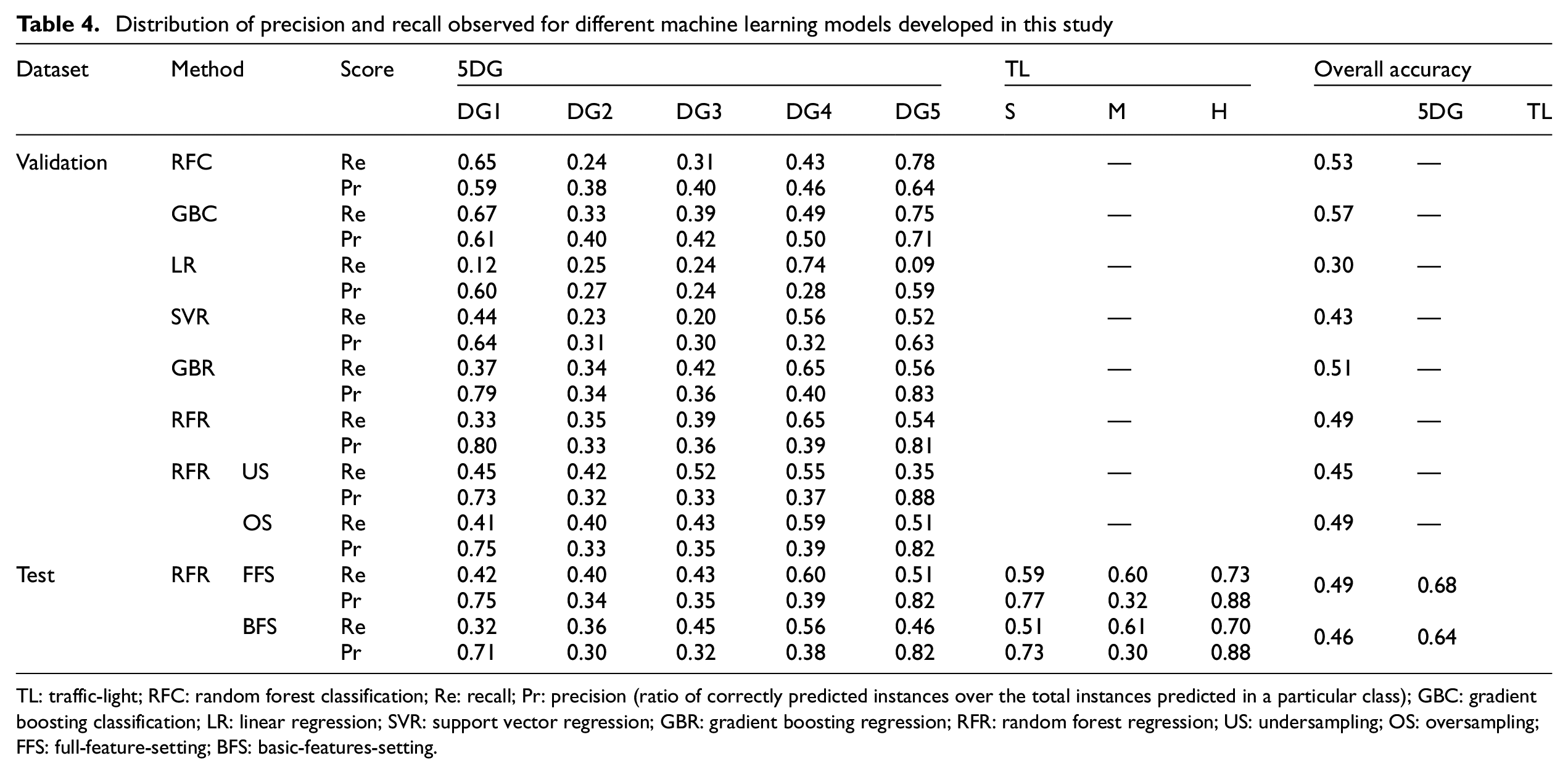
Distribution of precision and recall observed for different machine learning models developed in this study

Dataset	Method	Score	5DG					TL			Overall accuracy
			DG1	DG2	DG3	DG4	DG5	S	M	H		5DG	TL
Validation	RFC	Re	0.65	0.24	0.31	0.43	0.78		—		0.53	—
		Pr	0.59	0.38	0.40	0.46	0.64
	GBC	Re	0.67	0.33	0.39	0.49	0.75		—		0.57	—
		Pr	0.61	0.40	0.42	0.50	0.71
	LR	Re	0.12	0.25	0.24	0.74	0.09		—		0.30	—
		Pr	0.60	0.27	0.24	0.28	0.59
	SVR	Re	0.44	0.23	0.20	0.56	0.52		—		0.43	—
		Pr	0.64	0.31	0.30	0.32	0.63
	GBR	Re	0.37	0.34	0.42	0.65	0.56		—		0.51	—
		Pr	0.79	0.34	0.36	0.40	0.83
	RFR	Re	0.33	0.35	0.39	0.65	0.54		—		0.49	—
		Pr	0.80	0.33	0.36	0.39	0.81
	RFR US	Re	0.45	0.42	0.52	0.55	0.35		—		0.45	—
		Pr	0.73	0.32	0.33	0.37	0.88
	OS	Re	0.41	0.40	0.43	0.59	0.51		—		0.49	—
		Pr	0.75	0.33	0.35	0.39	0.82
Test	RFR FFS	Re	0.42	0.40	0.43	0.60	0.51	0.59	0.60	0.73	0.49	0.68
		Pr	0.75	0.34	0.35	0.39	0.82	0.77	0.32	0.88
	BFS	Re	0.32	0.36	0.45	0.56	0.46	0.51	0.61	0.70	0.46	0.64
		Pr	0.71	0.30	0.32	0.38	0.82	0.73	0.30	0.88

TL: traffic-light; RFC: random forest classification; Re: recall; Pr: precision (ratio of correctly predicted instances over the total instances predicted in a particular class); GBC: gradient boosting classification; LR: linear regression; SVR: support vector regression; GBR: gradient boosting regression; RFR: random forest regression; US: undersampling; OS: oversampling; FFS: full-feature-setting; BFS: basic-features-setting.

Acknowledgements

The authors thank Editage (www.editage.com) for English language editing. The data were provided by the National Planning Commission of Nepal ().

Declaration of conflicting interests

The author(s) declared no potential conflicts of interest with respect to the research, authorship, and/or publication of this article.

Funding

The author(s) disclosed receipt of the following financial support for the research, authorship, and/or publication of this article: This study was funded by the URBASIS-EU project (H2020-MSCA-ITN-2018, Grant No. 813137). Part of this study was supported by the Real-time earthquake rIsk reduction for a reSilient Europe (RISE) project, funded by the EU Horizon 2020 program under Grant Agreement No. 821115. P.G. thanks LabEx OSUG@2020 (Investissements d’avenir-ANR10LABX56).

ORCID iD

Subash Ghimire

Data and resources

The data used for this study are available at . The machine learning codes used were from the Scikit learn library in Python.

References

ATC (2005) ATC-20-1, Field Manual: Postearthquake Safety Evaluation of Buildings. 2nd ed. Redwood City, CA: Applied Technology Council.

Bazzurro

Cornell

Menun

, et al. (2004) Guidelines for seismic assessment of damaged buildings. In Proceedings of the 13th world conference on earthquake engineering, Vancouver, Canada. (accessed 1–6 August 2004).

Bennett

(2010) OpenStreetMap. 1st ed. Packt Publishing. Birmingham, B3 2PB.

Bommer

Crowley

(2006) The influence of ground-motion variability in earthquake loss modelling. Bulletin of Earthquake Engineering 4(3): 231–248.

Branco

Ribeiro

Torgo

, et al. (2017) SMOGN: A pre-processing approach for imbalanced regression. Proceedings of Machine Learning Research 74: 36–50.

Breiman

(2001) Random forests. Machine Learning 45: 5–32.

Chaulagain

Rodrigues

Silva

, et al. (2015) Seismic risk assessment and hazard mapping in Nepal. Natural Hazards 78(1): 583–602.

Chi

Wang

Liao

, et al. (2020) Machine learning-based seismic capability evaluation for school buildings. Automation in Construction 118: 103274.

Colombi

Borzi

Crowley

, et al. (2008) Deriving vulnerability curves using Italian earthquake damage data. Bulletin of Earthquake Engineering 6(3): 485–504.

10.

Cortes

Vapnik

(1995) Support-vector networks. Machine Learning 20: 273–297.

11.

Crowley

Daniela

Crowley

, et al. (2019) The European seismic risk model 2020 (ESRM 2020). In: 2nd International Conference on Natural Hazards and Infrastructure. Chania: Greece. (accessed 23–26 June 2019).

12.

Crowley

Despotaki

Rodrigues

, et al. (2020) Exposure model for European seismic risk assessment. Earthquake Spectra 36(Suppl. 1): 252–273.

13.

Del Gaudio

De Martino

Di Ludovico

, et al. (2017) Empirical fragility curves from damage data on RC buildings after the 2009 L’Aquila earthquake. Bulletin of Earthquake Engineering 15(4): 1425–1450.

14.

Del Gaudio

Di Ludovico

Polese

, et al. (2020) Seismic Fragility for Italian RC Buildings Based on Damage Data of the Last 50 Years. Springer. DOI: 10.1007/s10518-019-00762-6.

15.

Dolce

Speranza

Giordano

, et al. (2019) Observed damage database of past Italian earthquakes: The da.D.O. WebGIS. Bollettino di Geofisica Teorica ed Applicata 60(2): 141–164.

16.

Earle

Wald

Jaiswal

, et al. (2009) Prompt assessment of global earthquakes for response (pager): A system for rapidly determining the impact of earthquakes worldwide. US Geological Survey Open-File Report 1131: 15.

17.

Eleftheriadou

Karabinis

(2011) Development of damage probability matrices based on Greek earthquake damage data. Earthquake Engineering and Engineering Vibration 10(1): 129–141.

18.

Eleftheriadou

Karabinis

(2012) Seismic vulnerability assessment of buildings based on damage data after a near field earthquake (7 September 1999 Athens—Greece). Earthquake and Structures 3(2): 117–140.

19.

Erdik

Şeşetyan

Demircioĝlu

, et al. (2011) Rapid earthquake loss assessment after damaging earthquakes. Soil Dynamics and Earthquake Engineering 31(2): 247–266.

20.

Estabrooks

Japkowicz

(2001) A mixture-of-experts framework for learning from imbalanced data sets. In: Lecture Notes in Computer Science (Including Subseries Lecture Notes in Artificial Intelligence and Lecture Notes in Bioinformatics), vol. 2189, pp. 34–43. DOI: 10.1007/3-540-44816-0_4.

21.

FEMA (2003) Hazus –MH 2.1 multi-hazard loss estimation methodology earthquake. Available at: https://www.fema.gov/sites/default/files/2020-09/fema_hazus_earthquake-model_technicalmanual_2.1.pdf

22.

Friedman

. (1999) Greedy Function Approximation: A Gradient Boosting Machine. http://www.alford-systems.Com/doc.GreedyFuncApproxSS.Pdf

23.

Guéguen

Michel

Lecorre

(2007) A simplified approach for vulnerability assessment in moderate-to-low seismic hazard regions: Application to Grenoble (France). Bulletin of Earthquake Engineering 5(3): 467–490.

24.

Guettiche

Guéguen

Mimoune

(2017) Seismic vulnerability assessment using association rule learning: Application to the city of Constantine, Algeria. Natural Hazards 86(3): 1223–1245.

25.

Guðmundsson

(2012) Comprehensive damage analysis of buildings affected by the 2008 South Iceland earthquake. In: 15th world conference on earthquake engineering (15 WCEE). Available at: https://www.iitk.ac.in/nicee/wcee/article/WCEE2012_2384.pdf (accessed 10 June 2022).

26.

Hancilar

Taucer

Corbane

(2012) Empirical fragility assessment after the January 12, 2010 Haiti earthquake. WIT Transactions on Information and Communication Technologies 44: 353–365.

27.

Hancilar

Tuzun

Yenidogan

, et al. (2010) ELER software—A new tool for urban earthquake loss assessment. Natural Hazards and Earth System Science 10(12): 2677–2696.

28.

Harirchian

Kumari

Jadhav

, et al. (2021) A synthesized study based on machine learning approaches for rapid classifying earthquake damage grades to RC buildings. Applied Sciences (Switzerland) 11(16): 7540.

29.

Hastie

Robert

Friedman

(2009) Springer series in statistics the elements of statistical learning. The Mathematical Intelligencer 27(2): 83–85.

30.

Hegde

Rokseth

(2020) Applications of machine learning methods for engineering risk assessment—A review. Safety Science 122: 104492.

31.

Jaiswal

Wald

(2010) Development of a semi-empirical loss model within the USGS Prompt Assessment of Global Earthquakes for Response (PAGER) System. In: Proceedings of the 9th US and 10th Canadian conference on earthquake engineering: reaching beyond borders, Toronto: Canada, pp. 25–29. (accessed 9 July 2010).

32.

Japkowicz

Stephen

(2002) The class imbalance problem: A systematic study. Intelligent Data Analysis 6: 429–449.

33.

Jordan

(2019) METEOR: Modelling exposure through earth observation routines to aid sustainable development. In: Geophysical Research Abstracts. Available at: https://web.s.ebscohost.com/abstract?direct=true&profile=ehost&scope=site&authtype=crawler&jrnl=10297006&AN=140484630&h=PmO6eHvy%2F1DormX7f8AMxqEJPkFyuoig55mEzaPgVnpueWprfkZw6Gp1a0yMNalr7De3%2FSEiZnVenw3DlfdFyw%3D%3D&crl=c&resultNs=AdminWebAuth&resultLoca (accessed 10 June 2022).

34.

Karababa

Pomonis

(2011) Damage data analysis and vulnerability estimation following the August 14, 2003 Lefkada Island, Greece, Earthquake. Bulletin of Earthquake Engineering 9(4): 1015–1046.

35.

Karmenova

Nugumanova

Tlebaldinova

, et al. (2020) Seismic assessment of urban buildings using data mining methods. In: ICCTA ’20: Proceedings of the 2020 6th international conference on computer and technology applications, pp. 154–159. DOI: 10.1145/3397125.3397152.

36.

Lagomarsino

Giovinazzi

(2006) Macroseismic and mechanical models for the vulnerability and damage assessment of current buildings. Bulletin of Earthquake Engineering 4(4): 415–443.

37.

Loos

Lallemant

Baker

, et al. (2020) G-DIF: A geospatial data integration framework to rapidly estimate post-earthquake damage. Earthquake Spectra 36(4): 1695–1718.

38.

Maheri

Naeim

Mehrain

(2005) Performance of adobe residential buildings in the 2003 Bam, Iran, earthquake. Earthquake Spectra 21(Suppl. 1): 337–344.

39.

Mak

Schorlemmer

(2016) A comparison between the forecast by the United States national seismic hazard maps with recent ground-motion records. Bulletin of the Seismological Society of America 106(4): 1817–1831.

40.

Mangalathu

Jang

Hwang

, et al. (2020a) Data-driven machine-learning-based seismic failure mode identification of reinforced concrete shear walls. Engineering Structures 208: 110331.

41.

Mangalathu

Sun

Nweke

, et al. (2020b) Classifying earthquake damage to buildings using machine learning. Earthquake Spectra 36(1): 183–208.

42.

Martin

Hough

Hung

(2015) Ground motions from the 2015 Mw 7.8 Gorkha, Nepal, Earthquake constrained by a detailed assessment of macroseismic data. Seismological Research Letters 86(6): 1524–1532.

43.

Milutinovic

Trendafiloski

(2003) Risk-UE: An advanced approach to earthquake risk scenarios with applications to different European towns. In: Report to WP4: Vulnerability of Current Buildings, pp. 1–83. Available at: http://scholar.google.com/scholar?hl=en&btnG=Search&q=intitle:An+advanced+approach+to+earthquake+risk+scenarios+with+applications+to+different+European+towns#0 (accessed 10 June 2022).

44.

NPC (2015a) 2015 Nepal earthquake: Open data portal. Available at: /eq2015.npc.gov.np/#/ (accessed 22 March 2021).

45.

NPC (2015b) Post disaster needs assessment. Available at: https://www.npc.gov.np/images/category/PDNA_volume_BfinalVersion.pdf

46.

OECD (2018) Financial management of earthquake risk. Available at: http://www.oecd.org/finance/insurance/Financial-management-of-earthquake-risk.pdf (accessed 10 June 2022).

47.

Pedregosa

Varoquaux

Buitinck

, et al. (2011) Scikit-learn. GetMobile: Mobile Computing and Communications 19(1): 29–33.

48.

Pothon

Gueguen

Buisine

, et al. (2020) Comparing probabilistic seismic hazard maps with ShakeMap footprints for Indonesia. Seismological Research Letters 91: 847–858.

49.

Ranf

Eberhard

Malone

(2007) Post earthquake prioritization of bridge inspections. Earthquake Spectra 23(1): 131–146.

50.

Riedel

Guéguen

(2018) Modeling of damage-related earthquake losses in a moderate seismic-prone country and cost–benefit evaluation of retrofit investments: Application to France. Natural Hazards 90(2): 639–662.

51.

Riedel

Guéguen

Dalla Mura

, et al. (2015) Seismic vulnerability assessment of urban environments in moderate-to-low seismic hazard regions using association rule learning and support vector machine methods. Natural Hazards 76(2): 1111–1141.

52.

Riedel

Guéguen

Dunand

, et al. (2014) Macroscale vulnerability assessment of cities using association rule learning. Seismological Research Letters 85(2): 295–305.

53.

Roeslin

Juárez-Garcia

, et al. (2020) A machine learning damage prediction model for the 2017 Puebla-Morelos, Mexico, earthquake. Earthquake Spectra 36(suppl. 2): 314–339.

54.

Sajedi

Liang

(2020) A data-driven framework for near real-time and robust damage diagnosis of building structures. Structural Control and Health Monitoring 27(3): e2488.

55.

Salehi

Burgueño

(2018) Emerging artificial intelligence methods in structural engineering. Engineering Structures 171: 170–189.

56.

Sayin

Yön

Calayir

, et al. (2013) Failures of masonry and adobe buildings during the June 23, 2011 Maden-(Elaziğ) earthquake in Turkey. Engineering Failure Analysis 34: 779–791.

57.

Schorlemmer

Beutin

Hirata

, et al (2017). Global dynamic exposure and the OpenBuildingMap-communicating risk and involving communities. In: Geophysical Research Abstracts, Vol. 19. p. 7060.

58.

Silva

Horspool

(2019) Combining USGS ShakeMaps and the OpenQuake-engine for damage and loss assessment. Earthquake Engineering and Structural Dynamics 48(6): 634–652.

59.

Silva

Crowley

Jaiswal

, et al. (2018) Developing a global earthquake risk model. In 16th European Conference on Earthquake Engineering, Thessaloniki: Greece between. pp. 18–21. (accessed 2018 June).

60.

Silva

Crowley

Pagani

, et al. (2014) Development of the OpenQuake engine, the Global Earthquake Model’s open-source software for seismic risk assessment. Natural Hazards 72(3): 1409–1427.

61.

Spence

RJS

Coburn

Ruffle

(2009) Estimation of vulnerability functions based on a global earthquake damage database. Assembly 11: 12387.

62.

Stojadinović

Kovačević

Marinković

, et al. (2022) Rapid earthquake loss assessment based on machine learning and representative sampling. Earthquake Spectra 38: 152–177.

63.

Sun

(2019) A data-driven building seismic response prediction framework: From simulation and recordings to statistical learning. Available at: https://escholarship.org/uc/item/4b56h24z (accessed 10 June 2022).

64.

Wald

Worden

Quitoriano

, et al. (2005) ShakeMap Manual: Technical Manual, User’s Guide, and Software Guide. Techniques and Methods (Version 1). DOI: 10.3133/tm12A1.

65.

Webster

Tolles

(1999) Earthquake damage to historic and older adobe buildings during the 1994 Northridge, California earthquake. Program 1(925): 1–8.

66.

Xie

Ebad Sichani

Padgett

, et al. (2020) The promise of implementing machine learning in earthquake engineering: A state-of-the-art review. Earthquake Spectra 36(4): 1769–1801.

67.

Zhang

Burton

(2019) Pattern recognition approach to assess the residual structural capacity of damaged tall buildings. Structural Safety 78: 12–22.

68.

Zhao

Lovreglio

Nilsson

(2020) Modelling and interpreting pre-evacuation decision-making using machine learning. Automation in Construction 113: 103140.

Testing machine learning models for seismic damage prediction at a regional scale using building-damage dataset compiled after the 2015 Gorkha Nepal earthquake

Abstract

Keywords

Introduction

Building-damage prediction database

Method

Result

Model selection

Management of data imbalance

Feature importance

Damage prediction using test dataset

Testing the proportioning of the dataset

Discussion

Conclusion

Footnotes

Appendix

Acknowledgements

Declaration of conflicting interests

Funding

ORCID iD

Data and resources

References