Sage Journals: Discover world-class research

Abstract

High-quality earthquake ground-motion records are required for various applications in engineering and seismology; however, quality assessment of ground-motion records is time-consuming if done manually and poorly handled by automation with conventional mathematical functions. Machine learning is well suited to this problem, and a supervised deep-learning-based model was developed to estimate the quality of all types of ground-motion records through training on 1096 example records from earthquakes in New Zealand, which is an active tectonic environment with crustal and subduction earthquakes. The model estimates a quality and minimum usable frequency for each record component and can handle one-, two-, or three-component records. The estimations were found to match manually labeled test data well, and the model was able to accurately replicate manual quality classifications from other published studies based on the requirements of three different engineering applications. The component-level quality and minimum usable frequency estimations provide flexibility to assess record quality based on diverse requirements and make the model useful for a range of potential applications. We apply the model to enable automated record classification for 43,398 ground motions from GeoNet as part of the development of a new curated ground-motion database for New Zealand.

Keywords

Ground-motion record quality assessment record classification machine learning deep learning

Introduction

Ground-motion records contain seismic waveforms but are subject to noise and other imperfections which may impair their suitability for use in scientific inquiry. Imperfections can take many forms, and their consequences for various engineering applications have been a subject of research for decades (Boore and Bommer, 2005; Douglas, 2003). A ground-motion record for which such noise and imperfections do not compromise the usefulness of the record may be considered to be high quality—the implication being that such a determination is dependent on the intended application (Cauzzi and Clinton, 2013).

Quality screening of ground-motion records is required for applications in many fields, but in particular for engineering seismology and earthquake engineering. The need is particularly acute for the development of empirical ground-motion models (Ancheta et al., 2014; Kishida et al., 2018) and validation of physics-based ground-motion simulations (Bijelić et al., 2018; Burks and Baker, 2014), both of which demand a large number of records, and for which performance improvements can be realized through identifying ever greater numbers of high-quality records (Chiou et al., 2008).

For empirical ground-motion models, the basis of the approach is statistical regression to observational data (Joyner and Boore, 1993); hence, the accuracy and uncertainty, particularly in regions of infrequent seismicity or sparse instrumentation, are contingent on the quantity and quality of the ground-motion records available. Record paucity requires the inclusion of larger geographical regions and makes the treatment of local or regional effects more challenging (Atkinson and Boore, 2003).

The credibility of physics-based simulations is dependent on rigorous validation, which requires a comparison of the simulated ground motions against high-quality observations (Oberkampf et al., 2004). The challenge of validation has been well explored since the first ground-motion simulations of Hartzell (1978), and the evolution of the practice has been summarized by Goulet et al. (2015), who identified validation against observed strong ground-motion records as an ongoing challenge to the adoption of physics-based methods.

Although record scarcity is a problem in areas with very low rates of seismicity such as stable craton (Hassani and Atkinson, 2016; Stewart et al., 2020), in most seismically active regions, such as New Zealand (NZ), there are a large number of records available. The GeoNet catalog (GeoNet, 2020), which contains records for NZ, has almost 100,000 records from a network of modern well-maintained instruments (Kaiser et al., 2017; Van Houtte et al., 2017). As the cost of instrumentation decreases (Evans et al., 2014) and the ability to process and store data increases (Hilbert and López, 2011), the growth rate of this and other catalogs will continue to increase (Van Houtte et al., 2017). Although human intelligence is well suited to interpret the complexity of record quality classification, manual assessment methods are inherently reliant on human judgment and are therefore a subjective and error-prone endeavor. Furthermore, manual assessment methods, which already provide insufficient bandwidth for the rate at which new records are added, will be unable to process the quantity of ground-motion records expected to be recorded in the coming decades (Iervolino et al., 2011). The ability to rapidly and flexibly differentiate between high- and low-quality records is the crux of applying this data to solve challenges in engineering and seismology.

Machine learning, which excels at interpreting phenomena with high dimensionality or those which are poorly represented by conventional mathematical functions, is well suited to the problem of quality classification of observed ground-motion records (Géron, 2019). Machine learning approaches are readily scalable and are increasingly being applied within the geosciences (Karpatne et al., 2018). Kong et al. (2019) identified five fields of seismology where machine learning techniques have been applied with promising results: earthquake detection and phase picking, earthquake early warning, ground-motion prediction, seismic tomography, and earthquake geodesy.

Within seismology, seismic detection and phase-picking applications of machine learning techniques have seen the greatest success (Kong et al., 2019). Ross et al. (2018) conducted seismic phase detection with potential applications to early warning using a convolutional neural network, which facilitated feature optimization, with a learnable and hierarchical feature extraction system. Li et al. (2018) used a generative adversarial network trained with 300,000 waveforms as an automatic feature extractor and then trained a random forest classifier with 700,000 waveforms. Together, the critic and random forest classifiers were an effective P-wave discriminator which achieved high success rates of 99.2% for true positive (P-wave) and 98.4% for true negative (noise). Yuan et al. (2018) applied a convolutional neural network to the problem of P-wave picking, again utilizing automatic feature extraction from the convolutional neural network. Zhu and Beroza (2019) developed a deep neural network (PhaseNet) for P- and S-wave picking which was trained on 700,000 three-component labeled waveforms. PhaseNet returns probability distributions in the time domain of P- and S-wave arrivals, which makes it useful for identifying multiple earthquake records.

Machine learning-based classification of ground motions, which is a problem with high dimensionality, was done by Perol et al. (2018) who trained a convolutional neural network for both (1) earthquake detection and (2) classification by source region for induced seismicity in Oklahoma based on a single station signal. They applied supervised classification with a training set of 2709 events and 700,039 noise windows and used fingerprinting and similarity thresholding for feature extraction. Titos et al. (2018) classified volcano-seismic events using a fully connected deep neural network that labeled records as one of seven possible classes of isolated volcano-seismic events. The work by Titos et al. (2018) is noteworthy for having particularly high-dimensional data (e.g., durations ranging from minutes to months) and relatively little data in total (9332 records in their data set). Due to these factors, the direct application of state-of-the-art deep-learning architectures (i.e., with feature extraction through machine learning) did not have success; instead, they relied on automatic pre-processing for feature extraction.

An important additional application of machine learning in seismology, not explicitly addressed by Kong et al. (2019), is for record quality classification; recent effort has been applied to identifying high-quality ground-motion records specifically for validation of physics-based ground-motion simulations. Bellagamba et al. (2019) developed a neural network that was able to accurately classify high- and low-quality records from small-magnitude $(3.5 < M_{w} < 5)$ active shallow crustal earthquakes in the Canterbury and Wellington regions of NZ using a feed-forward neural network using manually selected scalar features as input. This study seeks to improve on the work of Bellagamba et al. (2019) by developing a deep-learning-based model for quality classification which is applicable to records from earthquakes of all magnitudes (e.g., $3.5 < M_{w} < 7$ ) and all tectonic types (i.e., crustal and subduction) and has the flexibility to differentiate between high- and low-quality records for a range of engineering applications.

In this article, 1096 observed ground-motion records from the GeoNet catalog were manually labeled and used to develop the model. In the following sections, the architecture of the model is presented. Next, the performance of estimations from the model on an independent testing data set is discussed, the effects of mapping component-level estimations to record-level estimations are investigated, and the performance of the model on three quality-labeled data sets is compared against the feed-forward neural networks of Bellagamba et al. (2019). Finally, the performance of the model and its applicability for a range of engineering and seismological purposes is discussed. Granular details of the manual assessment metrics and the model features are provided in an electronic supplement along with other supporting materials.

GeoNet catalog of records

NZ is an active seismic region located at a complex tectonic plate boundary that produces active shallow crustal, subduction interface, and subduction slab earthquakes, among others. This study made extensive use of earthquake ground-motion data for NZ which is available from GeoNet (GeoNet, 2020). Acceleration-time series data were retrieved from the GeoNet FTP in the form of unprocessed. V1A files. Earthquake source metadata were retrieved from the flatfile of GeoNet centroid moment tensor solutions (Ristau, 2008). Acceleration-time series and earthquake source metadata are referred to collectively as the GeoNet catalog herein and were last updated on 22 November 2020. There are 37,911 three-component records from 1691 earthquakes recorded at 366 GeoNet stations with complete site and source metadata.

To facilitate the training and development of a deep-learning-based model applicable for all events of interest, tectonic classifications for all earthquakes in the GeoNet catalog were desired. Selected earthquakes in the GeoNet catalog which produced ground motions of significance were previously classified as either crustal, interface, or slab by Van Houtte et al. (2017). These tectonic mechanisms were determined using a rigorous manual-based approach which considered hypocentre location and focal mechanism and were adopted for use in this study. For all other earthquakes in the GeoNet catalog, tectonic mechanisms were determined using modified logic from Bozorgnia et al. (2020), presented in Electronic Supplement A, which considered hypocentre locations relative to the Puysegur and Hikurangi subduction interface geometries of Hayes et al. (2018) and Williams et al. (2013), respectively.

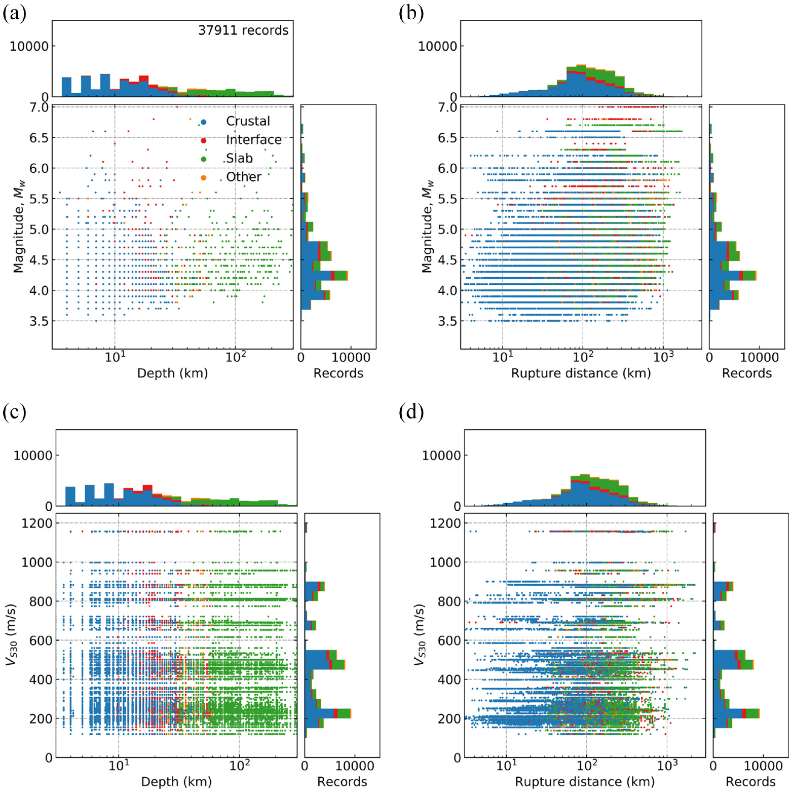
Figure 1 shows the tectonic mechanisms assigned to all records in the GeoNet catalog, and the distribution of records by magnitude, rupture distance, centroid depth, and time-averaged shear wave velocity in the top $30 m$ , $V_{S 30}$ . At shallow depths, the records are exclusively from crustal earthquakes, whereas, at large depths, the records are either from slab earthquakes or from other ambiguous origins. The seismogenic depths of the Hikurangi and Puysegur subduction interfaces are $10 - 47$ and $11 - 30 km$ , respectively (Hayes et al., 2018). Records are available for earthquakes from very shallow depths of less than a kilometer to very large depths up to $375 km$ ; however, most records are from earthquakes at depths less than $30 km$ .

Figure 1.

Metadata distributions for all ground-motion records in the GeoNet catalog: (a) magnitude and centroid depth; (b) magnitude and rupture distance; (c) $V_{S 30}$ and centroid depth; and (d) $V_{S 30}$ and rupture distance.

Figure 1 demonstrates that the catalog is primarily comprised of small-magnitude earthquakes with $4 < M_{w} < 5$ . There is a sharp reduction in the quantity of records from earthquakes with $M_{w} < 4$ and very few records from earthquakes larger than $M_{w} > 7$ . Rupture distances of $10 - 1000 km$ are well represented in the catalog. Most GeoNet stations are located on deep or soft soils (Kaiser et al., 2017); consequently, records were usually recorded on sites with $V_{S 30} < 760$ m/s; no records were recorded at sites with $V_{S 30} > 1200$ m/s.

Data processing and labeling

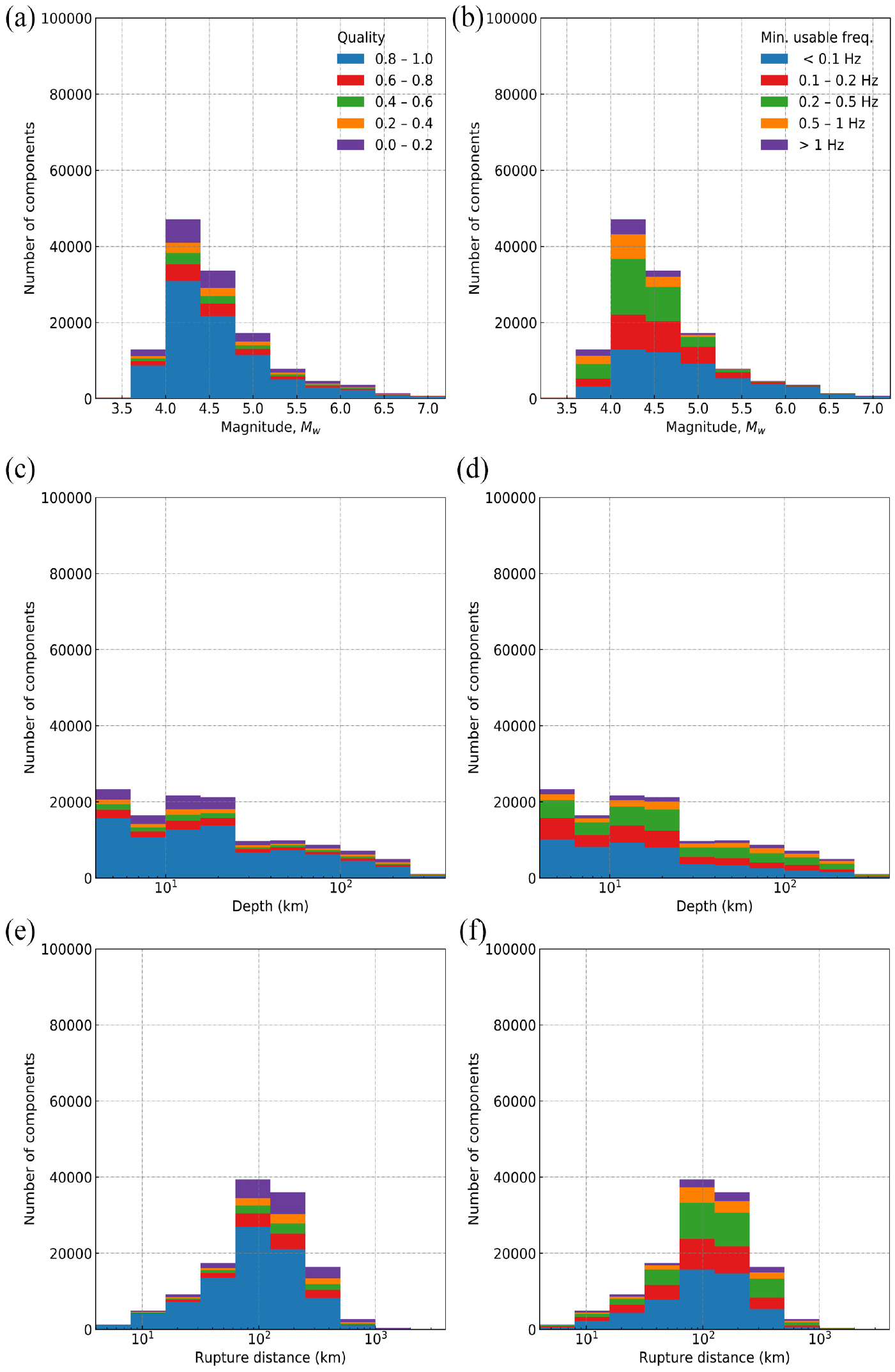
A data set of earthquake ground-motion records with varied magnitudes, rupture distances, centroid depths, and tectonic mechanisms was compiled for the development (training and validation) and testing of the developed deep-learning-based model. A record is defined herein to be the acceleration data for a given earthquake as recorded by a given instrument and is comprised of at least one, but typically three, orthogonal ground-motion components. Records for which the P-wave pick was poor—see Manual Assessment of Quality section—were not included in the development data set. Together, the development and testing data sets are comprised of 1096 three-component records which were manually labeled with a quality and minimum useable frequency on a component-by-component basis using the manual quality assessment framework discussed in the “Assessment framework” section. The labeling criteria that were used to assemble the component-level quality and minimum usable frequency labels are discussed in the “Manual assessment of quality” and “Manual assessment of minimum usable frequency” sections, respectively. 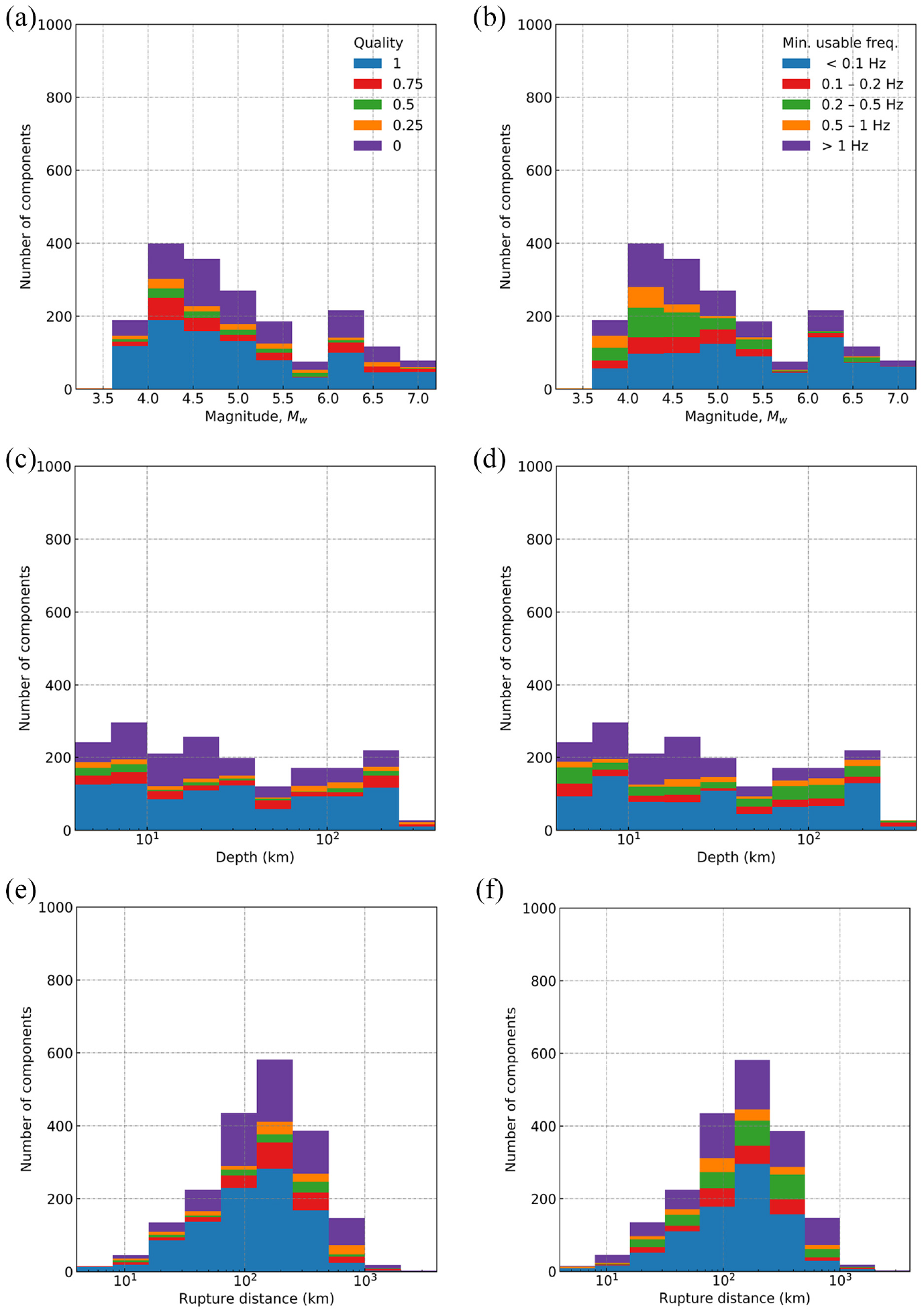The proportions and distributions of these manually assigned labels for various magnitudes, centroid depths, ruptures distances, and $V_{S 30}$ are shown in Figure 2 to provide context for the subsequent application of the deep-learning-based model to the GeoNet catalog.

Figure 2.

Manually labeled component quality and minimum usable frequency used for development and testing of the model (2070 components), sorted by: (a, b) magnitude; (c, d) centroid depth; and (e, f) rupture distance, respectively. Only components with complete site, source, and path metadata are shown. (a) Quality by magnitude, (b) minimum usable frequency by magnitude, (c) quality by depth, (d) minimum usable frequency by depth, (e) quality by distance, and (f) minimum usable frequency by distance.

Assessment framework

The quality of the multiple components which comprise a ground-motion record is not always uniform—occasionally, a record is comprised of two high-quality components and one low-quality component, or vice versa. Previously, the study by Bellagamba et al. (2019) assessed record quality on an overall record-by-record basis. This approach presents two main limitations: (1) effective training of the deep-learning-based model is reliant on well labeled training data and records with inter-component quality disparities labeled with a single quality label unnecessarily increases the dimensionality of the problem and reduces the precision of the labeled data and (2) there is no flexibility for the end user to enforce different minimum quality requirements for the three components.

Similar challenges were created by Bellagamba et al. (2019) due to the treatment of the minimum usable frequency—the frequency below which the noise content of a record overwhelms the desired ground-motion signal. In the study by Bellagamba et al. (2019), the minimum usable frequency was considered in the quality label determination and was implicitly included in the record quality label. While there are multiple other features that similarly affect the quality of a record which were also inherently included, such features are generally universal characteristics that affect record utility regardless of the application. This is not the case for the required minimum usable frequency, which, similar to whether the vertical component is required, can change depending on the application. In the approach of Bellagamba et al. (2019), there is no flexibility for the end user to adjust the required minimum usable frequency to reflect the unique demands of their intended engineering application.

To address these limitations, the manually labeled three-component ground-motion records were assessed in a component-by-component framework, with both a quality label and minimum usable frequency label provided for each component: that is, two labels per component, six labels per record. This treatment affords the end user with the flexibility to define their own explicit criteria to convert the component quality and minimum usable frequency estimations from the deep-learning-based model into a single record quality score, binary high-/low-quality determination (as explored in the “Effect of mapping on record estimations” section), or weights to be used in a logic tree. The general form of the quality mapping function is given in Equation 1 where $q_{x, y, z}$ are the component quality estimations and $f_{x, y, z}$ are the component minimum usable frequency estimations:

Q u a l i t y = f (q_{x}, q_{y}, q_{z}, f_{x}, f_{y}, f_{z})

(1)

Manual assessment of quality

Component quality was evaluated on a scale from 0 to 1, where 0 corresponds to low-quality and 1 corresponds to high-quality components. The transition from a label of 1 to 0 represents an overall degradation in component quality with consideration of multiple criteria which affect component quality. Three transitional quality labels of 0.25, 0.5, and 0.75 were used which correspond to marginally low-, marginal-, and marginally high-quality components, respectively; however, the delineations between these transitional labels are difficult to quantify in absolute terms. A detailed summary of the pre-processing applied and metrics considered to manually determine component quality is provided in Electronic Supplements B and C; only a high-level discussion of the main features considered is presented herein.

High-frequency noise exists in the acceleration-time series, sometimes as large amplitude accelerations visible prior to P-wave arrival. Where present in excess, that is, greater than about 10% of the peak ground acceleration (PGA), the quality label of the component was decreased to reflect deterioration in the component quality due to this high-frequency noise. If the acceleration amplitudes in the pre-event noise exceeded about 30% of the PGA, then the component was generally assessed to be low quality (i.e., labeled as 0).

Whether the entire seismic waveform is captured within the recorded duration can also affect the quality of the record, this was sometimes affected by late triggering or early termination. Late triggering (i.e., missed P-wave arrival) is severely detrimental to the utility of a record and easily identifiable; therefore, a binary approach to labeling these type of records was taken where components with late triggering were assigned to be low quality. As is typical for networks of modern and well-maintained strong ground-motion instruments (Patterson et al., 2007), instances of late triggering are rare in the GeoNet catalog.

A more frequently observed issue, particularly for earthquakes with large rupture distances, is when records terminate early in the coda. Although undesirable, the consequence of early termination on quality is continuous in nature: severely truncated components were labeled as low quality, while less egregious truncations were assigned marginal quality labels. In general, the coda waves were judged to be sufficiently diminished (i.e., high quality) if the amplitudes in the tail of the time series were about 15% or less of the PGA in the component, at above 40%, the component was generally assessed to be low quality.

The slope and shape of the Fourier amplitude spectrum (FAS) were also loosely considered in assessing component quality. In assembling a flatfile of KiK-net records, Dawood et al. (2016) required a smoothed low-frequency FAS slope of between 1 and 3. The rupture source model developed by Brune (1970) predicts a low-frequency FAS slope of 2. In this study, the corner frequencies of the component FAS were not computed; therefore, a strict assessment of the slope of the FAS was not possible; however, the slope of the FAS was loosely evaluated in the low-frequency range and slopes of approximately 2 were generally given a high-quality label.

Seismic instruments occasionally malfunction, and this can cause undesirable features in the record. Several common instrument malfunctions identified by Douglas (2003) were observed: for example, baseline offsets, gain discontinuity, low resolution, saturation, and spikes. It is possible that such components could be salvageable—depending on the intended engineering application, however, given the relative scarcity of such record components, and their compromised nature, this option was not pursued. Components with instrument malfunctions were labeled as low quality.

Ground-motion records may capture wavetrains from multiple earthquakes, and instances of multiple earthquakes in a single record were frequently observed in records from the GeoNet catalog. The important features of these records are the relative acceleration amplitudes and the degree of separation between the wavetrains. The practical implications of small amplitude well-separated foreshocks or aftershocks are negligible for almost all engineering applications, and Sabetta and Pugliese (1987) considered the first earthquake in a record containing multiple records as acceptable if the wavetrain did not overlap with subsequent P-wave arrivals in the time domain. On the other hand, the presence of multiple earthquakes of comparable amplitudes is detrimental to the utility of a record for most applications. The seismic wave arrival detector, PhaseNet (Zhu and Beroza, 2019), which was used in this study and implemented in feature extraction for the model, does not consider such distinctions; therefore, a pragmatic approach in which all components for records with multiple earthquakes were flagged as having multiple earthquakes and labeled as low quality. For some records PhaseNet produced inaccurate P- and S-wave arrival probability-time series; such records were kept in the testing data set to maintain impartiality, however, they were removed from the development data set to minimize confusion in the training data.

Manual assessment of minimum usable frequency

Strong ground-motion record components are, to varying degrees, contaminated by noise: instrument, environmental, societal, and even signal-generated, which limits their usable frequency range (Anthony et al., 2019; Boore and Bommer, 2005). These sources produce noise which affects different frequencies, and where noise is outside the frequency range of the earthquake ground motion, the affected frequencies can be filtered out prior to using the record in engineering applications. However, if noise overlaps with the earthquake ground-motion frequencies, then it may not be possible. The best practice is to establish a frequency range in which the records can be used and to convey this information with the ground-motion data (Boore and Bommer, 2005).

In general, the GeoNet catalog contains records that were recorded on modern, high-performance, digital accelerometers with high natural frequencies and sampling rates (Patterson et al., 2007); therefore, significant high-frequency noise was not common. However, where encountered, such high-frequency noise generally pervaded the frequency range of engineering interest $(0.01 - 10 Hz)$ to an extent that made determining a maximum usable frequency impractical. High-frequency noise was therefore considered a criterion in determining the component quality label (see the “Manual assessment of quality” section).

The minimum usable frequency, $f_{\min}$ , is a more nuanced consideration that is affected by low-frequency noise—often instrumental—and the signal strength at low frequencies. In order to advise on the minimum usable frequency of a component, each component was assigned a minimum usable frequency label from 0.01 to 10 Hz. This minimum usable frequency was determined based on the spectral signal-to-noise ratio (SNR) of the smoothed FAS of the signal portion (time series after P-wave arrival, containing earthquake signal and also noise) to the smoothed FAS of the noise portion (time series prior to P-wave arrival, containing only noise). Smoothing was done with Konno-Ohmachi matrices with a smoothing bandwidth of $b = 40$ (Beyreuther et al., 2010; Konno and Ohmachi, 1998). A minimum SNR 3 is often used as an acceptance criterion (Boore and Bommer, 2005); however, records with relatively small magnitudes and large rupture distances are being considered; therefore, a more lenient threshold of SNR 2 was used. If a $SNR > 2$ was not sustained in the frequency domain, then the minimum usable frequency was labeled as $f_{\min} = 10 Hz$ ; this scenario almost always coincides with a low-quality label, in which case the minimum usable frequency label is moot. A detailed summary of the metrics considered to determine the manual minimum usable frequency labels is provided in Electronic Supplement D.

Neural network design and development

High-quality ground-motion records are systematically different than low-quality records, and with appropriate features that capture these differences, it is possible to estimate the quality of a given record. As manual quality assessment is non-trivial and time intensive, a machine learning approach is well suited to this problem. This section summarizes major aspects of the deep-learning-based ground-motion classifier model, including feature identification and extraction, model architecture, and development. Full details are provided in Electronic Supplements F to H.

Feature identification and extraction

For general quality estimation of a record, a set of 18 scalar features was used. Two special cases in quality estimation were considered, records with multiple earthquakes and malfunctioned records, for which an additional six and five features were introduced, respectively. This set of 29 features was complemented by an SNR series comprised of 100 values computed at evenly distributed (in log space) frequencies from 0.01 to 25 Hz, allowing estimation of the minimum usable frequency and enhanced quality estimation.

P-wave arrival times were needed to divide the acceleration-time series (in the time domain) into a noise portion (prior to P-wave arrival) and a signal portion (after P-wave arrival) for the computation of the SNR series and many of the scalar features. The deep-learning arrival time picker, PhaseNet (Zhu and Beroza, 2019), was used as it was observed to outperform other phase-pickers which use short-term versus long-term averages, such as those based on work by Akazawa (2004) or Baer and Kradolfer (1987). An additional useful characteristic of PhaseNet is that it outputs probability-time series for both P- and S-wave arrivals, which can be used for the detection of multiple earthquakes.

The reliance of the input features on separation into noise and signal portion means that some records cannot be processed due to limitations such as insufficient pre-event noise, incorrect P-wave pick, and others. In such cases, the feature extraction for the record fails and classification is not possible. For the full set of requirements that a record must meet, see Electronic Supplement F.

The 18 general quality estimation features are mostly based on the ground-motion classifier by Bellagamba et al. (2019), which measure high-frequency noise, early termination, late triggering, FAS shape, and SNR over various frequency bands. As estimation is done per component, this includes an additional feature that indicates the component orientation (horizontal or vertical).

Instrument malfunction features were computed based on the third and fourth derivatives of position: jerk and snap (Thompson, 2011) and were generally designed to detect odd acceleration-time series characteristics including baseline offsets, gain discontinuity, low-resolution, saturation or flatline, and spikes.

Multiple earthquake features were computed from both the P- and S-wave arrival probability-time series produced by PhaseNet. These multiple earthquake features were based on comparing the widths and amplitudes of secondary probability peaks to those associated with the arrival of the primary wavetrain. As PhaseNet operates on three-component records, these features are identical across a given record, unlike the other input features which are computed per component.

All scalar features, except the “is vertical” flag, were converted into dimensionless form via mean and standard deviation (Raschka et al., 2022).

Architecture

The model has two sub-models (see Figure 3) which correspond to the two different input types: the scalar input features and the SNR series. The scalar sub-model consists of 2 fully connected layers, each with 32 units.

Figure 3.

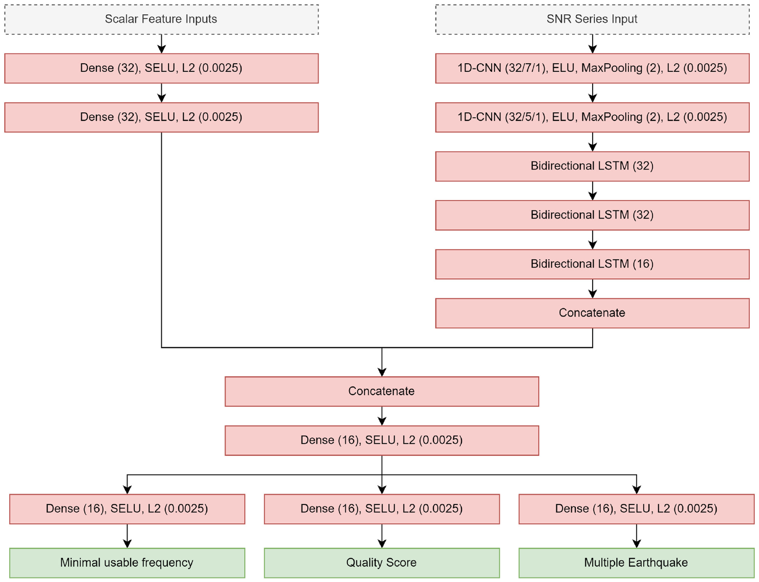
Model architecture: scalar input neural network (top left); SNR series neural network (top right); and concatenation and fully connected neural network with output layers.

Feature extraction of the SNR series was done using a set of two 1D convolution layers with L2 regularization (Raschka et al., 2022), each followed by a max-pooling layer with a pooling size of 2. The extracted feature series are then passed through 3 layers of bi-directional LSTM (Hochreiter and Schmidhuber, 1997) cells to produce a context vector of size 64.

The output of both of these sub-models is then concatenated and passed through a fully connected layer, followed by an additional fully connected layer per output. All fully connected hidden layers used the SELU activation function (Clevert et al., 2016; Klambauer et al., 2017), L2 regularization (Biewald, 2020), and were initialized using the “LeCunNormal” approach (LeCun et al., 2012). For the full model hyperparameters, refer to Electronic Supplement H.

The model outputs the quality score, ranging from 0.0 (worst) to 1.0 (best), the minimum usable frequency (0.01–10.0), and a multiple earthquake flag (True or False).

Model training

The model was trained via back-propagation using the Adam optimizer (Kingma and Ba, 2017) with a batch size of 32 samples (components) and an initial learning rate of $1 e - 3$ , which was reduced by a factor of 0.5 on plateaus (based on the validation loss). In addition, early stopping and storing of the best model weights (based on validation loss) were used during training to prevent over-fitting (and reduce training time), with the best model weights restored at the end of training. The loss functions used for each of the outputs were the Huber loss (Huber, 1964) for the quality score and the minimum usable frequency and the binary cross-entropy for the multiple earthquake flag. To account for the fact that the minimum usable frequency has no meaning for low-quality records, it was weighted such that the loss goes to 0 as the “true” manually labeled component quality goes to 0. The combined loss is then computed as a weighted sum, with the weights chosen manually to account for the difference in scale and importance of the outputs. For full details on the loss function used, see Electronic Supplement H.

Results

In this section, the accuracy of the component-level estimations from the model is assessed using the independent test data set, then the distribution of component-level estimations for the entire GeoNet catalog is discussed. The effect of mapping on rates of high-quality record-level quality determinations within GeoNet is first explored, and then observations from this exploration are used to inform an attempt to reproduce the quality labels of three quality-labeled data sets from other studies.

Component estimation performance

To evaluate the performance of component quality and minimum usable frequency estimations from the model, a testing data set of 540 manually labeled components was used (180 three-component records). This labeled data was not used for training or validation of the model, nor was it curated to remove poor PhaseNet results; therefore, it represents an unbiased test of the model performance. Performance was assessed using a residual analysis framework, where the component quality and minimum usable frequency estimation residuals were computed using Equations 2 and 3, respectively:

Δ q = q^{t r u e} - q^{e s t i m a t e d}

(2)

Δ f = \ln ({f_{\min}}^{true}) - \ln ({f_{\min}}^{estimated})

(3)

The bias of $Δ q$ was close to 0 for all tectonic mechanisms in the testing data set, and the bias of $Δ f$ (determined only for components with $q^{true} \geq 0.75$ ) indicates that the minimum usable frequency was consistently over-estimated (i.e., ${f_{\min}}^{true}$ is lower). The bias of $Δ q$ is smaller than that of $Δ f$ which reflects the increased importance (i.e., optimization weight) placed on quality estimations during model development (see the “Model training” section). Neither set of residuals correlate strongly with metadata properties of the records such as magnitude, centroid depth, or rupture distance, as shown in Figure 4.

Figure 4.

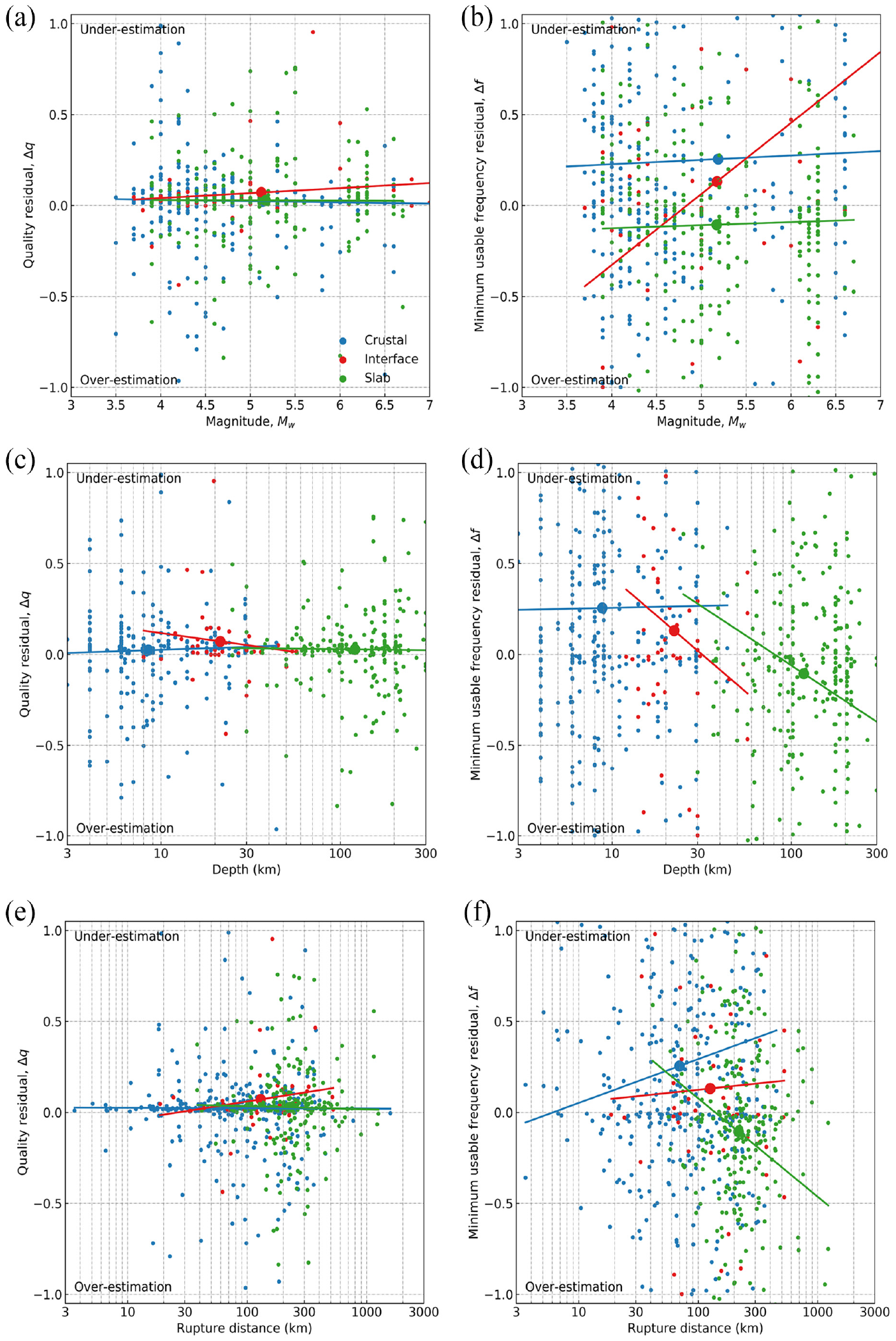
Estimated component quality and minimum usable frequency residuals for labeled crustal, interface, and slab ground-motion records in the test data set: (a, b) magnitude; (c, d) centroid depth; and (e, f) rupture distance, respectively. The mean residual is shown as the large circle marker, and linear regression line of best fit is shown for each tectonic type within each panel. (a) Quality residual by magnitude, (b) minimum usable frequency residual by magnitude, (c) quality residual by depth, (d) minimum usable frequency residual by depth, (e) quality residual by distance, and (f) minimum usable frequency residual by distance.

Component estimations for GeoNet

When applied to the complete GeoNet catalog, quality and minimum usable frequency estimations were obtained for all components (Figure 5). As shown in Figure 5a, c, and e, 65% of components are estimated to have quality greater than 0.8 and only 13% of records components are assigned low-quality scores below 0.2; this indicates that the catalog is comprised of predominantly high-quality record components. Similarly, as shown in Figure 5b, d, and f, the majority of components are observed to have relatively low minimum usable frequencies: 35% of components are estimated to have minimum usable frequencies below $0.1 Hz$ and only 7% of records components are assigned minimum usable frequencies above $1 Hz$ .

Figure 5.

Estimated component quality and minimum usable frequency for all ground motions (130,194 components) in the GeoNet catalog by: (a, b) magnitude; (c, d) centroid depth; and (e, f) rupture distance, respectively. Only components with complete site, source, and path metadata are shown. (a) Quality by magnitude, (b) minimum usable frequency by magnitude, (c) quality by depth, (d) minimum usable frequency by depth, (e) quality by distance, and (f) minimum usable frequency by distance.

The component estimations were uncorrelated with site properties such as $V_{S 30}$ and most earthquake source characteristics including tectonic mechanism and centroid depth when controlled for constant rupture distance. As was expected, the proportion of record components with high qualities and low minimum usable frequencies decreases with increasing rupture distance due to increased attenuation of seismic waveforms to small amplitudes which are less prominent among background noise.

For a given rupture distance, the proportion of high-quality components is greater for larger magnitude earthquakes; however, because such large magnitude earthquakes are able to be recorded at greater rupture distances, this effect is diminished when considering all record components for a given magnitude, as presented in Figure 5. However, the minimum usable frequency has significant dependence on magnitude even without controlling for rupture distance; at large magnitudes, the proportion of components with very low minimum usable frequencies is relatively large; this is suspected to be the result of corner-frequency scaling with magnitude.

Effect of mapping on record estimations

There are many possible ways in which the component-level quality and minimum usable frequency estimations from the model can be implemented by engineers and seismologists. One possible application is converting the component-level estimations into a binary record-level quality determination. In this section, the effects of various possible approaches are explored considering all records in the GeoNet catalog (see “GeoNet catalog of records” section), which also aids in the subsequent comparison of the model predictions against prior data sets that have been compiled.

In engineering and seismological applications, the most common combinations of components used are as follows: (1) two orthogonal horizontal components only and (2) all three orthogonal components, and hence these are the combinations that will be considered. Mapping functions are used in this approach to combine the two or three component-level estimations into a single quality and minimum usable frequency value for each record. In this examination of the effect of mapping, the mapped record-level quality and minimum usable frequency estimations were then considered against a range of possible acceptance thresholds; that is, combined acceptance thresholds which considered quality and minimum usable frequency estimations simultaneously were not considered.

Five possible component mapping functions were considered (Figure 6), in order of smallest to largest resultant, these are as follows: (1) minimum (appropriate for quality only), (2) harmonic mean, (3) geometric mean, (4) arithmetic mean, and (5) maximum (appropriate for frequency only). The minimum is not appropriate for mapping the minimum usable frequency estimations because it is not realistic to assess a record based on the best-performing component only; similarly, the maximum is not appropriate for mapping the quality estimations. Of these mapping functions, either the minimum or arithmetic mean is most appropriate for quality, and the maximum or geometric mean is most appropriate for minimum usable frequency. All three types of means are included as generic functional examples to illustrate the sensitivity of the binary quality determination to the mapping function form.

Figure 6.

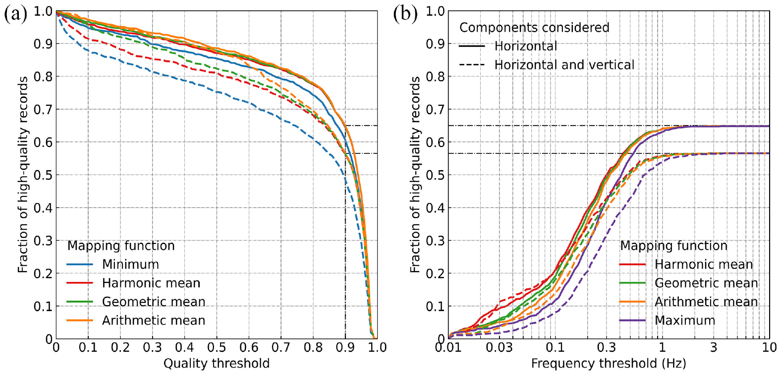
Fraction of records in the GeoNet catalog which are determined to be high-quality using different mappings of component-level (a) quality and (b) minimum usable frequency estimations and acceptance thresholds: (a) effect of quality mapping and acceptance threshold with no minimum usable frequency acceptance threshold enforced and (b) effect of minimum usable frequency mapping and acceptance threshold with a quality threshold of 0.9 enforced on the arithmetic mean of the component quality estimations.

The tendency of the mapping function to produce either small or large record-level values influences the fraction of records determined to be high quality. Mapping functions that produce larger values are less stringent for assessing record quality, and the opposite is true for minimum usable frequency. This is because mapped quality is compared against an acceptance threshold which must be exceeded in order for the record to be determined to be high quality while the mapped minimum usable frequency is compared against an acceptance threshold which it must be below.

As shown in Figure 6a, the majority of records have component qualities above 0.9; below this threshold, the decline in high-quality records is approximately linear for all mapping functions. Which mapping function is used has little effect on two-component records and only a minor effect on records with a vertical component. Using the minimum as opposed to the arithmetic mean results in approximately 10–20% fewer high-quality records for quality thresholds between 0.1 and 0.9.

Figure 6b shows the effect of the functional form of the component minimum usable frequency mapping for records satisfying a quality threshold of 0.9 based on the arithmetic mean of the component estimations—the minimum usable frequency is moot for low-quality records. The general effect of minimum usable frequency mapping is similar regardless of this quality threshold, but the asymptote at high-frequency thresholds differs depending on the fraction of records that meet the specified quality threshold (i.e., 0.9 for this example). In the limit case of a quality threshold of 0, the asymptote would occur at 1. Figure 6b illustrates that there are few records that satisfy minimum usable frequency requirements below $0.1 Hz$ ; most records fall between 0.1 and 1 Hz. The fraction of accepted records begins its plateau at approximately $1 Hz$ indicating that very few estimated component minimum usable frequencies are between 1 and 10 Hz. Additional plots illustrating the effect of mapping forms on the fraction of high-quality records in the GeoNet catalog are provided in Electronic Supplement J.

Performance on quality-labeled data sets

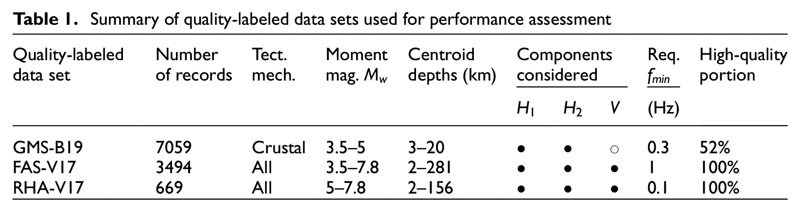
To assess the performance of the model at classifying records for various engineering applications, three quality-labeled data sets compiled from other studies (Table 1) were considered. The metadata distributions for records in these data sets are shown in Figure 7. These data sets were comprised of records with binary high-/low-quality labels which were manually determined based on various component quality and minimum usable frequency criteria.

Table 1.

Summary of quality-labeled data sets used for performance assessment

Quality-labeled data set	Number of records	Tect. mech.	Moment mag. $M_{w}$	Centroid depths (km)	Components considered			Req. $f_{\min}$	High-quality portion
					$H_{1}$	$H_{2}$	$V$	(Hz)	High-quality portion
GMS-B19	7059	Crustal	3.5–5	3–20	•	•	○	0.3	52%
FAS-V17	3494	All	3.5–7.8	2–281	•	•	•	1	100%
RHA-V17	669	All	5–7.8	2–156	•	•	•	0.1	100%

Figure 7.

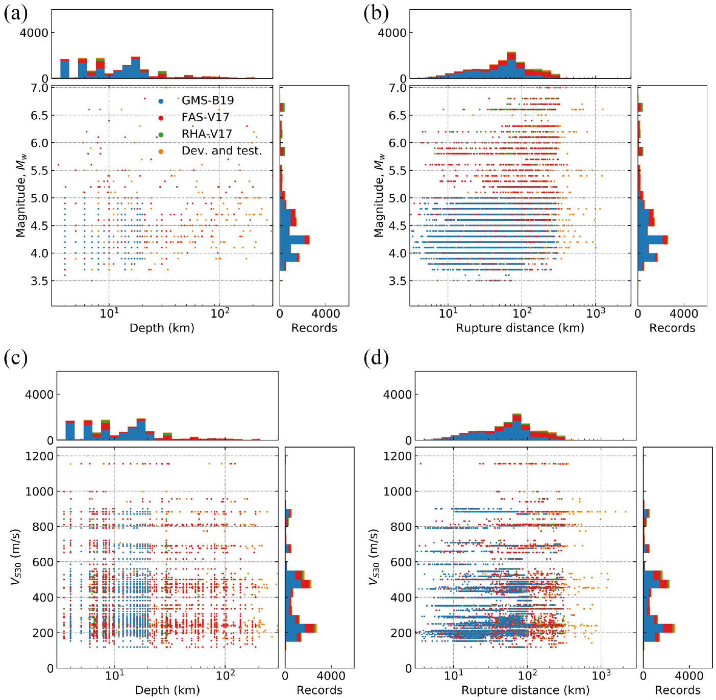
Metadata distributions for ground-motion records in the quality-labeled data sets and those manually labeled on a component-by-component basis for the development and testing of the model: (a) magnitude and centroid depth; (b) magnitude and rupture distance; (c) $V_{S 30}$ and centroid depth; and (d) $V_{S 30}$ and rupture distance.

The first data set, GMS-B19, contains 7059 high- and low-quality small-magnitude crustal records labeled based on their suitability for ground-motion simulation validation. The quality determination of these records was made for validation of physics-based ground-motion simulation toward its use in probabilistic seismic hazard analysis (Bellagamba et al., 2019); therefore, only the quality of the horizontal components was considered and an approximate minimum usable frequency of $0.3 Hz$ was enforced for each horizontal component as a requisite for a high-quality record label.

The second data set, FAS-V17, contains only high-quality records from all sources screened to produce the three-component FAS database from Van Houtte et al. (2017). Records included in FAS-V17 were required to have a minimum usable frequency of $1 Hz$ or lower from all three components.

The third data set, RHA-V17, contains only high-quality records from all sources recommended for use by engineers in three-dimensional response history analysis of structures (Van Houtte et al., 2017), which is a subset of the records in FAS-V17. Records included in this data set were required to have three high-quality components each with a minimum usable frequency of $0.1 Hz$ or lower.

For performance assessment of the deep-learning model on these quality-labeled data sets, the component estimations (six per record) from the model needed to be mapped into a single binary high/low-quality decision to match the form of the quality labels in the quality-labeled data sets. As discussed in the “Effect of mapping on record estimations” section, the choice of the mapping function is non-trivial and can have a significant effect on the binary high-/low-quality record-level estimations. For the performance comparison in this section, an approach thought to be similar to that which might be taken by an engineer or seismologist was adopted.

For each data set, only the quality and minimum usable frequency estimations for the relevant components were considered, i.e., the vertical components in GMS-B19 were ignored. For all data sets, the arithmetic mean of the quality estimations of the considered components was compared against an acceptance threshold of 0.5. The binary high-/low-quality estimations for the records were not sensitive to the selection of this threshold, because most of the estimated component qualities are close to either 0 or 1 (Figure 5a, c, and e). The geometric mean of the minimum usable frequency estimations was compared against the minimum usable frequency criteria specific to each data set (Table 1). It was found that comparing means of the component-level estimations has the desirable effect of averaging out component-level estimation residuals for a given ground-motion record (the component residuals for a given record are only partially correlated).

As performance benchmarks, two neural networks developed for small-magnitude crustal earthquake records by Bellagamba et al. (2019) were also considered: (1) Canterbury neural network and (2) Canterbury-Wellington neural network. The Canterbury-Wellington neural network, which was developed using a more geographically diverse set of records, was found to perform better than the Canterbury neural network for all three data sets; therefore, only the estimations of the Canterbury-Wellington neural network are presented herein. The assessment criteria of the Bellagamba et al. (2019) models are not strictly aligned with the labeling of FAS-V17 and RHA-V17 data sets. However, the Canterbury-Wellington model is still used as a benchmark since guidance for its use in applications outside of ground-motion simulation validation is not provided in that study. Inferences related to this misalignment are expanded upon in the following interpretation of results.

Various performance metrics were considered to evaluate the performance of the Canterbury-Wellington neural network and the deep-learning model in this study on the binary record-level estimations in the three quality-labeled data sets and mapped testing data set. These included recall, precision, specificity, accuracy, $F_{1}$ score, and weighted Youden index $(J_{w})$ (Li et al., 2013; Youden, 1950), the formulations for which are given in Electronic Supplement I. These are all measures of classification correctness and are based on comparing numbers of true positives $(TP)$ , true negatives $(TN)$ , false positives $(FP)$ , and false negatives $(FN)$ in a labeled data set, where $w$ is the ratio of all $TP$ and $FN$ to the total number of records. For the FAS-V17 and RHA-V17 data sets, which contain only high-quality records, only the accuracy, recall, $F_{1}$ score, and weighted Youden index provided meaningful measures of performance. The accuracy, taken as the percentage of correct estimations, was found to be a simple yet effective metric for comparison across the data set domains and is considered in more detail across the domain of magnitudes and rupture distances in Figure 8.

Figure 8.

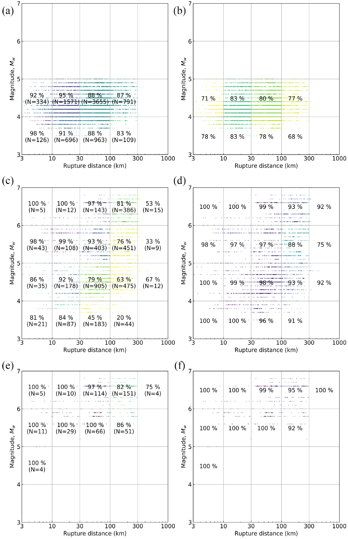
Estimation accuracy (% correct), by magnitude-rupture distance bins, of the Canterbury-Wellington neural network (CW) and the model in this study on the three quality-labeled data sets: GMS-B19; FAS-V17; and RHA-V17. Records are colored by the average estimation accuracy in each bin, and N is the number of records. (a) CW on GMS-B19, (b) the model on GMS-B19, (c) CW on FAS-V17, (d) the model on FAS-V17, (e) CW on RHA-V17, and (f) the model on RHA-V17.

The Canterbury-Wellington neural network was developed using the quality-labeled records in the GMS-B19 data set as training data; therefore, although its selection criteria are properly aligned with the quality-labeled records in this data set, it has an artificial advantage because it was trained on this data, whereas the model was not. As shown in Figure 8, the Canterbury-Wellington neural network performed very well on this data set for all rupture distances and magnitudes.

For FAS-V17, the minimum usable frequency requirements $(1.0 Hz)$ are not compatible with the assessment criteria for the Canterbury-Wellington neural network, which required the minimum usable frequency to be lower than roughly $0.3 Hz$ . Therefore, the Canterbury-Wellington neural network applies too stringent a requirement on the minimum usable frequency and estimates many of the ground-motion records to be low quality despite being manually labeled as high quality. In other words, a record with a minimum usable frequency between approximately 0.3 and 1.0 Hz would likely be considered low quality by the Canterbury-Wellington model but is labeled as high quality within the FAS-V17 assessment criteria.

For RHA-V17, which contains records usable to $0.1 Hz$ , the Canterbury-Wellington neural network is too lenient in its assessment of the minimum usable frequency. The Canterbury-Wellington neural network appears to perform well on this data set, but this apparent performance is inflated because all ground motions are high quality and likely on the very high-quality end of the spectrum. Therefore, the results shown only indicate the accuracy in predicting very high-quality records. It does not provide any indication of the accuracy in predicting low-quality records. Although the performance here is generally good, the accuracy of the estimations can be seen to decrease for records in this data set from large magnitude or large rupture distance earthquakes (Figure 8e)—i.e., conditions for which it was not developed.

The implicit quality criteria upon which the Canterbury-Wellington neural network was developed (i.e., that of GMS-B19 in Table 1) do not align with the selection criteria of the FAS-V17 and RHA-V17 data sets. This highlights the advantage of the model developed in this study’s flexible mapping approach based on component-level quality and minimum usable frequency estimations.

From Table 2, it can be seen that the model in this study performs significantly better than the Canterbury-Wellington neural network of Bellagamba et al. (2019) on these two data sets for all metrics considered. From Figure 8b, d, and f, it can be seen that the mapped record-level estimation accuracy of the model is high for all magnitudes and rupture distances in all three data sets. Performance is the best for large magnitudes and small rupture distances and generally degrades for smaller magnitudes and larger rupture distances which are conditions that are likely to produce records of marginal quality and for which earthquake ground-motion records are of less utility in most engineering applications.

Table 2.

Estimation performance, as quantified with various metrics, of the Canterbury-Wellington neural network (CW) by Bellagamba et al. (2019), and the model in this study (M) on the testing data set and three quality-labeled data sets. All metrics range between 0 and 1, where 1 indicates perfect performance

Data set	Recall		Precision		Specificity		Accuracy		$F_{1}$ score		$J_{w}$
Data set	CW	M	CW	M	CW	M	CW	M	CW	M	CW	M
Testing data	0.58	0.83	0.98	0.96	0.94	0.84	0.64	0.83	0.72	0.89	0.28	0.66
GMS-B19	0.85	0.94	0.95	0.75	0.95	0.62	0.9	0.8	0.9	0.83	0.79	0.59
FAS-V17	0.84	0.95	—	—	—	—	0.84	0.95	0.91	0.97	0.68	0.9
RHA-V17	0.88	0.95	—	—	—	—	0.88	0.95	0.94	0.97	0.77	0.9

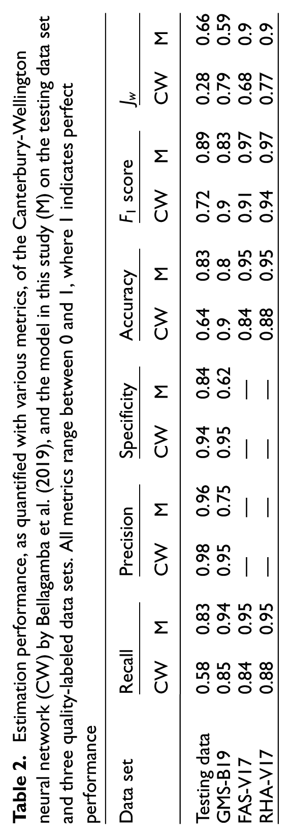
The performance of the model, as quantified by the metrics in Table 2, is high for all data sets. Relative variations of recall, precision, and specificity would occur for different approaches to binary record-level mapping, of which there are many; therefore, too much emphasis should not be placed on any one of these metrics. Similarly, although the binary record-level mapping was intended to mimic the logic applied by the authors of each of the three quality-labeled data sets, some mismatch is inevitable and so it is expected that there would be estimation errors.

For an additional comparison of independent data, the testing data set was considered with mapping to record-level estimations, and the performance of this data set is given in Table 2. The criteria (i.e., quality and frequency thresholds and components considered) for labeling the quality of records in GMS-B19, for which the Canterbury-Wellington neural network was calibrated, were applied to the component-level labels in the testing data set (the component-level estimations from the model were also mapped using the same logic). This mapped quality-labeled data is consistent with the selection criteria of both the Canterbury-Wellington neural network and the model, and was not used in the development of either; therefore, this comparison gives the best indication of the relative performance between the two. The model performs better than the Canterbury-Wellington neural network on the independent testing data set for earthquakes of all magnitudes, tectonic mechanisms, and rupture distances as indicated by the metrics which measure the overall performance (accuracy, $F_{1}$ score, and weighted Youden index), although the precision and specificity are slightly worse.

Conclusion

A deep-learning-based model was developed to provide an automated method of ground-motion record quality assessment which can determine the quality of a ground-motion record for a wide range of engineering applications. The model provides accurate quality and minimum usable frequency estimations on a component-by-component basis for ground-motion records from small- and moderate-magnitude earthquakes of all tectonic classifications for various rupture distances and site conditions; although it was developed with NZ ground motions, it is expected to extend well to other regions. Furthermore, it can effectively identify record components with instrument malfunction or multiple earthquake wavetrains and interprets such components as low quality.

If desired, mapping of component-level estimations to a record-level quality determination can be tailored to satisfy the demands of specific applications, such as whether a vertical component is required and what minimum usable frequency is needed. Adjustment of quality and minimum usable frequency thresholds, and the manner in which they are applied, allows for varying degrees and dimensions of selectivity to be enforced. Alternatively, the component estimations can be used for other purposes such as to establish weights in an analysis logic tree or to evaluate the performance of various recording stations and inform maintenance activities. The inherent flexibility of the model makes it applicable to a range of engineering applications and the manner in which the component-level estimations may be used is left as flexible as possible to encourage its use by engineers and seismologists at their discretion.

In the future, the model is expected to be used for classifying new ground-motion records as they are added to GeoNet and other global catalogs; these are expected to increase in number as more stations (including low-cost alternatives) are installed. The model is well suited to this demand; however, it has several limitations. Because the model relies significantly on PhaseNet, its performance is bounded by PhaseNet and the model performs poorly where PhaseNet performs poorly. The model is only applicable for three-component records, or for one-component records where the component is in the vertical direction. The feature computation takes significant computational time and is limited to records that satisfy requirements of duration, timestep, and P-wave arrival. The data set used for the model development is relatively small and contains few records for large magnitudes and short rupture distances; future studies could implement data augmentation techniques or consider global catalogs to expand the data set. Components of each record were handled independently in the model; however, future studies could consider the correlation of components within each record. As the capability of machine learning continues to improve, other deep-learning architectures, such as one that uses the entire acceleration-time series as input rather than extracted features, could be implemented and may be able to further improve performance.

Resources

The implementation of this quality classification tool has been done in Python 3.6 using the following main libraries ObsPy (Krischer et al., 2015) to process ground motions and PhaseNet (Zhu and Beroza, 2019) for P- and S-wave arrival and multiple earthquake detection. Keras (Chollet et al., 2018) and TensorFlow (Abadi et al., 2016) were used to create and train the model, along with NumPy (Harris et al., 2020), SciPy, and Pandas (Virtanen et al., 2020) for general scientific computing. Matplotlib (Hunter, 2007) and scikit-learn (Pedregosa et al., 2011) were used for plotting and general machine learning functionality, respectively. Ground-motion records were obtained from the GeoNet file transfer protocol (GeoNet, 2020). The model is available as a GitHub repository: https://github.com/ucgmsim/gm classifier.

Supplemental Material

sj-pdf-1-eqs-10.1177_87552930231195113 – Supplemental material for A deep-learning-based model for quality assessment of earthquake-induced ground-motion records

Supplemental material, sj-pdf-1-eqs-10.1177_87552930231195113 for A deep-learning-based model for quality assessment of earthquake-induced ground-motion records by Michael Dupuis, Claudio Schill, Robin Lee and Brendon Bradley in Earthquake Spectra

Footnotes

Declaration of conflicting interests

The author(s) declared no potential conflicts of interest with respect to the research, authorship, and/or publication of this article.

Funding

The author(s) disclosed receipt of the following financial support for the research, authorship, and/or publication of this article: This project was (partially) supported by Te Hiranga Rū QuakeCoRE, an Aotearoa New Zealand Tertiary Education Commission-funded Centre. This is QuakeCoRE publication number 890. Support was also provided through the Commonwealth Scholarship and Fellowship Plan funded by the Government of Canada, and the Royal Society of New Zealand’s Rutherford Postdoctoral Fellowship and Marsden Fund.

ORCID iDs

Michael Dupuis

Robin Lee

Brendon Bradley

Supplemental material

Supplemental material for this article is available online.

References

Abadi

Barham

Chen

Davis

Dean

Devin

Ghemawat

Irving

Isard

Kudlur

Levenberg

Monga

Moore

Murray

Steiner

Tucker

Vasudevan

Warden

Wicke

Zheng

(2016) Tensorflow: A system for large-scale machine learning. In: 12th USENIX symposium on operating systems design and implementation (OSDI 16), Savannah, GA, 2–4 November, pp. 265–283. Berkeley, CA: USENIX.

Akazawa

(2004) A technique for automatic detection of onset time of p-and s-phases in strong motion records. In: Proceedings of the 13th World Conf. on Earthquake Engineering, Vancouver, BC, Canada, 1–6 August.

Ancheta

Darragh

Stewart

Seyhan

Silva

Chiou

BSJ

Wooddell

Graves

Kottke

Boore

Kishida

Donahue

(2014) NGA-west2 database. Earthquake Spectra 30(3): 989–1005.

Anthony

Ringler

Wilson

Wolin

(2019) Do low-cost seismographs perform well enough for your network? An overview of laboratory tests and field observations of the OSOP raspberry shake 4D. Seismological Research Letters 90(1): 219–228.

Atkinson

Boore

(2003) Empirical ground-motion relations for subduction-zone earthquakes and their application to Cascadia and other regions. Bulletin of the Seismological Society of America 93(4): 1703–1729.

Baer

Kradolfer

(1987) An automatic phase picker for local and teleseismic events. Bulletin of the Seismological Society of America 77(4): 1437–1445.

Bellagamba

Lee

Bradley

(2019) A neural network for automated quality screening of ground motion records from small magnitude earthquakes. Earthquake Spectra 35(4): 1637–1661.

Beyreuther

Barsch

Krischer

Megies

Behr

Wassermann

(2010) Obspy: A python toolbox for seismology. Seismological Research Letters 81(3): 530–533.

Biewald

(2020) Experiment tracking with weights and biases. Available at: https://www.wandb.com/

10.

Bijelić

Lin

Deierlein

(2018) Validation of the SCEC broadband platform simulations for tall building risk assessments considering spectral shape and duration of the ground motion. Earthquake Engineering & Structural Dynamics 47(11): 2233–2251.

11.

Boore

Bommer

(2005) Processing of strong-motion accelerograms: Needs, options and consequences. Soil Dynamics and Earthquake Engineering 25(2): 93–115.

12.

Bozorgnia

Stewart

Abrahamson

(2020) Data resources for NGA-subduction project. PEER no. Report 2020/2, March 16. Berkeley, CA:Pacific Earthquake Engineering Research Center.

13.

Brune

(1970) Tectonic stress and the spectra of seismic shear waves from earthquakes. Journal of Geophysical Research 75(26): 4997–5009.

14.

Burks

Baker

(2014) Validation of ground-motion simulations through simple proxies for the response of engineered systems. Bulletin of the Seismological Society of America 104(4): 1930–1946.

15.

Cauzzi

Clinton

(2013) A high-and low-noise model for high-quality strong-motion accelerometer stations. Earthquake Spectra 29(1): 85–102.

16.

Chiou

Darragh

Gregor

Silva

(2008) NGA project strong-motion database. Earthquake Spectra 24(1): 23–44.

17.

Chollet

and others (2018) Keras: The python deep learning library. Astrophysics Source Code Library 2018: ascl–1806.

18.

Clevert

Unterthiner

Hochreiter

(2016) Fast and accurate deep network learning by exponential linear units (ELUs). arXiv:1511.07289.

19.

Dawood

Rodriguez-Marek

Bayless

Goulet

Thompson

(2016) A flatfile for the kik-net database processed using an automated protocol. Earthquake Spectra 32(2): 1281–1302.

20.

Douglas

(2003) What is a poor quality strong-motion record? Bulletin of Earthquake Engineering 1(1): 141–156.

21.

Evans

Allen

Chung

Cochran

Guy

Hellweg

Lawrence

(2014) Performance of several low-cost accelerometers. Seismological Research Letters 85(1): 147–158.

22.

GeoNet (2020) Index of strong/processed/raw. Available at: https://www.geonet.org.nz/data/access/FDSN

23.

Géron

(2019) Hands-On Machine Learning with Scikit-learn, Keras, and Tensorflow: Concepts, Tools, and Techniques to Build Intelligent Systems. Sebastopol, CA: O’Reilly Media.

24.

Goulet

Abrahamson

Somerville

Wooddell

(2015) The SCEC broadband platform validation exercise: Methodology for code validation in the context of seismic-hazard analyses. Seismological Research Letters 86(1): 17–26.

25.

Harris

Millman

Van der Walt

Gommers

Virtanen

Cournapeau

Wieser

Taylor

Berg

Smith

Kern

Picus

Hoyer

van Kerkwijk

Brett

Haldane

del Río

Wiebe

Peterson

Gérard-Marchant

Sheppard

Reddy

Weckesser

Abbasi

Gohlke

Oliphant

(2020) Array programming with NumPy. Nature 585(7825): 357–362.

26.

Hartzell

(1978) Earthquake aftershocks as green’s functions. Geophysical Research Letters 5(1): 1–4.

27.

Hassani

Atkinson

(2016) Applicability of the NGA-west2 site-effects model for Central and Eastern North America. Bulletin of the Seismological Society of America 106(3): 1331–1341.

28.

Hayes

Moore

Portner

Hearne

Flamme

Furtney

Smoczyk

(2018) Slab2, a comprehensive subduction zone geometry model. Science 362(6410): 58–61.

29.

Hilbert

López

(2011) The world’s technological capacity to store, communicate, and compute information. Science 332(6025): 60–65.

30.

Hochreiter

Schmidhuber

(1997) Long short-term memory. Neural Computation 9(8): 1735–1780.

31.

Huber

(1964) Robust estimation of a location parameter. Annals of Mathematical Statistics 35: 492–518.

32.

Hunter

(2007) Matplotlib: A 2d graphics environment. Computing in Science & Engineering 9(3): 90–95.

33.

Iervolino

Galasso

Paolucci

Pacor

(2011) Engineering ground motion record selection in the Italian accelerometric archive. Bulletin of Earthquake Engineering 9(6): 1761–1778.

34.

Joyner

Boore

(1993) Methods for regression analysis of strong-motion data. Bulletin of the Seismological Society of America 83(2): 469–487.

35.

Kaiser

Van Houtte

Perrin

Wotherspoon

McVerry

(2017) Site characterisation of GeoNet stations for the New Zealand strong motion database. Bulletin of the New Zealand Society for Earthquake Engineering 50(1): 39–49.

36.

Karpatne

Ebert-Uphoff

Ravela

Babaie

Kumar

(2018) Machine learning for the geosciences: Challenges and opportunities. IEEE Transactions on Knowledge and Data Engineering 31(8): 1544–1554.

37.

Kingma

(2017) Adam: A method for stochastic optimization. arXiv:1412.6980.

38.

Kishida

Contreras

Bozorgnia

Abrahamson

Ahdi

Ancheta

Boore

Campbell

Chiou

Darragh

Gregor

Kuehn

Kwak

Kwok

Lin

Magistrale

Mazzoni

Muin

Midorikawa

Silva

Steward

Wooddell

Youngs

(2018) NGA-sub ground motion database. Available at: https://escholarship.org/uc/item/3bn528xc

39.

Klambauer

Unterthiner

Mayr

Hochreiter

(2017) Self-normalizing neural networks. In: Proceedings of the 31st international conference on neural information processing systems (NIPS 2017), Long Beach, CA, 4 -9 December, pp. 972–981.

40.

Kong

Trugman

Ross

Bianco

Meade

Gerstoft

(2019) Machine learning in seismology: Turning data into insights. Seismological Research Letters 90(1): 3–14.

41.

Konno

Ohmachi

(1998) Ground-motion characteristics estimated from spectral ratio between horizontal and vertical components of microtremor. Bulletin of the Seismological Society of America 88(1): 228–241.

42.

Krischer

Megies

Barsch

Beyreuther

Lecocq

Caudron

Wassermann

(2015) Obspy: A bridge for seismology into the scientific python ecosystem. Computational Science & Discovery 8(1): 014003.

43.

LeCun

Bottou

Orr

Müller

(2012) Efficient backprop. In: Montavon

Orr

Müller

(eds) Neural Networks: Tricks of the Trade. Cham: Springer, pp. 9–48.

44.

Shen

Yin

Peng

Chen

(2013) Weighted Youden index and its two-independent-sample comparison based on weighted sensitivity and specificity. Chinese Medical Journal 126(6): 1150–1154.

45.

Meier

Hauksson

Zhan

Andrews

(2018) Machine learning seismic wave discrimination: Application to earthquake early warning. Geophysical Research Letters 45(10): 4773–4779.

46.

Oberkampf

Trucano

Hirsch

(2004) Verification, validation, and predictive capability in computational engineering and physics. Applied Mechanics Reviews 57(5): 345–384.

47.

Patterson

Gledhill

Chadwick

(2007) New Zealand National Seismograph Network report for the federation of Digital Seismograph Networks meeting, 2007. Perugia, Italy: 2007 FDSN Meeting. Available at: https://www.fdsn.org/media/meetings/2007/NZ_FDSN_Report_2007.pdf

48.

Pedregosa

Varoquaux

Gramfort

Michel

Thirion

Grisel

Blondel

Prettenhofer

Weiss

Dubourg

Vanderplas

Passos

Cournapeau

Brucher

Perrot

Duchesnay

(2011) Scikit-learn: Machine learning in Python. Journal of Machine Learning Research 12: 2825–2830.

49.

Perol

Gharbi

Denolle

(2018) Convolutional neural network for earthquake detection and location. Science Advances 4(2): e1700578.

50.

Raschka

Liu

Mirjalili

Dzhulgakov

(2022) Machine Learning with PyTorch and Scikit-Learn: Develop Machine Learning and Deep Learning Models with Python. Birmingham: Packt Publishing Ltd.

51.

Ristau

(2008) Implementation of routine regional moment tensor analysis in New Zealand. Seismological Research Letters 79(3): 400–415.

52.

Ross

Meier

Hauksson

Heaton

(2018) Generalized seismic phase detection with deep learning. Bulletin of the Seismological Society of America 108(5A): 2894–2901.

53.

Sabetta

Pugliese

(1987) Attenuation of peak horizontal acceleration and velocity from Italian strong-motion records. Bulletin of the Seismological Society of America 77(5): 1491–1513.

54.

Stewart

Parker

Atkinson

Boore

Hashash

Silva

(2020) Ergodic site amplification model for Central and Eastern North America. Earthquake Spectra 36(1): 42–68.

55.

Thompson

(2011) Snap crackle and pop. In: AIAA Info. Hawthorne, California: Systems Technology, Inc.

56.

Titos

Bueno

Garcia

Benitez

(2018) A deep neural networks approach to automatic recognition systems for volcano-seismic events. IEEE Journal of Selected Topics in Applied Earth Observations and Remote Sensing 11(5): 1533–1544.

57.

Van Houtte

Bannister

Holden

Bourguignon

McVerry

(2017) The New Zealand strong motion database. Bulletin of the New Zealand Society for Earthquake Engineering 50(1): 1–20.

58.

Virtanen

Gommers

Oliphant

Haberland

Reddy

Cournapeau

Burovski

Peterson

Weckesser

Bright

van der Walt

Brett

Wilson

Millman

Mayorov

Nelson

ARJ

Jones

Kern

Larson

Carey

Polat

Feng

Moore

VanderPlas

Laxalde

Perktold

Cimrman

Henriksen

Quintero

Harris

Archibald

Ribeiro

Pedregosa

van Mulbregt

and SciPy 10 Contributors (2020) SciPy 1.0: Fundamental algorithms for scientific computing in python. Nature Methods 17: 261–272.

59.

Williams

Eberhart-Phillips

Bannister

Barker

Henrys

Reyners

Sutherland

(2013) Revised interface geometry for the Hikurangi subduction zone, New Zealand. Seismological Research Letters 84(6): 1066–1073.

60.

Youden

(1950) Index for rating diagnostic tests. Cancer 3(1): 32–35.

61.

Yuan

Liu

Wang

Shi

(2018) Seismic waveform classification and first-break picking using convolution neural networks. IEEE Geoscience and Remote Sensing Letters 15(2): 272–276.

62.

Zhu

Beroza

(2019) Phasenet: A deep-neural-network-based seismic arrival-time picking method. Geophysical Journal International 216(1): 261–273.

Supplementary Material

Please find the following supplemental material available below.

For Open Access articles published under a Creative Commons License, all supplemental material carries the same license as the article it is associated with.

For non-Open Access articles published, all supplemental material carries a non-exclusive license, and permission requests for re-use of supplemental material or any part of supplemental material shall be sent directly to the copyright owner as specified in the copyright notice associated with the article.

0.00 MB

0.18 MB