
Abstract
The backbone approach to constructing a ground-motion logic tree for probabilistic seismic hazard analysis (PSHA) can address shortcomings in the traditional approach of populating the branches with multiple existing, or potentially modified, ground-motion models (GMMs) by rendering more transparent the relationship between branch weights and the resulting distribution of predicted accelerations. To capture epistemic uncertainty in a tractable manner, there are benefits in building the logic tree through the application of successive adjustments for differences in source, path, and site characteristics between the host region of the selected backbone GMM and the target region for which the PSHA is being conducted. The implementation of this approach is facilitated by selecting a backbone GMM that is amenable to such host-to-target adjustments for individual source, path, and site characteristics. The NGA-West2 GMM of Chiou and Youngs (CY14) has been identified as a highly adaptable model for crustal seismicity that is well suited to such adjustments. Rather than using generic source, path, and site characteristics assumed appropriate for the host region, the final suite of adjusted GMMs for the target region will be better constrained if the host-region parameters are defined specifically on the basis of their compatibility with the CY14 backbone GMM. To this end, making use of a recently developed crustal shear-wave velocity profile consistent with CY14, we present an inversion of the model to estimate the key source and path parameters, namely the stress parameter and the anelastic attenuation. With these outputs, the effort in constructing a ground-motion logic tree for any PSHA dealing with crustal seismicity can be focused primarily on the estimation of the target-region characteristics and their associated uncertainties. The inversion procedure can also be adapted for any application in which different constraints might be relevant.
Introduction
A key objective in probabilistic seismic hazard analysis (PSHA) is to ensure both a representation of the best estimate of the site hazard, on the basis of the currently available data and models, and the adequate capture of the associated uncertainty, which arises from the inevitable incompleteness of the data. This objective is often expressed as capturing the center, body, and range of technically defensible interpretations, or CBR of TDI (United States Nuclear Regulatory Commission (USNRC), 2018). The tool ubiquitously deployed in PSHA to capture the CBR of TDI is the logic tree, with a node for each element of the PSHA inputs with weighted branches corresponding to the alternative models or parameter values that could represent each element. The CBR of TDI objective for ground-motion logic trees can be interpreted in terms of the resulting distribution of predicted ground-motion amplitudes. The traditional approach of populating the branches of the logic tree with published ground-motion models (GMMs) is not an effective way of meeting this objective because of the obscure relationship between the weights on the logic-tree branches and the resulting distribution of ground motions (Scherbaum et al., 2005). Consequently, in recent years it has become increasingly common in practice to populate the branches of a ground-motion logic tree with scaled versions of a single GMM (Atkinson et al., 2014). The scaling factors may vary as a function of both magnitude and distance, but in all cases the relationship between the weights on the branches and the resulting distribution—which can be broader than that defined by existing GMM predictions—becomes much more transparent. This general approach of populating a logic tree with scaled versions of a single GMM has been called the backbone approach (Bommer, 2012) and has been widely adopted using this terminology (Akkar et al., 2021; Douglas, 2018; Haendel et al., 2015; Kowsari and Ghasemi, 2021; Weatherill and Cotton, 2020; Weatherill et al., 2020). The approach has also been adapted to avoid similar pitfalls in constructing logic trees for site response analyses (Rodriguez-Marek et al., 2020). Once a backbone GMM is selected, the ideal way to construct the logic tree is through a series of nodes that correspond to adjustments for differences in source, path, and site parameters between the host region of the GMM and the target region of the PSHA. Adding branches for the uncertainty in the estimates of each of the parameters for which adjustments are made provides a physical and tractable basis for capturing epistemic uncertainty. To apply sequential host-to-target adjustments to the backbone GMM, it is desirable to select a model that is amenable to such targeted modifications. Bommer and Stafford (2020) previously identified the three key characteristics of an adaptable GMM to be as follows: (1) reliable host-region characterization; (2) isolated influence of individual source, path, and site characteristics; and (3) a functional form that reflects theoretical scaling of Fourier amplitude spectra. Chiou and Youngs (2014) was identified as the most adaptable of current GMMs for crustal earthquakes, having a functional form that closely mimics the theoretical scaling implicit in stochastic simulations and including terms that can be directly related to source (through the stress parameter,
The article will now move to discuss the key differences between host-region vs model-specific Fourier parameters. Following that, the mathematical framework that is employed to invert the CY14 GMM is presented in detail. This includes the specification of the relevant system of equations, the optimization framework, the specification of the parameter space, explicit definition of the CY14 model to be inverted, and a presentation of the results. Finally, the article closes with a discussion of the results obtained and an interrogation of the model performance.
Host-region vs model-specific parameters
In the original formulation of the hybrid-empirical method (HEM) of Campbell (2003), in which adjustments for all host-to-target region differences are made in a single step, the host-region parameters were to be obtained from studies characterizing source and path features of the region for which the backbone GMM was developed. These source and path parameters could then be combined with a representative shear-wave velocity (
The CY14 model was developed using the ergodic assumption, pooling strong-motion data from around the world (particularly for moderate-to-large magnitude scenarios). However, differences in site response (Japan) and anelastic attenuation (Japan, Italy, and the Wenchuan sequence) were identified for certain regions, and bespoke coefficients for these “non-California” regions were presented. The implication is that the default CY14 model is developed with the intention that it be representative of ground motions in California. That said, Figure 1 shows the magnitude–distance distribution of the data used by CY14. For magnitudes above
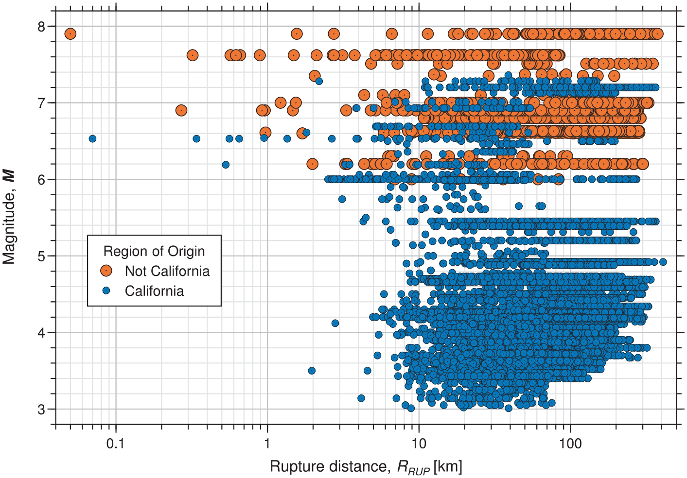
Magnitude–distance distribution of data used to develop the Chiou and Youngs (2014) GMM.
We believe that it is, therefore, still more appropriate to define a suite of source, path, and site parameters that are consistent with the backbone GMM—which may, in some sense, correspond to a pseudo-region—rather than bring in additional uncertainty related to any misfit between this pseudo-region and average conditions in the assumed host region of California. The objective is to adjust the backbone model to match the target-region characteristics and for this purpose the actual provenance of the backbone GMM is not important, provided that the host-region parameters collectively provide simulations that are a very good approximation to the predictions from the empirical model. Another advantage of determining a suite of inverted parameters that are compatible with the backbone GMM is that it allows constraints to be applied that facilitate the application of the subsequent adjustments. For example, the geometric spreading can be modeled to mimic the spreading implicit in the backbone GMM, whereas published studies reporting source, path, and site parameters for the host region may have assumed different spreading functions, which would then need to be accounted for in applying an adjustment for anelastic attenuation. In addition, the inversion can focus on matching the backbone GMM in the magnitude and distance ranges of most relevance to the PSHA integrations for the target site. Moreover, for this specific application, we are fortunate to have access to a
Inverting the CY14 GMM
Mathematical framework
Within the random vibration theory (RVT) framework, response spectral ordinates for a given natural period,
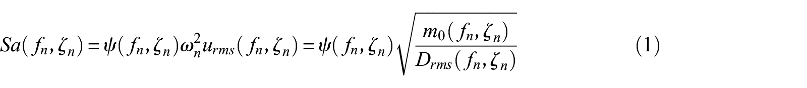
where
The zeroth moment is computed using the Fourier amplitude spectrum (FAS) of the oscillator’s displacement response
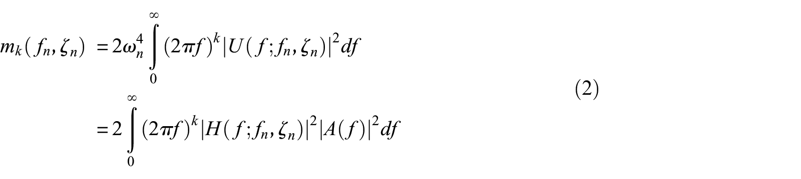
with
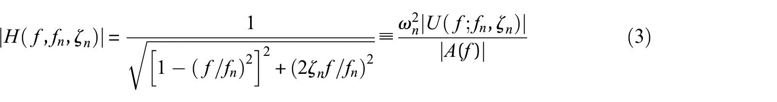
Note that this frequency response function differs slightly from that in the study by Boore (2003) as it embeds the influence of

The overview article of Boore (2003) provides detailed descriptions of these components, including a number of alternative representations that can be used for the source spectrum.
In this study, the primary objective is to obtain a set of FAS parameters that can be used for making comparisons against equivalent parameter sets inverted from empirical data in some target region. Such data are overwhelmingly dominated by recordings of rupture scenarios for which a simple point-source representation of the earthquake source is appropriate. Comparisons between host-region and target-region FAS parameter sets are greatly facilitated if the same parametric formulation is adopted. In addition, with the consideration of an appropriate distance metric, a simple point-source spectrum can also represent motions from larger events that will often be considered within hazard calculations (Boore, 2009). Therefore, while the CY14 GMM is applicable for very large events where double-corner frequency source spectra (Atkinson and Silva, 2000; Boore et al., 2014) can perform well, the source spectrum used in this study is a relatively simple single-corner frequency

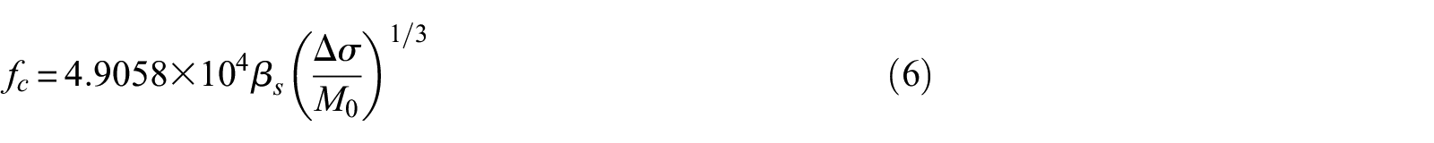
The corner frequency,
The term

with
The path scaling is comprised of geometric spreading,

The geometric spreading functions considered will be discussed subsequently, as will the choice of distance metric
Finally, the site response
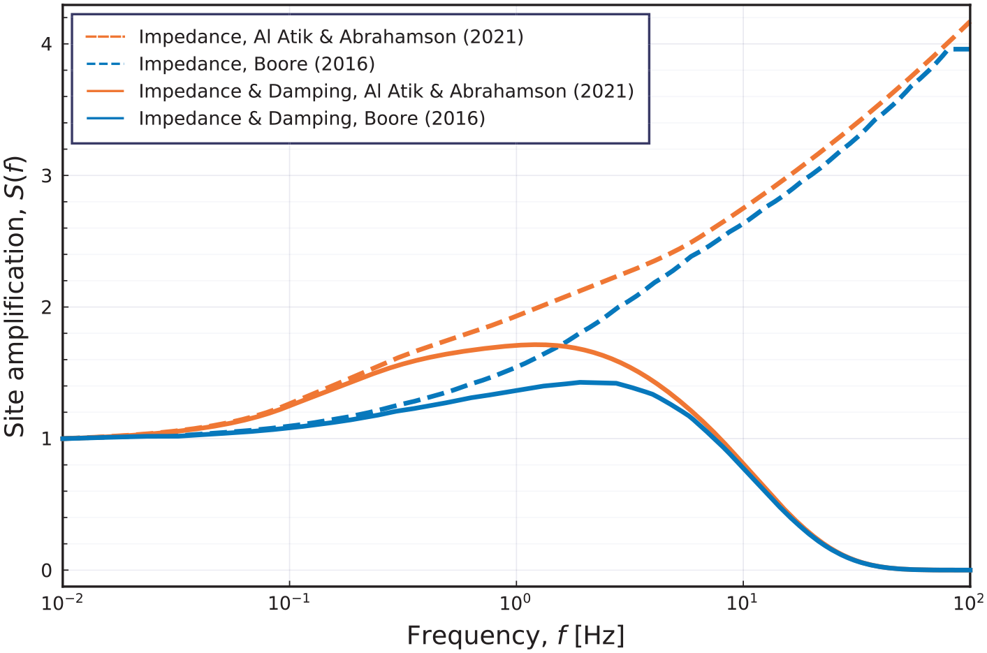
Impedance effects and overall site response. The model of Al Atik and Abrahamson (2021) is used to constrain
As noted in the previous section, we ideally want model-specific rather than host region–specific parameters, and Figure 2 demonstrates the potential implications of this point. In the absence of the Al Atik and Abrahamson (2021) model, an obvious choice to constrain the impedance effects within
The remaining terms of Equation 1 yet to be defined are

where

where
Finally, the peak factor
All terms of Equation 1 have now been defined, and this set of equations collectively define the procedure for computing a response spectral ordinate via the RVT procedure. As can be seen, a number of components are constrained within the framework. Specifically, the path duration and
In addition, while not explicitly noted in the equations presented previously, all terms of Equation 1 depend on variables that characterize the rupture scenario, such as magnitude, distance, and depth. These independent variables, along with
To identify the optimal FAS parameters, we solve for the
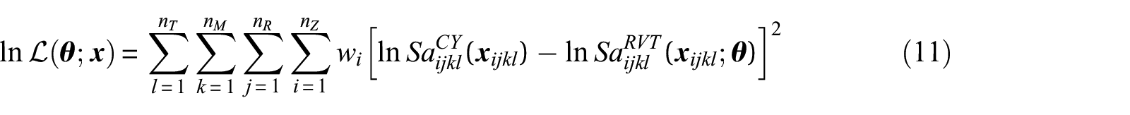
The summation over the indices
The weighted sum-of-squares expression in Equation 11 is essentially proportional to the log-likelihood function. As such, estimates of the standard errors and covariances among the FAS parameters can be computed using the Cramér–Rao bounds and the Fisher information matrix (Stafford, 2019). The Cramér–Rao bounds define the covariance matrix of the parameters

where
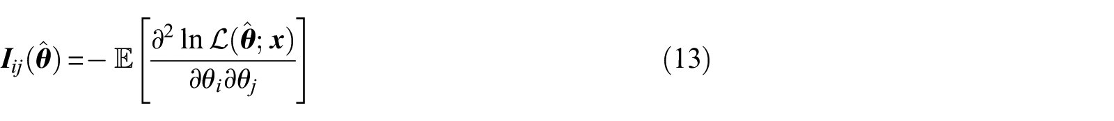
That is, the information matrix is the expectation of the Hessian matrix evaluated at the optimal parameter estimates. The computation of these mixed second-order partial derivatives for the mathematical framework presented throughout this section appears to be a formidable undertaking. However, like the gradients required for the optimization procedure, the Hessian matrix is readily evaluated using exact automatic differentiation via ForwardDiff.jl (Revels et al., 2016), as StochasticGroundMotionSimulation.jl was developed with this functionality in mind.
Parameter space
It is well known that significant parameter correlations can be encountered when performing Fourier spectral inversions (Boore, 2012; Boore et al., 1992). For this reason, inversions of empirical Fourier spectra are generally conducted in a sequence of steps in the hope of decoupling potential dependencies, as discussed in detail by Abercrombie (2021). When working with empirical data, the parameter trade-offs that are observed arise from multiple sources. Although each of the Fourier spectral parameters introduced in the previous section plays a distinct role in influencing either the amplitude or shape of spectra, the combination of the variability in Fourier spectral ordinates and the bandwidth limitations of recording instruments dictates that their unique role can rarely be isolated. Compounding this issue is the fact that the rupture scenarios represented within empirical databases impose an implicit weighting upon certain parameters over others. For example, many empirical datasets are dominated by recordings of small-magnitude events at large distances (Figure 1). Such scenarios produce recordings with a limited usable bandwidth at relatively high frequencies where the influence of
When inverting a response spectral GMM, there are different challenges to address to limit parameter correlations. The two primary issues relate to how the parameter space is sampled, and how the influence of FAS parameters manifests for response spectral ordinates (Bora et al., 2016; Stafford et al., 2017). To ensure that constraint can be imposed upon each FAS parameter of interest, it is important to sample the parameter space of independent variables to include rupture scenarios for which the loss function of Equation 11 exhibits the greatest sensitivity to each parameter.
The value of the loss function in Equation 11 depends on the particular rupture scenarios and periods that are considered. For any given set of
To explore and aid the design of the parameter space, formal sensitivity analyses were conducted. Starting with some initial estimates of parameter values,

This expression determines how a percentage change in
Figure 3 shows the relative sensitivities to four key FAS parameters for short (

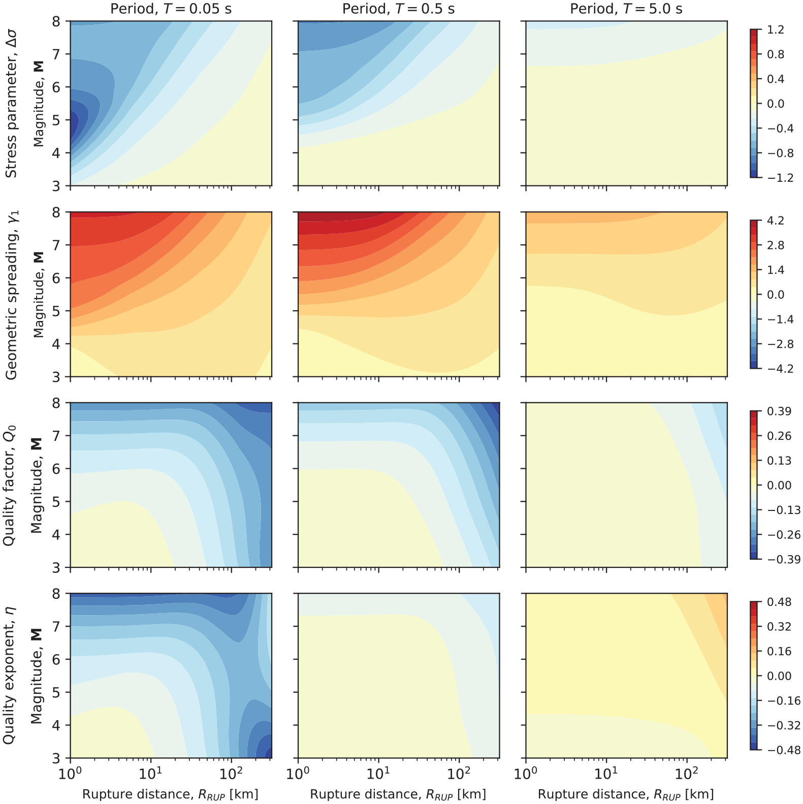
Relative sensitivities,
In Equation 15, the equivalent point-source distance
Consideration of figures like those shown in Figure 3 ensures that the
Similar considerations can be used to isolate the role of other parameters. For example, the left column of Figure 3 shows that
In addition to the above considerations, it is also important to ensure that the inverted parameter set leads to RVT predictions that mimic the CY14 GMM over a broad range of scenarios for which this GMM is applicable. If good performance over the full range of applicability is not obtained, then complications can arise when developing host-to-target adjustments as a result of extrapolation issues.
After considering the above constraints, a very comprehensive set of 7,140 magnitude–distance depth scenarios was defined. For each of these scenarios, a set of 20 periods were considered. As a result, for every evaluation of Equation 11, 142,800 RVT calculations were performed (as well as the simultaneous computation of partial derivatives with respect to each considered FAS parameter). Naturally, within the optimization process, Equation 11 is evaluated a large number of times as we move from initial parameter estimates toward the final converged solution. Formally, the optimization is terminated when the relative tolerance in estimates of
The full specification of
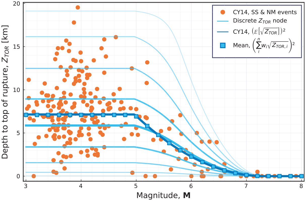
Discrete depth distribution used in the definition of the parameter space. The empirical data used for the model development are shown using circular markers. The dark solid line shows the expected depth model of CY14, while light shaded lines show nodes of the discrete depth distribution. The square markers indicate the weighted mean of these discrete depths, confirming their consistency with CY14.
Note that the full factorial combination of magnitude, distance, and depth values leads to 8,820 rupture scenarios. The lower number (7,140) of scenarios actually used arises because the depth distribution collapses to a singular value for the largest events, that is, the depth to the top of rupture for very large events is assumed to be zero (Figure 4).
Host CY14 GMM for inversions
Because the source within the FAS model is treated as an equivalent point source, it is not possible to explicitly model effects associated with style of faulting and fault-finiteness (such as hanging-wall effects and directivity). For this reason, the rupture scenarios that are considered all correspond to vertical strike–slip ruptures, and directivity effects are ignored. This modeling decision effectively simplifies the CY14 model by rendering many of the functional terms of the model redundant. For vertical strike–slip ruptures, ignoring directivity effects (setting
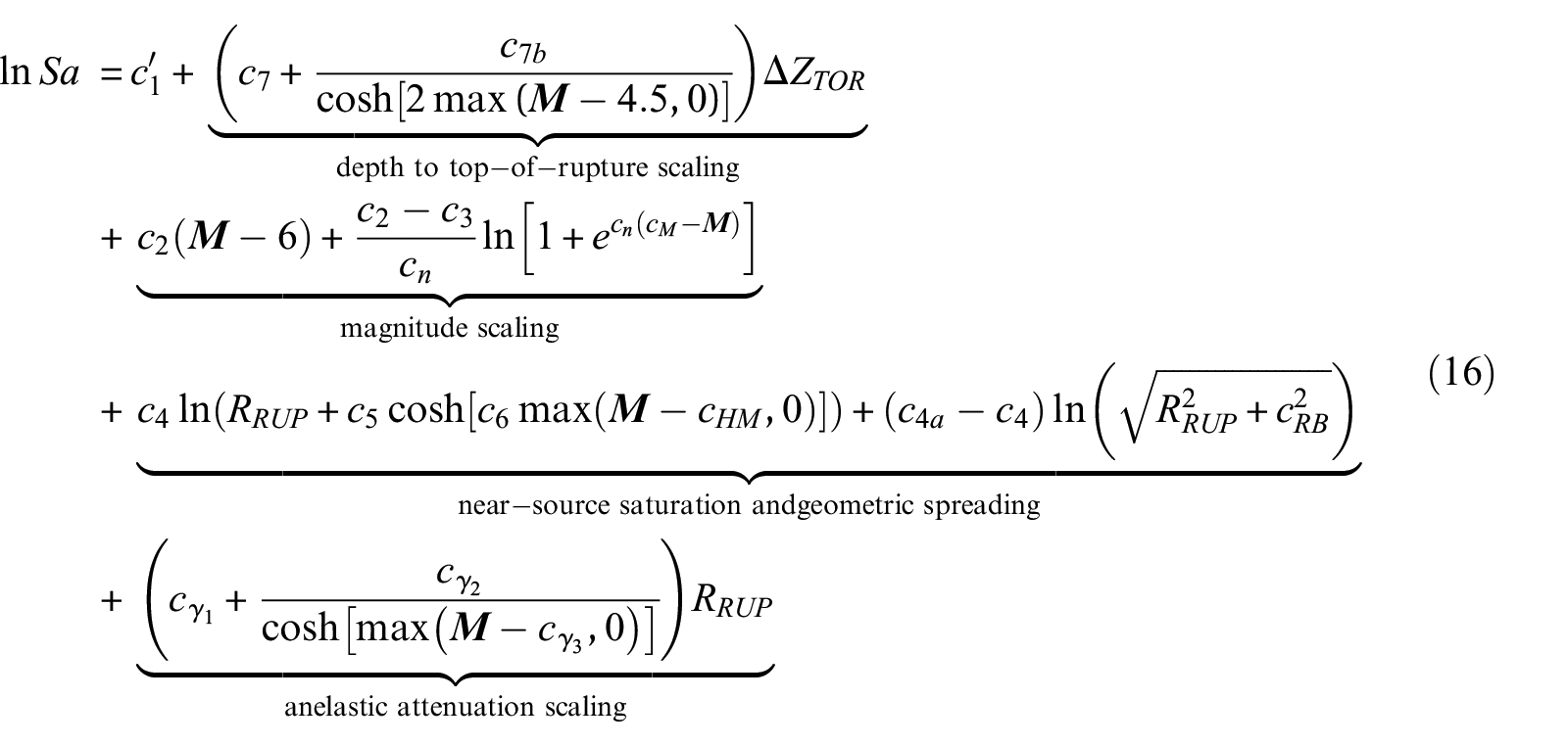
where the
In Equation 16, the distinct functional terms that relate to
We can also see that the geometric spreading functional form shares a lot in common with the function shown previously in Equation 15. The equivalent point-source distance,

where Boore and Thompson (2015) use

with
Inversion results
A challenge often faced when developing model adjustments is the reconciliation of “apparent parametric” and “real physical” differences that arise from considering different magnitude ranges in the host and target regions. In particular, target region FAS parameter sets are often inferred from recordings of small magnitude events, while potential host regions are generally considered because they have empirical constraint for larger rupture scenarios of greater relevance to hazard calculations. It is, therefore, important to ensure that the inversion of the CY14 GMM is robust for small magnitude events, and that any magnitude dependence in the FAS parameters is adequately modeled. When this is done successfully, differences in host and target region parameter sets obtained over the small magnitude range can be appropriately scaled to corresponding differences at larger magnitudes (assuming the physical FAS model is appropriate).
As a result, the first step of the inversion procedure is to investigate any magnitude dependence of the FAS parameters by performing inversions for specific magnitude values. This first step is discussed in the following section, and informs the parameterization of the full inversions presented subsequently.
Initial magnitude-dependent scaling
For a fixed value of magnitude, it can be appreciated that many elements of the functional complexity within Equation 16 disappear. To mimic the functional form of Equation 16, a single-corner source spectrum was adopted, with the stress parameter made a function of the relative depth to the top-of-rupture,

where

with
Inversions are performed for the periods, distances, and depths previously presented in the Parameter Space section, and for individual magnitudes from 3.0 to 8.4 in 0.2 unit increments. The results of these initial inversions are presented in Figure 5. In all cases, both the parameter estimates and the associated standard errors are shown. Figure 5a shows that stress parameter estimates initially grow exponentially with magnitude, up to
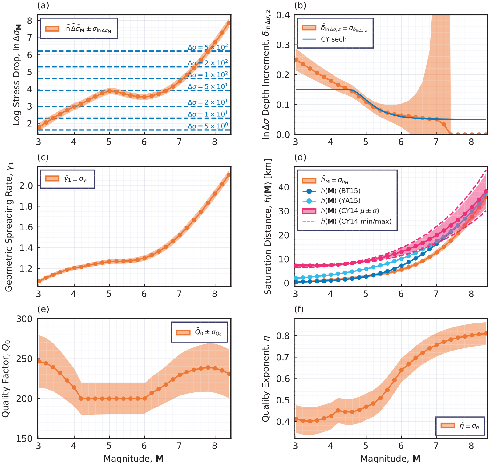
Variation of FAS parameters with magnitude, from magnitude-specific inversions. (a) Logarithmic stress parameter estimates are shown, along with annotated
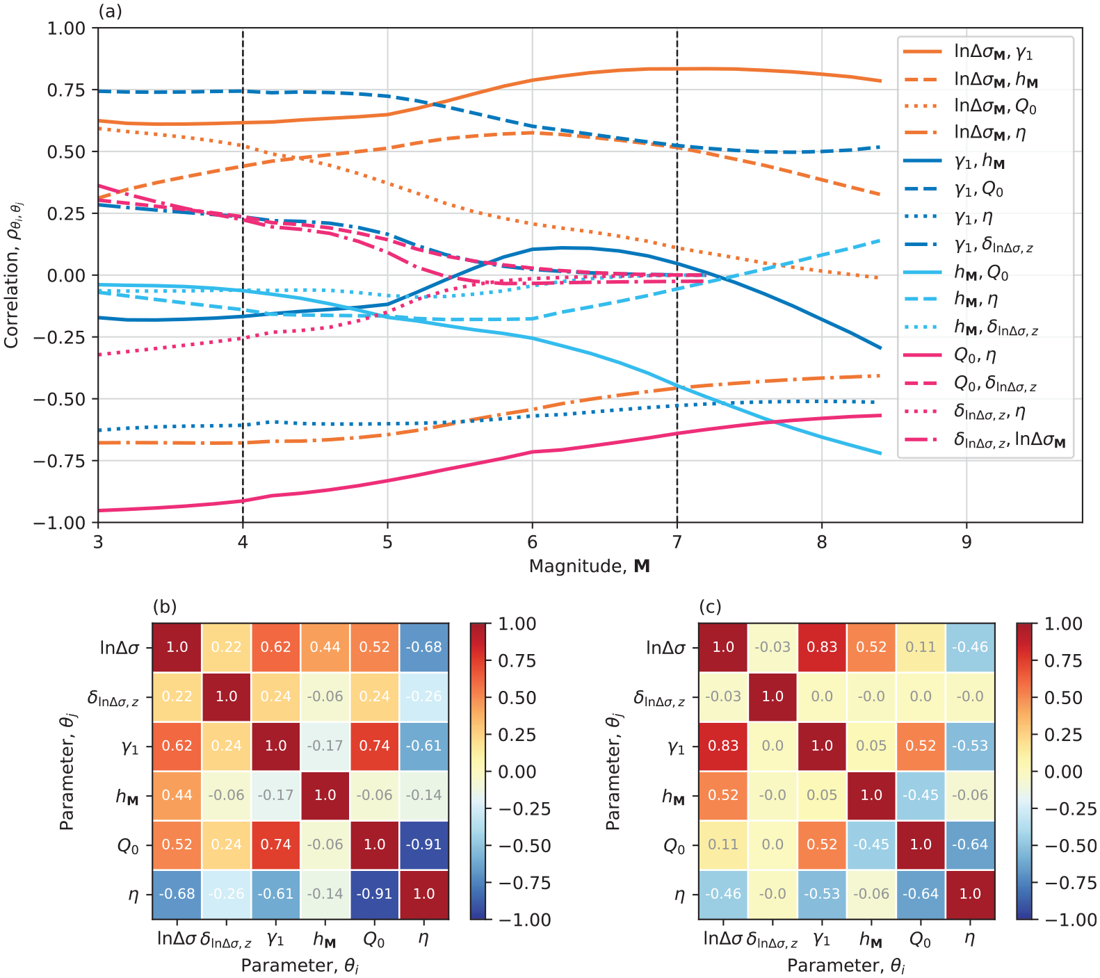
Parameter correlations from magnitude-specific inversions. (a) The variation of parameter correlations with magnitude are shown. Vertical gray dashed lines correspond to the magnitudes for which the correlation matrices are plotted in (b) and (c).
Figure 5b shows the influence of
Figure 5d compares multiple models for the near-source saturation distance,
Finally, Figure 5e suggests that
The correlation values in Figure 6 are encouraging in that we do not observe parameter combinations where the correlation stays very strong (positive or negative) over the full magnitude range. The most extreme correlations correspond to the combinations of
Optimal parameterization
Following the magnitude-specific inversions discussed in the previous section, a number of alternative parameterizations for the full inversion were considered. These alternatives were judged on the basis of their “scores,” as defined by Equation 11, and upon their general ability to mimic the scaling within the CY14 GMM in a parsimonious way. The latter characteristic was judged from visual inspection of diagnostic plots, but is also clearly related to the formal metric provided through Equation 11.
Note that while physical reasoning influences the selected parameterization in part, the ultimate goal is to derive a set of FAS parameters that reproduce the scaling embedded within the CY14 GMM. It must also be recalled that the specification of the FAS model is only one part of the overall inversion, as the site response, duration models, and peak factor model are all constrained. The specific scaling embedded within these RVT components also influences how the FAS model should behave. For example, Equation 1 shows that spectral amplitudes scale with both
For the full inversion, the stress parameter was defined to include explicit magnitude dependence for small magnitudes, and to also embed the effects of the depth to top of rupture. The magnitude dependence largely offsets the near-source saturation distance of the CY14 GMM, as previously discussed. The scaling with
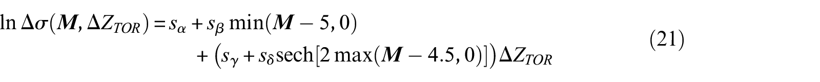
where
Geometric spreading is defined in Equation 20, with the equivalent point-source distance defined as:

and the near-source saturation distance coming from:

where
Within the inversion, a nonlinear constraint is imposed upon the combination of
Finally, the quality exponent within the anelastic attenuation filter is modeled as magnitude dependent, based on the results presented in Figure 5f. The distance metric used within the anelastic attenuation filter is

with
In total, the optimal parameterization requires solving for 13 free parameters. The resulting parameter estimates and associated standard errors are presented in Table 1.
Estimates and standard errors for the optimal FAS parameters
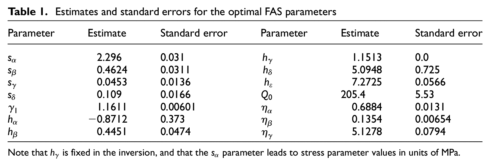
Note that
Convenience parameterization
While the optimal parameterization of the previous section is simple to implement in StochasticGround vMotionSimulation.jl, existing workflows based on alternative software may not be able to accommodate this parameterization. In particular, the mixing of distance metrics in Equation 20 and the magnitude dependence of
This alternative parameterization closely follows the geometric spreading formulation by Boore (2003), and makes use of
The form of the geometric spreading adopted is trilinear in
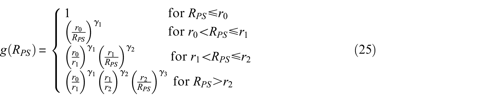
with
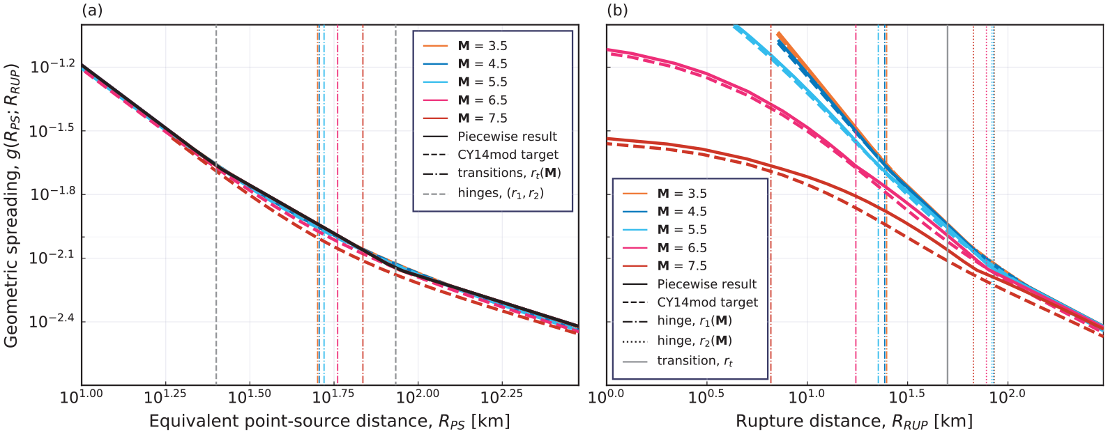
Comparison of the geometric spreading functions of Equations 20 and 25 (“CY14mod target” shows the scaling of Equation 20, while “Piecewise result” corresponds to Equation 25). (a) The spreading function for various magnitudes against the equivalent point-source distance is shown, while (b) shows the same function plotted against the rupture distance. Vertical lines in both panels correspond to either hinge distances,
It is not possible to obtain perfect agreement between the two path-scaling variants. A key challenge is the mixing of distance metrics, with hinge distances being defined in terms of
With the hinge distances defined at
Parameter estimates and standard errors for the convenience parameterization (geometric spreading defined according to Equation 25, magnitude-independent
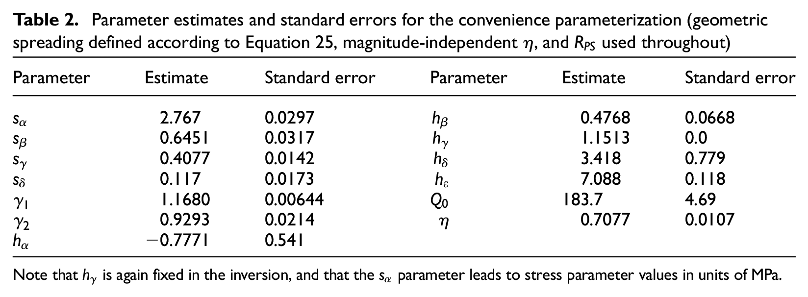
Note that
Model performance
The performance of both the optimal and convenience models are demonstrated through visual comparison with CY14 in Figures 8 to 10. In all cases, the dashed lines represent the target CY14 model predictions, the solid lines correspond to the optimal FAS model, and the dotted lines are for the convenience model.
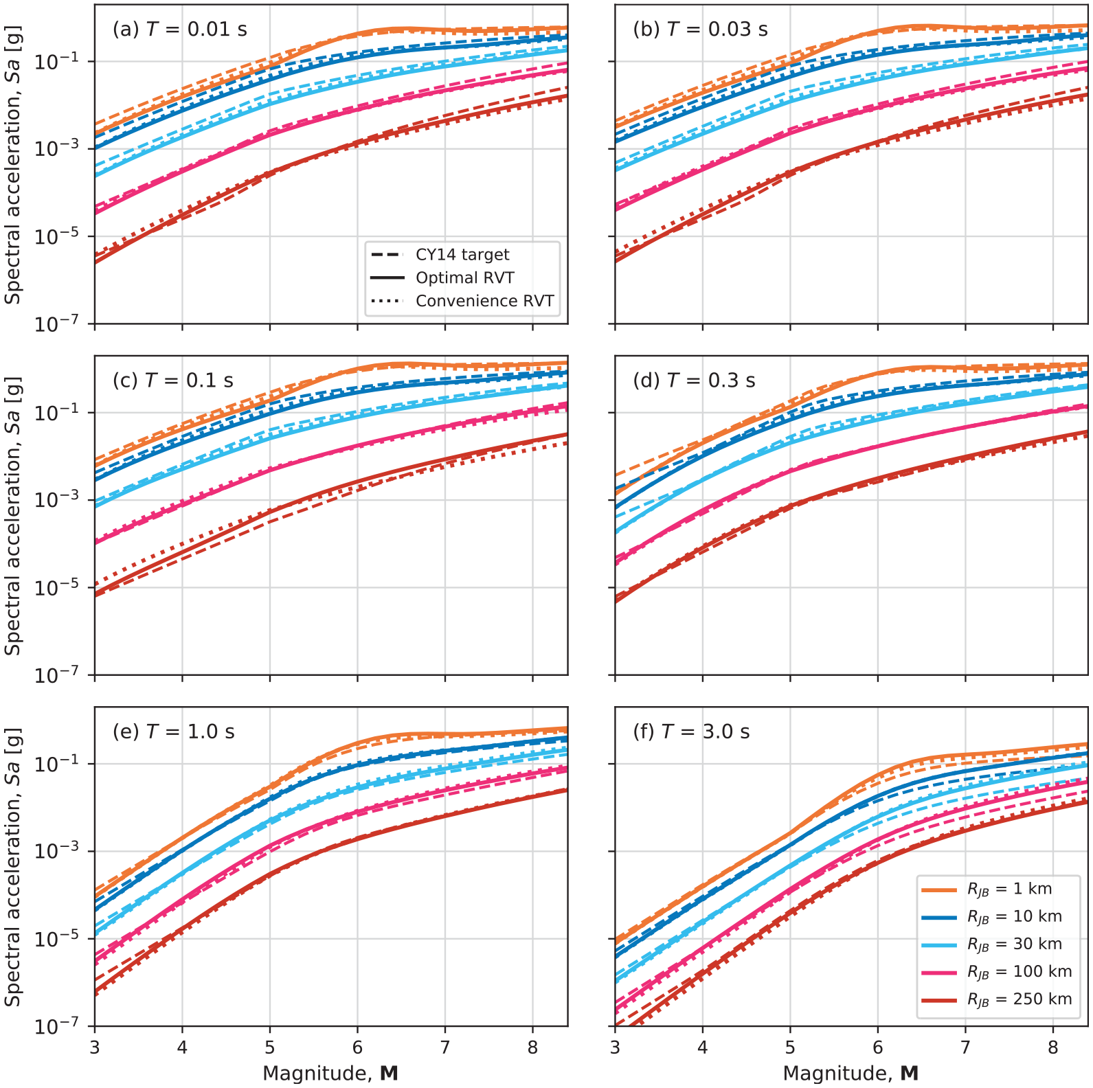
Comparison of magnitude scaling in the CY14 GMM and the two RVT-based models defined by the parameters in Tables 1 (“Optimal RVT”) and 2 (“Convenience RVT”). (a)–(f) Each show the scaling for a particular period. The legends in (a) and (f) apply to all panels.
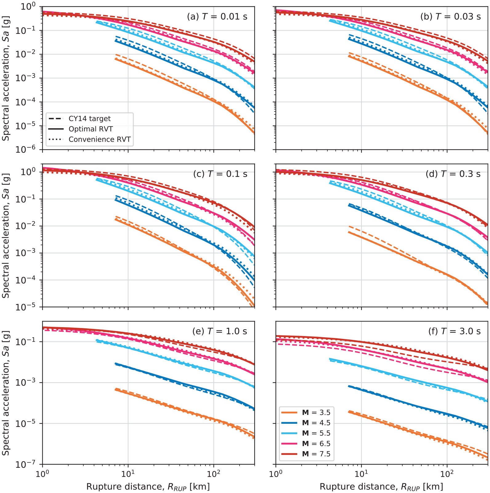
Comparison of distance scaling in the CY14 GMM and the two RVT-based models defined by the parameters in Tables 1 (“Optimal RVT”) and 2 (“Convenience RVT”). (a)–(f) Each show the scaling for a particular period. The legends in (a) and (f) apply to all panels.
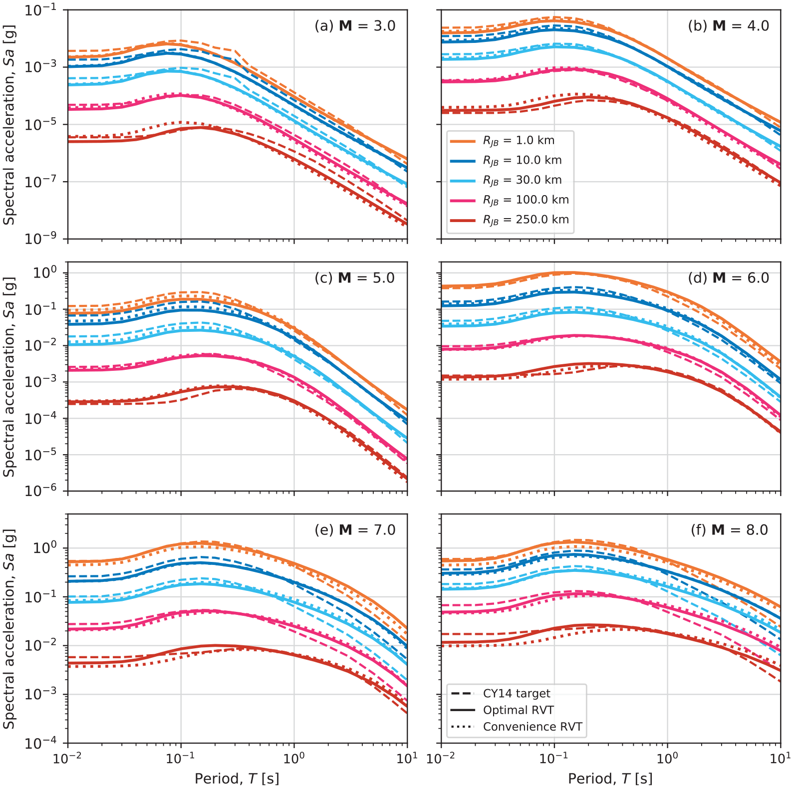
Comparison of spectral scaling in the CY14 GMM and the two RVT-based models defined by the parameters in Tables 1 (“Optimal RVT”) and 2 (“Convenience RVT”). (a)–(f) each show the scaling for a particular magnitude. The legends in (a) and (f) apply to all panels.
Figure 8 shows the magnitude scaling of the models for six periods that span the range of typical engineering interest. The most obvious feature of interest in this figure is the difference in magnitude scaling at the very short distance of
For all other periods and distances, we generally observe a close agreement between all three sets of model predictions. In judging the performance of the RVT-based predictions, it is important to keep in mind that the primary use of the RVT parameterization is to develop host-to-target model adjustments. In this context, absolute differences in amplitude are arguably less important than achieving a good similarity of the “shapes” of the curves. Furthermore, “local” issues like the magnitude scaling at
It is also noteworthy that the loss in performance associated with using the convenience parameterization over the optimal parameterization is not visually obvious from Figures 8 to 10. Figure 9, focusing upon distance scaling, should be expected to highlight differences between these two RVT-based models most clearly. However, there are many rupture scenarios (often at relatively short distances) where the convenience parameterization outperforms the optimal model. Where the optimal model tends to show that superior performance is at large distances and relatively short periods. For these scenarios, the use of magnitude-dependent
Part of the reason why the change in geometric spreading formulation is not so crucial is that despite Equation 20 attempting to mimic the functional form of CY14, the overall path scaling of
Figure 9 shows predictions obtained using
The comparison of spectral scaling in Figure 10 shows that we achieve very good agreement in both spectral shape and absolute amplitude for the small-to-moderate magnitude scenarios. This is largely to be expected given that the point-source approximation should work most effectively for these magnitudes. In Figure 10e and f, we see that the RVT-based models have difficulty replicating the spectral shape of CY14. In particular, at long periods, the rate of spectral decay with period is stronger for CY14 than in the RVT models. This portion of the response spectrum is primary controlled by low frequencies in the Fourier domain where our FAS model has relatively few degrees of freedom. In particular, once a single-corner source spectrum is adopted, we have very limited control over these low-frequency FAS ordinates. At short periods and large distances, we also have challenges replicating the spectral shape for large magnitudes. Here, the role of the magnitude-dependent
The degree of agreement between the CY14 target and the RVT-based predictions shown in Figures 8 to 10 can be slightly misleading as a result of plotting predictions over multiple decades. For this reason, Figures 11 to 13 show the relative performance of the optimal and convenience models through ratios with respect to the CY14 target. In all cases, values of unity correspond to a perfect match with the CY14 prediction. While these figures demonstrate that the RVT-based models are generally within 50% of the CY14 target, it is clear that there are local variations in the degree of agreement with respect to magnitude. To put this into some perspective, Al Atik and Youngs (2014) showed that the model-to-model standard deviation among the NGA-West2 GMMs is on the order of 0.2 natural log units—corresponding to a factor of ≈20% (with the model-to-model range being larger). For the distance ratios in Figure 12, the ratios are largely flat to beyond 100 km, before the differences in anelastic attenuation play a stronger role. For the spectral ratios, Figure 13 shows that for most distances, the ratios are also relatively flat at short periods (indicating similar spectral shape to CY14), but that departures increase at longer periods.
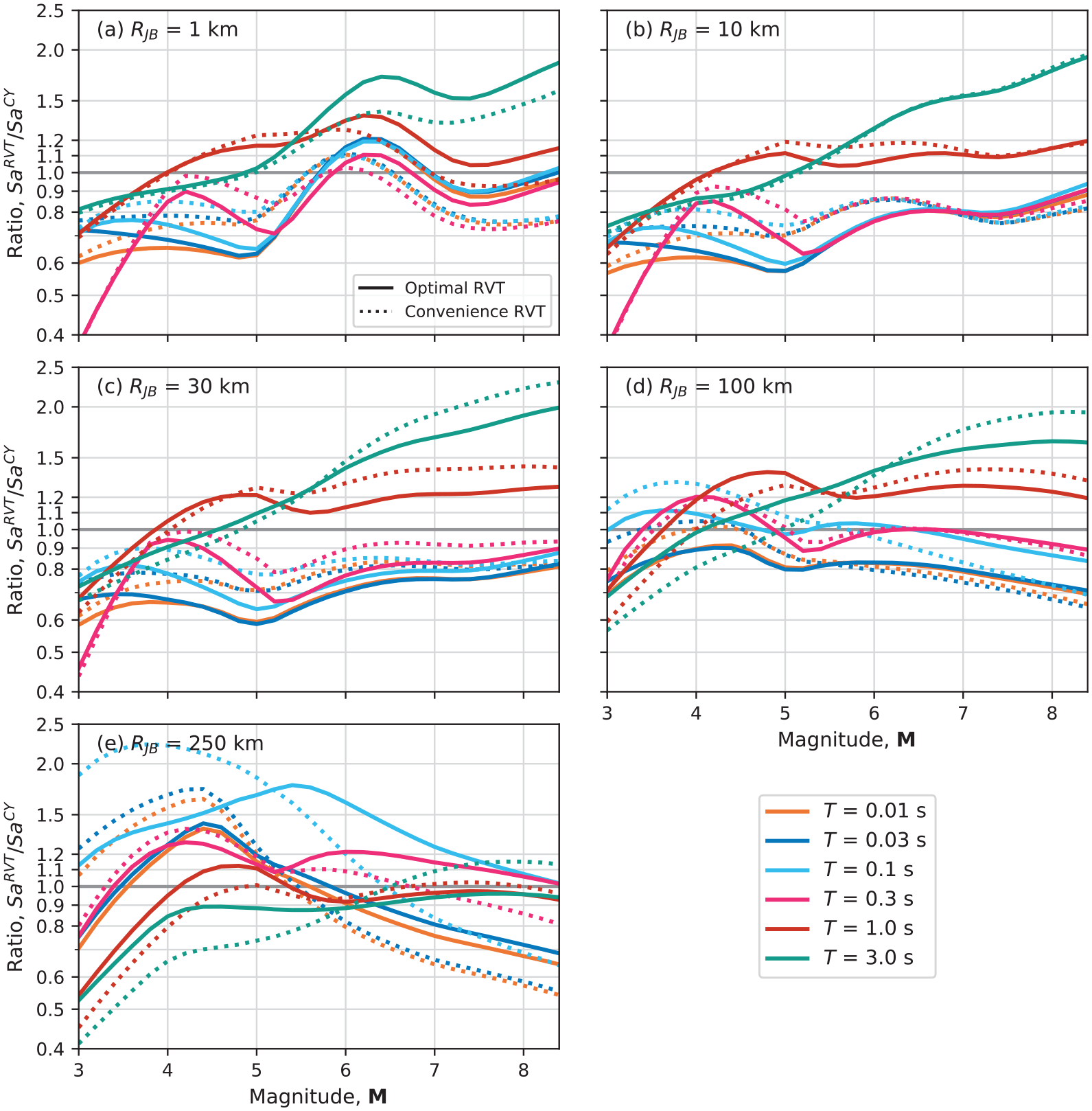
Ratios of the RVT-based predictions to the CY14 target with respect to magnitude, for a number of distances and periods.
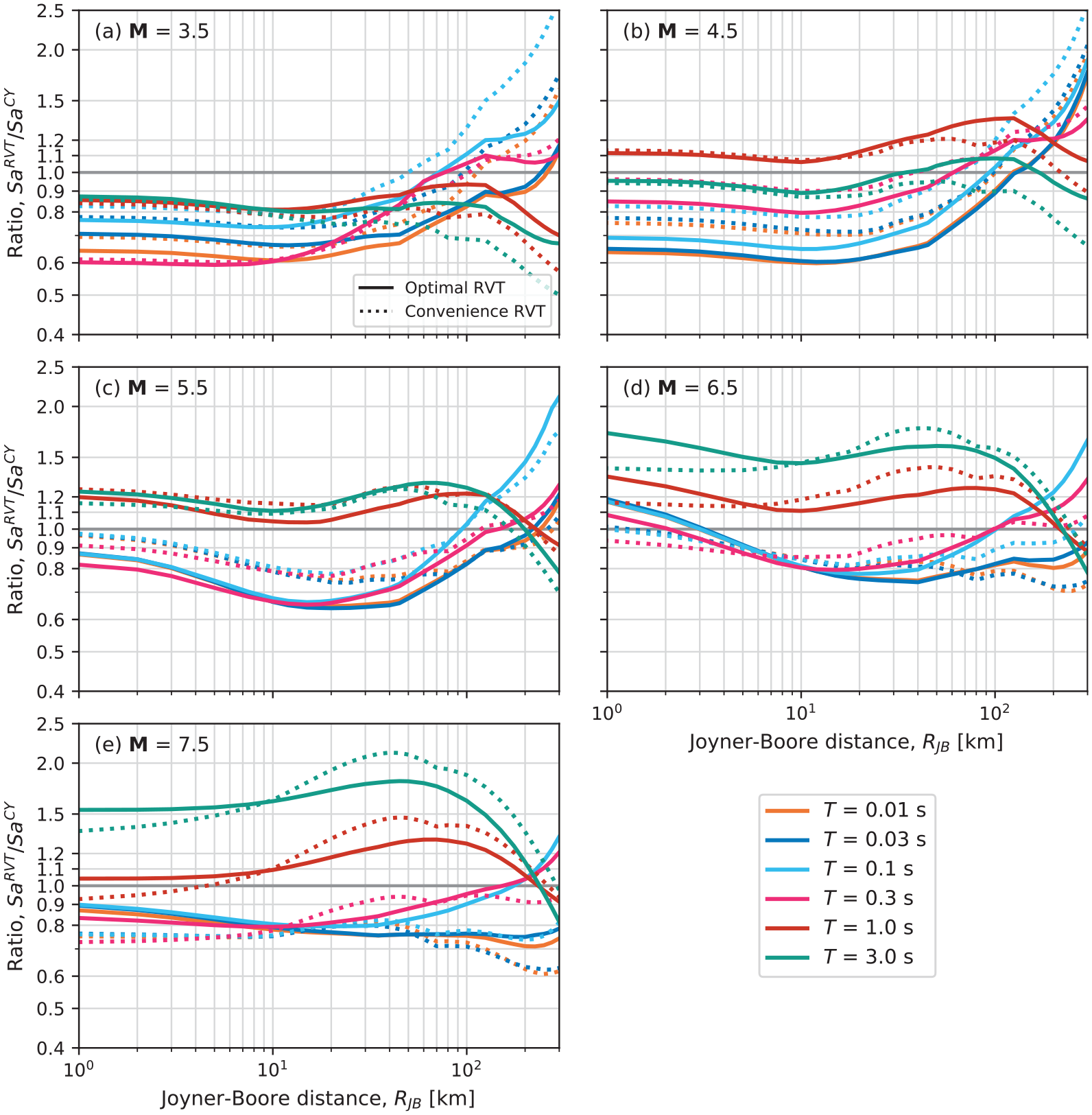
Ratios of the RVT-based predictions to the CY14 target with respect to distance, for a number of magnitudes and periods.
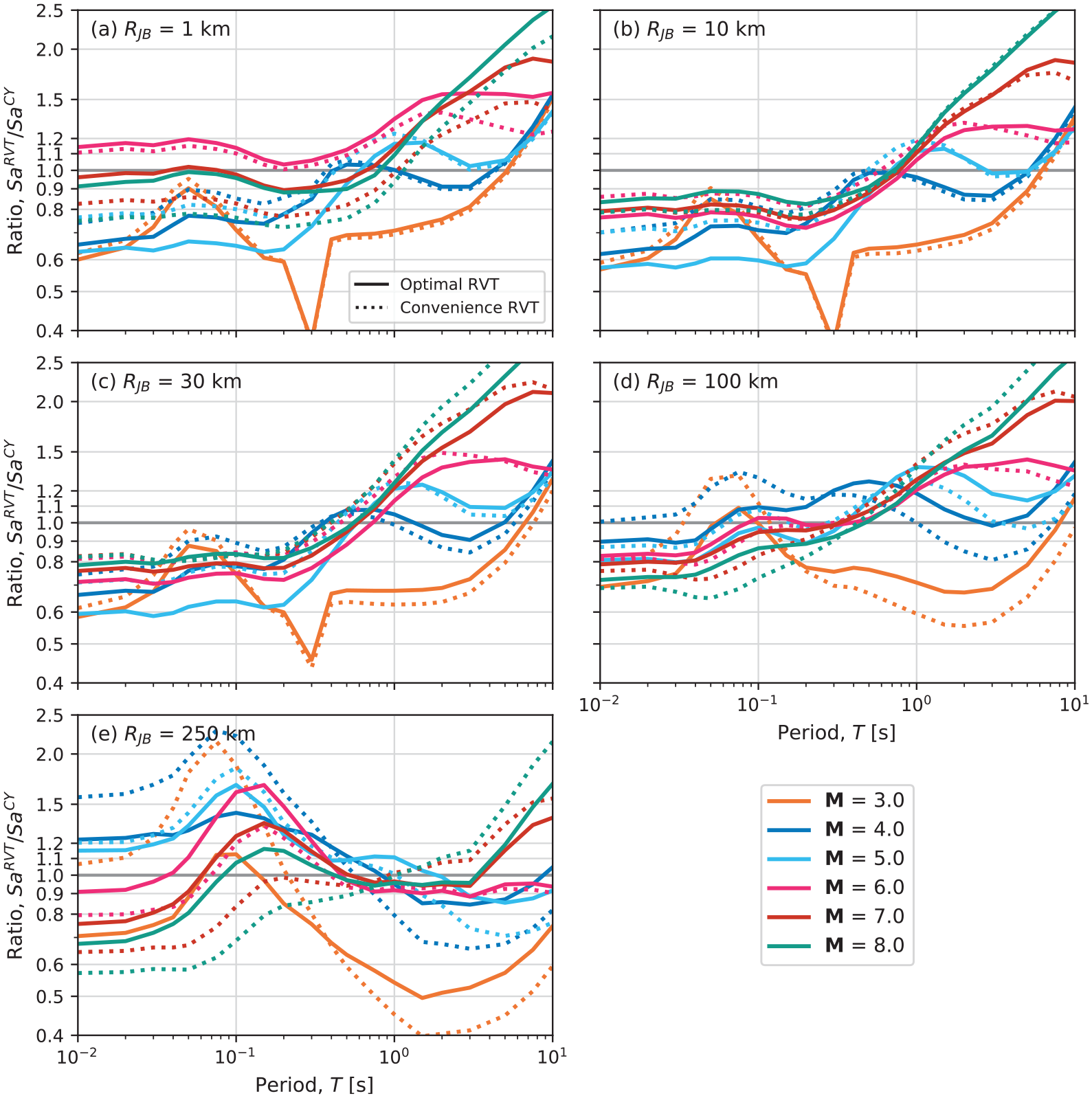
Ratios of the RVT-based predictions to the CY14 target with respect to period, for a number of magnitudes and distances.
In general, consideration of Figures 11 to 13 indicate that both the optimal and convenience parameterizations face similar challenges in replicating the scaling of the CY14 model. Comparisons of corresponding pairs of curves in these figures tends to show that the optimal model (solid lines) is slightly closer to unity than the convenience model (dotted lines), on average. However, it is also clear from the complete set of Figures 8 to 13 that the optimal parameterization is not drastically superior to the more familiar convenience parameterization.
As noted previously, the primary purpose of these inversions is to facilitate host-to-target model adjustments, and it is important to keep in mind where, in magnitude–distance space, empirical constraint for the target region tends to come from. Generally speaking, for the small-to-moderate magnitudes and intermediate-to-long distances of greatest practical importance, both the FAS parameterizations do a good job of replicating the absolute amplitude and scaling of the CY14 GMM.
Discussion and conclusion
In this article, we have presented host-region parameters that are broadly consistent with the CY14 GMM, with the intention of facilitating the application of a backbone GMM approach to constructing a logic tree for use in PSHA in a region of crustal seismicity. The CY14 accounts for scaling features that cannot be captured through standard parameterizations of the Fourier spectrum based on point-source seismological theory, and it is never the intention to perfectly match the CY14 predictions using the inverted FAS parameter set. However, it is important to achieve as close a match as possible so that model adjustments derived within the HEM framework do not distort the general scaling of the CY14 model in undesirable ways when it is adapted for application in the target region. In addition, it is important to capture magnitude dependencies of the FAS parameters so that parametric comparisons between the host model and the target region relate to similar rupture scenarios.
If the approach and these parameter suites presented in the article are accepted, then the task of developing a ground-motion logic tree can focus exclusively on determination of the target-region parameters. This is likely to be achieved through a combination of in situ site measurements and analyses of ground-motion recordings from the target region, including estimation of the uncertainty associated with each of the target-region parameters. The source and path differences can be accommodated through direct adjustments to the appropriate coefficients of CY14, or by developing adjustment factors using the HEM framework. The site adjustment can be made in one of two ways, either through the application of
Footnotes
Acknowledgements
We are grateful for three comprehensive reviews provided by John Douglas, Sreeram Kotha, and an anonymous reviewer that helped to improve the manuscript.
Authors’ note
The work presented herein has also been motivated by the requirements of site-specific PSHA projects for nuclear facilities and has benefited greatly from the exchanges with participants in those projects. In particular, the work evolved within the SSHAC Level 3 PSHA for the INL site and was enriched by exchanges with Linda Al Atik, Bob Darragh, Albert Kottke, Jim Kaklamanos, Adrian Rodriguez-Marek, and Walt Silva.
Declaration of conflicting interests
The author(s) declared no potential conflicts of interest with respect to the research, authorship, and/or publication of this article.
Funding
The author(s) disclosed receipt of the following financial support for the research, authorship, and/or publication of this article: This work was partially funded by the Idaho National Laboratory (INL) through the US Department of Energy Idaho Operations Office contract DE-AC07-05ID14517.