Integration of rupture directivity models for the US National Seismic Hazard Model

Abstract

Several rupture directivity models (DMs) have been developed in recent years to describe the near-source spatial variations in ground-motion amplitudes related to propagation of rupture along the fault. We recently organized an effort toward incorporating these directivity effects into the US Geological Survey (USGS) National Seismic Hazard Model (NSHM), by first evaluating the community’s work and potential methods to implement directivity adjustments into probabilistic seismic hazard analysis (PSHA). Guided by this evaluation and comparison among the considered DMs, we selected an approach that can be readily implemented into the USGS hazard software, which provides an azimuthally varying adjustment to the median ground motion and its aleatory variability. This method allows assessment of the impact on hazard levels and provides a platform to test the DM amplification predictions using a generalized coordinate system, necessary for consistent calculation of source-to-site distance terms for complex ruptures. We give examples of the directivity-related impact on hazard, progressing from a simple, hypothetical rupture, to more complex fault systems, composed of multiple rupture segments and sources. The directivity adjustments were constrained to strike–slip faulting, where DMs have good agreement. We find that rupture directivity adjustments using a simple median and aleatory adjustment approach can affect hazard both from a site-specific perspective and on a regional scale, increasing ground motions off the end of the fault trace up to 30%–40% and potentially reducing it for sites along strike. Statewide hazard maps of California show that the change in shaking along major faults can be a factor to consider for assessing long-period $(>1\mathrm{s})$ near-source effects within the USGS NSHM going forward, reaching up to 10%–20%. Finally, we suggest consideration of minimum parameter ranges and baseline requirements as future DMs are developed to minimize single approach adaptations to enable more consistent application within both ground motion and hazard studies.

Introduction

Near-source ground-motion amplitudes exhibit a variety of spatial variations that are not currently included in many seismic hazard studies. One of these phenomena is rupture directivity, where ground motions vary as a function of azimuth and distance from the source, generally modeled by the station’s location with respect to both rupture propagation and slip direction. Rupture directivity, often abbreviated as just “directivity,” is primarily a near-source effect of earthquake rupture whereby seismic energy is focused in the direction of rupture propagation due to the constructive interference of radiated waves as the rupture propagates along the fault near the shear (SH)-wave velocity (Somerville et al., 1997). The intensity of this amplification at a given location is observed to depend on the azimuth of the site relative to the rupture propagation direction with reference to slip direction along the fault, combined with the distance from the source. Despite the fact that directivity effects can be a substantial fraction of ground-motion spectral acceleration (SA) estimates, these spatial adjustments have not been explicitly incorporated into the US Geological Survey’s (USGS) National Seismic Hazard Model (NSHM) of probabilistic seismic hazard assessment (PSHA) (Petersen et al., 2014; Petersen et al., 2020) Thus, the USGS has recently initiated a coordinated effort toward incorporating rupture directivity models (DMs) into the NSHM software, focused on assessing the effect of rupture directivity adjustments to seismic hazard. We consider external advice at public workshops from directivity modelers, engineers, and practitioners to help guide implementation decisions and characterization of seismic hazard adjustments.

We expand upon recent studies (Donahue et al., 2019; Spudich et al., 2014) by examining a hypocenter-independent approach for the implementation of directivity effects into PSHA, a more computationally efficient approach than looping over hypocenter locations within the hazard calculations. This work examines the effect from both a median and aleatory variability adjustment to the USGS NSHM, helping to assess regions where directivity effects influence hazard using complex source geometries.

This effort began by first performing a review of the models developed to describe rupture directivity phenomena and then proceeding to evaluate DM characteristics, assumptions, and prediction limitations. We synthesized several preexisting DMs to a common coding language to compute factors for scaling ground motions to evaluate both empirical and simulated data for various finite-fault conditions. We compared the strengths and weaknesses of these DMs, including their ability to model spatial variations of both strike–slip and dipping faults over a range of magnitudes and spectral periods, with a particular focus on analyzing the spatial dependence of geometrical factors that scale ground motions predicted by leading ground-motion models (GMMs). We next analyzed computational impediments toward implementation into the USGS current seismic hazard software, nshmp-haz (Powers et al., 2022). This analysis informed our decision to consider several methods outlined in the literature (Donahue et al., 2019; Spudich et al., 2014) to incorporate directivity effects into hazard calculations. We considered two end-member implementation options within a PSHA framework: (1) a median and aleatory adjustment model based on the average effect from a priori computing hypocenter-dependence and (2) incorporating hypocenter location explicitly within the hazard integral and looping over a hypocenter distribution. Ultimately, we implemented a straightforward adjustment of the median and aleatory variability to the ground-motion prediction, requiring additional fault distance terms to be implemented into the nshmp-haz code. Using this simple ground-motion adjustment, we have analyzed the effect on hazard from simple to complex faulting systems and consider this the best approach for incorporation of directivity into the next update of the USGS NSHM. We focus our efforts to fault systems where DMs have the greatest agreement between one another and are most important to hazard, such as strike–slip ruptures along high-slip rate faults, and show comparison of directivity adjustments for both this partial selection of faults and the full Uniform California Earthquake Rupture Forecast, Version 3 (UCERF3) (Field et al., 2014) fault database (excluding dip–slip ruptures). Spatial amplification is compared with hazard maps, at 475- and 2475-year return periods, through difference and ratio plots, while individual stations are viewed via the lens of uniform hazard spectra. We consider the effect of the median and aleatory variability adjustment on ground motion, evaluating the effect of standard deviation on hazard levels. We end with suggestions to ensure future DMs have common ground when computing ground-motion adjustments and the ability to enhance uniformity in application to PSHA computations.

Overview of recent rupture directivity efforts

Rupture directivity effects have long been noted in the literature to cause variations in ground-motion amplitudes not explainable with typical azimuth-independent predictor variables (to name a few: Aagaard et al., 2004; Archuleta and Hartzell, 1981; Bray and Rodriguez-Marek, 2004; Somerville, 2003; Wang and Day, 2020). This is evidenced in the seismograms recorded from large magnitude events (such as Landers: Gomberg et al., 2001, Chi-Chi: Hwang et al., 2001, Kobe: Somerville et al., 1996, Denali: Velasco et al., 2004; and Ridgecrest: Ahdi et al., 2020) that exhibit both forward and backward directivity features caused by the rupture propagation, the source radiation pattern, and polarization of seismic waves (as noted in the work by Somerville et al., 1997). This behavior is often exhibited as “pulses” in the velocity time series of stations in the forward rupture direction of both empirical and synthetic recordings (Shahi and Baker, 2014).

There have been many efforts toward modeling the effects of rupture directivity exhibited in ground-motion amplification, including consideration of specific earthquakes, scenario events, collections of empirical data, or via expressions for adjustments to GMMs (e.g. Dabaghi, 2014; Dabaghi and Kiureghian, 2014; Rodriguez-Marek and Cofer, 2009; Shahi and Baker, 2011; and Somerville, 2003). Recent reports have summarized some of the work that focuses on application to modification of ground motions (Spudich et al., 2013; Spudich et al., 2014) and implementation into PSHA models (Donahue et al., 2019). These publications outline the substantial progress achieved by the community, but they acknowledge that substantial effort remains to develop a more thorough understanding of directivity effects and integration into modern calculations of ground-motion and seismic hazard assessment. In the next section, we outline some of the models developed to characterize directivity behavior and discuss the various factors to consider for spatial adjustment of GMMs and hazard application.

Rupture Directivity Models

Numerous DMs were developed within the past two decades since Somerville et al. (1997) sought to describe the consistent features observed in ground-motion amplification aligned with rupture propagation. Spudich et al. (2014) summarize the key concepts of five of these DMs and their anticipated application within the NGA-West2 GMMs (Ancheta et al., 2014). We highlight the relevant concepts here. A key point is that even though the modelers have pursued different routes toward capturing the source characteristics of fault rupture, there is common ground among the models and how they can be incorporated into modifications accounting for near-source spatial adjustments to ground motion. For example, each method outlined (Spudich et al. 2014) (as further detailed in the work by Baker, 2007; Bayless et al., 2020; Rowshandel, 2010; Shahi and Baker, 2014; Spudich and Chiou, 2008) is generally designed to predict an adjustment factor at varying oscillator periods to the mean SA, RotD50 (as in the work by Boore, 2010). Some models also provide a directivity-related aleatory variability adjustment term that accounts for the reduced misfit to GMMs when accounting for the influence of azimuthal dependency on ground motions. This reduced misfit is theoretically GMM-dependent, but is observed to not vary substantially from model to model (e.g. Bayless et al., 2020).

These models fall into two categories: one derived via a physical “intuitive” approach (Bayless et al., 2020; Rowshandel, 2018a; Shahi and Baker, 2014) and one that use a more theoretical approach (such as the work by Spudich and Chiou, 2008). These are differentiated by whether the model is guided by empirical observations or by isochrone theory using isochrones, contours of equal velocity, relating to the velocity ratio, and points in relation to the fault plane. All of the model developers use the NGA-West2 events with finite-fault data (Ancheta et al., 2014), sometimes in combination with synthetic data, to supplement the limited empirical recordings to best-fit features not captured with azimuthally invariant GMMs. The models are limited in application, based upon the distribution of the recordings relating to magnitude, distance, and spectral period. Because the style of faulting has a large effect on the directivity spatial pattern, most modelers apply their models separately to strike–slip versus dip–slip faults, based upon the average fault rake and dip. The level of complexity varies substantially among the models, which affects the required predictor variables and the ability to fit source effects. For example, the slip and rake angle is incorporated in the work by Rowshandel (2010) (and Rowshandel, 2018a) to model oblique-slip effects that may not otherwise be captured by other models. In a later section, we illustrate how these variations cause differences in both the amplitude and spatial patterns predicted by each DM, particularly for nonvertical faults.

One concept to which all models must adhere is “centering”—ensuring that the magnitude and distance scaling of a GMM is not shifted by the introduction of directivity adjustments. Modelers have accomplished this in two different ways: (1) by subtracting off the average adjustment along “racetracks” of equal distance from the fault, a method performed by the Chiou and Spudich model, presented in the work by Spudich et al. (2014), with reference to the direct point parameter (DPP) or (2) developing a DM using ground-motion residuals (with respect to GMMs). If the residuals are centered in this second approach—so they also exhibit no bias due to magnitude/distance variation—it is assumed that the model produced will not affect the underlying mean ground-motion prediction. There has been a continual improvement of these models in the years since the first attempt to model directivity effects (Somerville et al., 1997). Within these most recent iterations, changes have focused on more accurately modeling ground-motion adjustments, most notably the handling of source dimension normalization and magnitude-period (narrowband) effects.

We consider four seismic DMs in an initial evaluation for consideration into the NSHM that encompass some of the wide-ranging modeling approaches to directivity: Bayless et al. (2020), Rowshandel (2010), and the the Chiou and Spudich model, as updated from Spudich and Chiou (2008) in the work by Spudich et al. (2014). In addition, we also analyze the Watson-Lamprey (2018) model, derived from evaluating a range of magnitude and distance predictions using the Chiou and Spudich model, as detailed in the work by Spudich et al. (2014), so implicitly has traits of this model within it (and thus is explicitly centered). Each author has a different approach toward computing an amplification adjustment relating to rupture direction and has varying levels of complexity, implementation constraints, and computational efficiency. The output terms of each model adjust the median acceleration response spectra (at 5% damping) and in some cases, an aleatory variability adjustment to the standard deviation term $\varphi$ (we use notation corresponding to the work by Al Atik et al. (2010) throughout this article). These DMs incorporate distance tapering to ensure directivity has no effect beyond approximately 70–80 km from the fault rupture surface. The models considered here are meant to apply specifically to an individual or group of ground-motion prediction equations, such as the four NGA-West2 2014 GMMs: Boore et al. (2014); Abrahamson et al. (2014); Campbell and Bozorgnia (2014); and Chiou and Youngs (2014) (abbreviated as BSSA, ASK, CB, and CY, respectively, throughout the remainder of the article). Chiou and Youngs (2014) is the only GMM that includes directivity effects ab initio within the development of the GMM. Other GMMs rely on post hoc corrections to the median of the GMMs. We restrict our attention to California and the surrounding regions here within this study. Eventually, expanding beyond these GMMs may require further testing to evaluate their applicability and ability to extrapolate to new models.

Individual DMs

Bayless et al. (2020), hereafter referred to as the Bayless model, is an update of an older DM, outlined in the work by Spudich et al. (2014). This model improves upon the previous formulation by adding the ability to handle complex rupture geometries, ensuring a zero-centered directivity effect, and enforcing a narrowband magnitude-dependent formulation, achieved in part by the use of finite-fault simulations to guide model development. In addition, this model includes an aleatory variability adjustment to capture the reduction in standard deviation associated with better fitting ground-motion residuals. The model is derived with reference to three GMMs—BSSA, ASK, and CB, but excluding the CY model, which is argued to not be included because this GMM already has a directivity adjustment term that can be used. The Bayless model is one of the more conceptually simpler DMs, as it can be visualized by the combination of a set of dependent variables varying spatially to best-fit ground-motion amplification patterns. The authors used simulations extensively in model development, stemming from a variety of computational methods, including hybrid, broadband, and finite difference low-frequency studies.

Figure 1 depicts the relevant geometrical terms used in the definition of the Bayless model to capture source geometry information, where simple fault azimuthal terms are adopted from previous DMs (Abrahamson, 2000; Somerville, 2003; Somerville et al., 1997). Some of the assumptions carried over from previous versions of this model include observations such as the amplification is generally stronger when the fault length is greater, the pulse period increases with magnitude, and directivity is mainly a long-period feature. An important new advancement in the Bayless model is the capability of handling complex and multifault ruptures (including discontinuous jpguous ruptures), via the incorporation of the dependence on rupture-specific U and T coordinates, similar to $R_x$ and $R_y$ , computed using the generalized coordinate (GC)2 system (Spudich and Chiou, 2015). More detail will be provided about this coordinate system later within this article, as it is a crucial component to consistent computation of fault distance terms.

Figure 1.

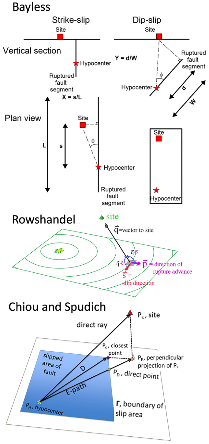
Key model coordinate components for three DMs considered within this article: Bayless, Rowshendel, and the Chiou and Spudich model. Modified from Donahue et al. (2019), Spudich et al. (2014), and Donahue et al. (2019), respectively.

The Rowshandel (2010) DM (as originally detailed in the work by Rowshandel, 2006), referred to as the Rowshandel model throughout the rest of the article, was updated in the work by Rowshandel (2018a) for narrowband characterization and in the work by Rowshandel (2018b) to better capture rupture and slip heterogeneity effects, and most recently to centering. This model is based on the concept that to obtain the maximum directivity effect at a site, the direction of rupture and the direction of slip should both be toward that site. Figure 1 displays the unit vectors used in calculating the dot product of the unit slip and rupture direction vectors that are used to sum up the contribution along the fault. Key differences between this model and others are that it does not classify faults by the style of faulting. Because this approach effectively performs an integral of the slip and rupture over the entire rupture surface, total computation time is substantially increased, compared with other models, even for simple fault sources (but this will vary directly with the discretization resolution chosen along the fault plane).

The Spudich and Chiou (2008) model, highlighted as a chapter in the work by Spudich et al. (2014), is the predecessor to the model referred to as the Chiou and Spudich model going forward. This approach uses the DPP, dependent on the isochrone velocity (Spudich et al., 2004), a measure of rupture propagation distance, and a radiation pattern term. This model was created to remedy flaws in a previous DM that uses the isochrone directivity predictor (IDP) (Spudich et al. 2014). Figure 1 gives an example of the relevant terms needed to compute various factors that go into computing DPP. The calculation of these terms can become quite intensive for complex ruptures that include segments with variations in strike along the fault trace. These model coefficients were originally derived to apply specifically to the CY GMM, but recently have been computed for the other three leading GMMs: BSSA, ASK, and CB (unpublished calculations from Brian Chiou, personal communication, 2022).

Rupture DMs in PSHA

There are various reasons why directivity is not regularly incorporated into hazard studies. Tothong et al. (2007), Spagnuolo et al. (2012), Shahi and Baker (2013), Spagnuolo et al. (2016), and Bayless et al. (2020) outline a wide array of issues. Chief among them is the added computational burden from modeling the hypocenter location, in addition to modeling the fault complexity that exists within source models used in hazard studies, such as in UCERF3 (Field et al., 2014). The directivity adjustments to GMMs depend on a priori knowledge of the hypocenter location, which presents challenges for providing a generalized risk assessment (Donahue et al., 2019; Spudich et al., 2014).

Recently, two groups have made progress toward integrating these various models into a PSHA framework. Al Atik et al. (2023) introduced simplifications to complex faulting systems to implement various DMs (Bayless et al., 2020); the Bayless 2013 model, as summarized in the work by Spudich et al. (2014), and the Chiou and Spudich model, as detailed in the work by Spudich and Chiou (2008). This group was able to successfully compute statewide hazard maps of California including the adjustments for directivity, by smoothing multisegment ruptures and faults with large changes in dip and rake angle within UCERF3 ruptures. Weatherill (2022), and most recently Weatherill and Lilienkamp (2023), also made substantial headway toward incorporating the Bayless et al. (2020) DM into the New Zealand seismic hazard model, assessing the impact of seismic hazard using the Stirling 2012 fault model (Stirling et al. 2012), finding that directivity can influence hazard in the presence of complex faulting systems. As we highlight within the remainder of this article, our work here considers complementary approaches to incorporate directivity into the USGS NSHM, including the capabilities of how DMs can handle complex fault rupture geometries, as well as computational efficiency with respect to adjustments from multiple hypocenter locations.

Several methods are outlined in the literature to incorporate directivity information into seismic hazard models. For example, Donahue et al. (2019) assembled an End-Users Directivity Panel to evaluate the state of DMs with application to the NGA-West2 GMMs and to develop recommendations for future research on near-fault effects. Included within this report were several options to account for directivity within hazard implementations. Out of these possible options, there are two main recommended paths to proceed with adjusting ground motions for amplification predicted from seismic DMs: (1) direct adjustment within the PSHA hazard integral by averaging over multiple hypocenter locations or (2) applying an average median and aleatory adjustment model that a priori has computed the effect of the spatial adjustment to rupture directivity, and thus, the adjustment is added onto ground-motion predictions only once during the hazard calculation for a single source.

The first method considers multiple hypocenter locations throughout the hazard integral, summing over the possible ruptures, and incorporating rupture directivity adjustments in a systematic way by considering all the variations in specific hypocenter and fault geometries. This method captures the epistemic uncertainty in the hypocenter location, necessary for computing fractiles of hazard other than the mean. Although looping over all possible hypocenters for a given fault is the most thorough option, it can be computationally prohibitive for direct integration into PSHA software on a regional scale. To overcome this issue, Watson-Lamprey (2018), hereafter referred to as the WL18, developed a method of adjustment to the median and standard deviation GMM predictions of the CY model (Chiou and Youngs, 2014), to model the effect of multiple hypocenters. This is called the “modification of moment” from randomized hypocenters in the work by Donahue et al. (2019). This method applies a directivity adjustment model to the median and aleatory variability estimates predicted by GMMs, independent of hypocenter. This approach allows the ground-motion adjustment model to be precomputed, prior to the seismic hazard calculation, and is thus a less expensive computational task during the calculation of hazard.

To develop the model, WL18 computed DM predictions and considered multiple hypocenters with varying styles of faulting, magnitude, and distance conditions to develop a database of hypocenter-specific information. The CY model, using the DPP (Chiou and Youngs, 2014), was selected to achieve this. The median and aleatory adjustment terms are computed by summing over the possible hypocenter locations along strike and dip (with a 1-km grid resolution in both strike and dip along the fault surface) and calculating the DPP prediction at that station, with reference to the CY GMM as a function of spectral period. WL18 then found the best-fitting model with respect to the average directivity pattern when considering all hypocenters. We note that this parametric approach approximates the amplification patterns of DPP, but may not resolve all the details when applied to complex fault geometries, a subject we investigate later. Moment magnitudes ranging from Mw 6–8 for strike–slip events and Mw 6–7.5 for reverse events were used to derive the change in the median and standard deviation of the SA due to the randomization of hypocenters along the fault. The complete aleatory variability term includes both the reduction from the average variability over all sites and the site-specific variability due to the source hypocenter distribution. This approach allows for the prediction of a generalized directivity adjustment over a range of magnitudes independent of hypocenter location, for both strike–slip and dip–slip (both reverse and normal) ruptures, permitting straightforward integration into PSHA codes that already predict GMM median and standard deviations. We discuss this method in greater detail in the next section, within the evaluation of seismic DMs within PSHA.

Evaluation of seismic DMs for consideration in PSHA

DM prediction comparison

To make an informed decision about the new considerations that directivity presents for integration into PSHA and the NSHM, we first evaluate the performance of these DMs for simple fault geometries, by comparing input assumptions and output adjustment parameters. Each model requires the definition of the earthquake rupture, including magnitude, fault geometry, rake, dip, and the position of the site relative to the rupture, via fault distance terms. Figure 2 plots the spatial terms of the Bayless, Rowshandel, and Chiou and Spudich model predictions for a hypothetical vertical Mw 7 strike–slip rupture. Figure 2 displays the amplification of response SA at 3.0 s period, but the parameters scale similarly enough with period to generalize the major features. Table 1 highlights the key output parameters of each model. As evident in these spatial plots, some of these terms mimic the SH-wave radiation pattern, thought to be a key contributor to the amplitude of the directivity effect observed in ground-motion records (Somerville et al., 1997). In addition, the total DM adjustments are plotted in natural log units for each model. Here, this spatial adjustment applied to the median GMM prediction has similar characteristics for all three DMs, in terms of distributions of ground motion increases and decreases. However, some models depend on variables that change substantially with more complex ruptures, such as the azimuthal focus and amplitudes of both forward and backward directivity.

Figure 2.

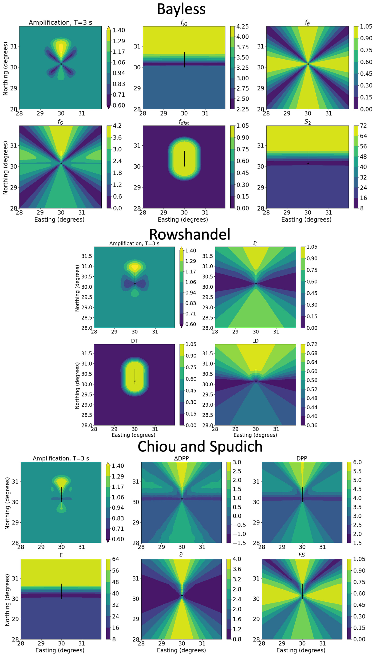
Spatial plots of key terms output from three DMs considered within this work: Bayless, Rowshandel, and the Chiou and Spudich model (all highlighted in the work by Spudich et al., 2014). Table 1 details specifics of the individual terms of each model. These variables combine with unique expressions derived by the developers to create an adjustment to a median spatial amplification factor to apply to GMMs, as shown here in natural log units. Rupture geometry is that of a vertical Mw 7 strike–slip fault of length 80 km, with hypocenter at 8 km depth, indicated by the black star. Plots are shown at a period of 3 s. Units are as specified in Table 1.

Table 1.

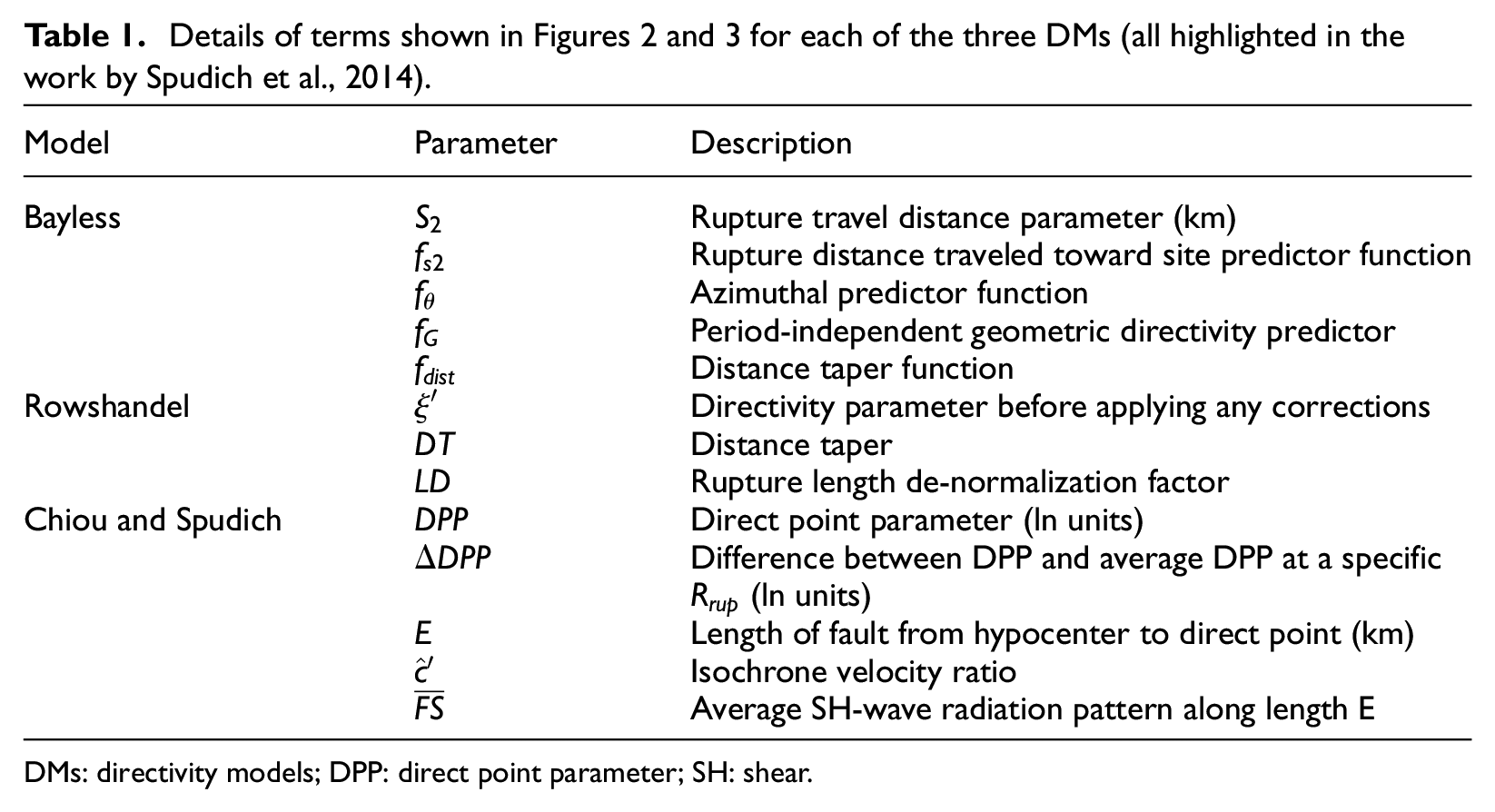
Details of terms shown in Figures 2 and 3 for each of the three DMs (all highlighted in the work by Spudich et al., 2014).

Model	Parameter	Description
Bayless	$S_2$	Rupture travel distance parameter (km)
	$f_{s2}$	Rupture distance traveled toward site predictor function
	$f_{\theta }$	Azimuthal predictor function
	$f_G$	Period-independent geometric directivity predictor
	$f_{\mathrm{dist}}$	Distance taper function
Rowshandel	$\xi \prime$	Directivity parameter before applying any corrections
	$\mathrm{DT}$	Distance taper
	$\mathrm{LD}$	Rupture length de-normalization factor
Chiou and Spudich	$\mathrm{DPP}$	Direct point parameter (ln units)
	$\mathrm{\Delta }\mathrm{DPP}$	Difference between DPP and average DPP at a specific $R_{\mathrm{rup}}$ (ln units)
	$E$	Length of fault from hypocenter to direct point (km)
	$\hat{c}\prime$	Isochrone velocity ratio
	$\overline{\mathrm{FS}}$	Average SH-wave radiation pattern along length E

DMs: directivity models; DPP: direct point parameter; SH: shear.

Previous studies (e.g. Donahue et al., 2019; Spudich et al., 2014) have shown there is substantially less agreement between DMs when evaluated for dip–slip faults. This is compounded by the fact that most DMs do not distinguish upon rake, ignoring whether a dip–slip fault is a normal or reverse rupture within the calculation. To highlight this, we plot spatial adjustment predictions for a dip–slip (normal) fault in Figure 3, with a dip of 60°, keeping all other source terms equivalent to that in Figure 2. This choice emphasizes the deviations in the supplementary terms that lead to the amplification adjustment shown for each DM. There are indeed substantially different patterns among the amplification trends for the three DMs considered here. This information may be utilized in future improvements to DMs, in particular with reference to consideration of the variations in these predictions in both an epistemic framework and possible weighting approach for implementation in PSHA.

Figure 3.

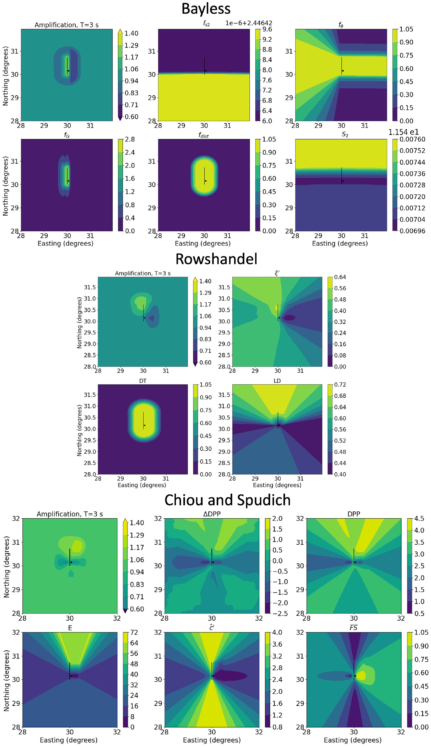
Dip–slip equivalent of Figure 2, showing spatial plots for the same magnitude, length, and width of the fault, but with a dip of 60° (to the right) and rake of −90°, corresponding to values expected from a normal-faulting earthquake. Each DM shown here is highlighted in the work by Spudich et al. (2014).

For some of the DMs, there are parameters that allow variation of the predicted directivity adjustment, specific to characteristics of the event. For example, the description of the Rowshandel model allows specification of the weight on the propagation versus slip contribution to the directivity adjustment within the dot product computation. Here, we use a value of 0.5 that equally weights the contribution of these two terms. Varying this ratio can affect the spatial amplification pattern as shown in Figure 3, but only partly accounts for the differences among the models.

Median and aleatory variability adjustment model

As mentioned previously, there are two main approaches to consider regarding implementation of rupture DMs in PSHA—adjustment within the hazard integral from the contribution of multiple hypocenters, or applying a precomputed adjustment to the median and aleatory variability to account for the cumulative effect of multiple hypocenters. The added computational expense of considering multiple hypocenters is greater than a simple adjustment approach, in particular when computing the required distance terms for the many complex ruptures that exist for sources within UCERF3. WL18 is the only method to date that utilizes the latter approach. Figure 4 gives examples of the spatial adjustment pattern resulting from directivity predicted by this model for both strike–slip and normal-faulting scenarios. The cumulative effect of multiple hypocenters for this scenario strike–slip fault with constant strike produces symmetric lobes of increased median amplitude off the ends of the fault, with regions of smaller values along the fault trace, consistent with centered results from the DPP model predictions (as gleaned from Figure 2). The corresponding standard deviations have a “butterfly” pattern at this chosen Mw, with two regions of larger values off the end of the fault but with minimal changes along strike.

Figure 4.

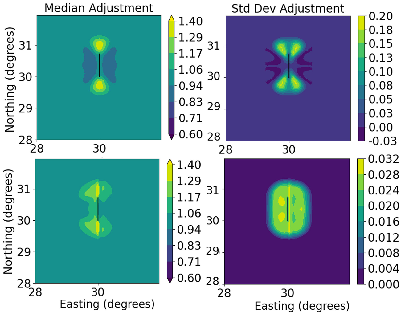
Spatial patterns of the predicted adjustments of natural log mean and aleatory variability (resulting from the randomization of hypocenters) at 3 s SA using WL18’s “preferred” model (referring to the hypocenter distribution) for a Mw 7 strike–slip (top row) and dip–slip (bottom row) fault, corresponding to the rupture geometry as shown in Figures 2 and 3.

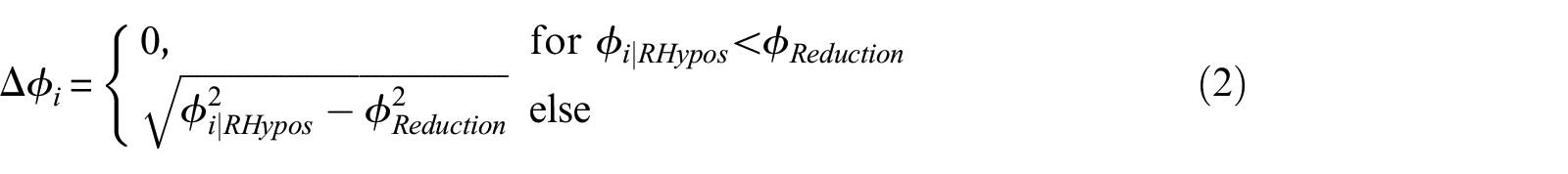
These aleatory variability terms plotted in Figure 4 only include the effect of considering multiple hypocenters. The change in the published GMM aleatory variability due to the effects of directivity has two components. The first component, a reduction, is the decrease in variability due to improvements in the median prediction—this is the reduction in variability caused by including the directivity term in the GMM regression. The second component, an increase, is the variability of the change in the median at a given site due to directivity from all sources and hypocenters. In practice, there is not consensus on how to treat these components nor the appropriate values for each of them. The WL18 method defines the change in aleatory variability to be an increase only (but may deviate slightly from this constraint due to the model’s ability to fit the data); if the reduction term is larger than the increase due to randomized hypocenters, the net change in variability is set to zero. In this study, we compute the total standard deviation by computing the differences in the variances listed above as:

$${\varphi }^2={\varphi }_{\mathrm{GMM}}^2-{\varphi }_{\mathrm{Reduction}}^2+{\varphi }_{\mathrm{RHypos}}^2$$

(1)

in combination with WL18 Equation 1.7:

$$\mathrm{\Delta }{\varphi }_i=\{\begin{array}{c}0,\mathrm{for}{\varphi }_{i|\mathrm{RHypos}}<{\varphi }_{\mathrm{Reduction}}\hfill \\ \multicolumn{1}{c}{\sqrt{{\varphi }_{i|\mathrm{RHypos}}^2-{\varphi }_{\mathrm{Reduction}}^2}\mathrm{else}}\end{array}$$

(2)

where ${\varphi }_{\mathrm{RHypos}}^2$ is the associated variance from randomized hypocenter locations; ${\varphi }_{\mathrm{Reduction}}^2$ is the variance reduction term; and ${\varphi }_{\mathrm{GMM}}^2$ is the reference is the original, adjusted variance of the GMM. We consider some of the potential implications of this assumption in the “Discussion” section.

The dip–slip prediction in Figure 4 displays a positive median adjustment located on the footwall side of the fault, with a negative region along the fault trace. The standard deviation is positive, but it has a substantially reduced amplitude compared with the strike–slip model. This aleatory variability here varies with period in the model, dependent on the change in the mean that has a peak directivity effect that varies with magnitude. We note that we have only been able to validate strike–slip models when comparing to figures in the work by Watson-Lamprey (2018), observing slight discrepancies between dip–slip models at distances close to the fault. This may be due to incorrect assumptions about the input fault parameters (some of which are not clearly specified within the report) or a possible error within the tabulated coefficients listed within the model. We take this into consideration when determining PSHA integration options later within this article.

Rupture DM adjustments to GMMs

We previously analyzed baseline adjustments to several DM predictions. It is enlightening to view the influence of directivity on the overall level of ground motion by adding directivity adjustments to GMM predictions. Figure 5 plots the spatial prediction of SA at a period of 3 s for the average of four GMMs (BSSA, ASK, CB, and CY) for a subsection of the San Andreas Fault with a magnitude Mw 7.2. The plots in the second column of Figure 5 show the spatial amplitude prediction of forward and backward directivity for this fault rupture and the hypocenter for the two relevant DMs considered here. The WL18 plot is singled out on the bottom row here, as it is distinct from the other two models, representing an average over all hypocenters (and illustrates the effect of the Chiou and Spudich DM). It is informative to compare the spatial prediction of the WL18 model for a fault rupture that has variations of rupture geometry along strike with DMs that are hypocenter dependent. We observe that even with the variation in fault geometry, both the hypocenter-dependent and WL18 model modifications to ground motion are generally symmetric about the fault plane, with increases off the ends of the fault and a smaller negative adjustment along strike. The third column in Figure 5 shows the superposition of the directivity adjustment and the GMM predicted average. We note that some of these DMs were derived with specific GMMs in mind, but due to the similarity between the ground-motion predictions, we do not notice a substantial difference in behavior when applying them to additional GMMs. These effects vary in magnitude among the three models, but generally, the models have similar characteristics. As expected, the main effect is to increase the level of ground motion in lobes off the ends of the fault, elongating the ground-motion amplification pattern, with a minor reduction in amplitude along the fault trace. In the last column, we also plot the aleatory variability for the Bayless and WL18 models that include a standard deviation adjustment. The Bayless aleatory model is strictly a reduction term, whereas the WL18 model includes both the decrease in standard deviation from fitting the ground-motion distribution better due to modeling directivity effects and the implicit increase from hypocenter randomization. The overall effect is an increase in standard deviation added to the ground-motion variability, which, as we will point out later, can potentially affect hazard.

Figure 5.

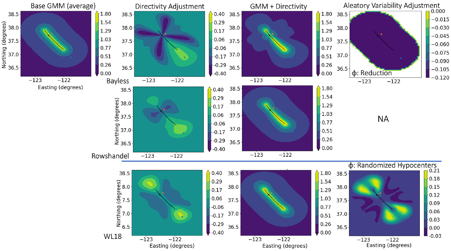
Spatial adjustments from several DMs (each DM shown here is highlighted in the work by Spudich et al., 2014) compared with the base GMM prediction SA (m/s²), first column), plotted both individually (second column), and added on to the average of the GMM predictions (third column) at a period of 3 s for a fault with a magnitude of Mw 7.2. In addition, aleatory variability is shown for models that include a spatial standard deviation adjustment (for the Bayless model this is a reduction term, while for WL18 model this is the combination of the reduction term and the increase resulting from the effect of randomization in hypocenters, the latter of which is plotted here). Triangles indicate station locations analyzed in Figure 6. We highlight WL18’s hypocenter-independent model separately, as it incorporates an average over multiple hypocenter locations, as opposed to being hypocenter-specific (but hypocenter symbol is still shown for comparison with above plots). Site conditions are held constant throughout the model, with a $V_{s30}$ (the time-averaged value of the SH-wave velocity in the top 30 m) of 760 m/s.

To investigate the ground-motion adjustment comparison further, we highlight two example stations, analyzing sites in both the forward and backward directivity directions. Figure 6 shows the trends of these two selected stations with period, and how the corresponding levels of adjustment vary when added onto GMMs. It is clear that both positive and negative variations in the ground-motion amplitude can be achieved from the effects of a directivity spatial adjustment model. The WL18 model includes the averaged effect of all hypocenters, so it is not a direct comparison with the other two models but serves as helpful insight into the level of variation among the models.

Figure 6.

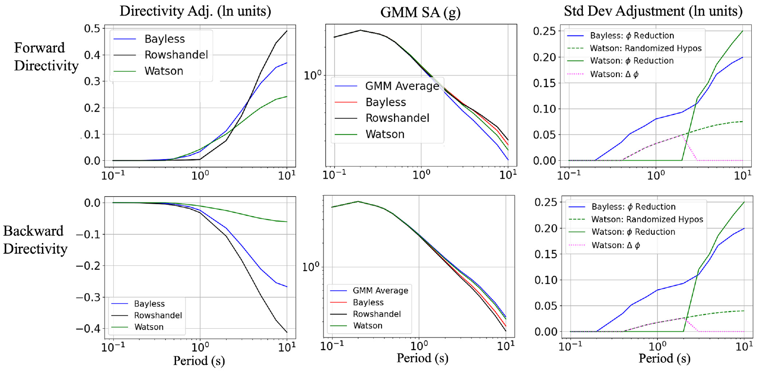
Example comparisons of forward and backward directivity for the two stations in Figure 5 that lie in the forward and backward directivity directions. We plot the logarithmic directivity adjustment separately (left column), highlighting the difference in amplitude between the models, as well as the superimposed effect on the GMM prediction (center column). For models that include a standard deviation adjustment, we plot the natural log prediction as a function of period (right column). The Bayless and Rowshandel DMs are highlighted in the work by Spudich et al. (2014), while the WL18 DM is detailed in the work by Watson-Lamprey (2018). SA: spectral acceleration.

The standard deviation adjustments are shown for reference here, which includes the various terms in Equations 1 and 2. This includes the increase from the effect of hypocenter randomization for the WL18 model. Although these terms are from different models, the relative amplitude between these two aleatory variability components is important in determining which term is more important within the hazard calculation, a concept considered within the “Discussion” section.

Application in seismic hazard analysis

To account for directivity effects in hazard evaluation, we first implemented the WL18 approach, which adjusts the median and aleatory variability of the GMM, as it is the most practical method to proceed with integration into current USGS PSHA software. Guided by the agreement among the DMs considered here for strike–slip ruptures and supported by previous studies (e.g. Donahue et al., 2019), we limit our initial implementation to strike–slip faults. Excluding directivity adjustments from dip–slip faults minimizes the potential discrepancies that may arise from choosing a single model that may not capture the epistemic uncertainty that exists when considering multiple DMs. This is a first step toward gauging the importance of the effect of directivity on seismic hazard. In addition, this approach established a means to work through some of the issues that need to be addressed when considering the added complexity of modeling the effects of hypocenter location in hazard calculations. The alternative, to incorporate an additional integral over the hypocenter location, was less practical at this point for regional considerations with a substantial number of fault ruptures, such as in UCERF3 (Field et al., 2014), as calculation of the additional distance terms needed is computationally intensive, and added another layer of calculations to the problem. In the following subsections, we describe the implementation of WL18’s “preferred model” in the USGS hazard software, nshmp-haz (Powers et al., 2022), using the version derived with a hypocenter distribution probability that varies along both strike and dip.

Coordinate system and distance term computation

To implement WL18 into the nshmp-haz code, a coordinate system to define site-to-source distance terms for both simple and complex faulting systems is needed. Because of its proficiency in handling discontinuous segments, we chose the GC2 system (Spudich and Chiou, 2015) that integrates near-source fault trace information to produce a consistent representation of fault-parallel and fault-perpendicular distance metrics. This method provides fault distance terms for complex fault geometries and is a prerequisite for several DMs, including the technique of incorporating the median and aleatory adjustment model with complex fault models, as used here. The first step toward incorporating the WL18’s model into the nshmp-haz code was to add the GC2 calculation into the code to compute $R_x$ and $R_y$ , the strike-normal and strike-perpendicular component distance terms, respectively. These are effectively the T and U coordinates computed in GC2, ignoring a shift in $R_y$ due to the hypocenter location along strike. Figure 7 plots the key distance terms computed for a hypothetical vertical strike–slip fault with strike at 90°, including $\mathrm{T}(=R_x)$ , U, and $R_y$ . We also illustrate the distance terms for a more complex faulting system, a realization of the Calaveras fault, extracted from the UCERF3 model, composed of 27 subfaults along 3 fault sections. Contours of the distance terms demonstrate that the sinuous variations in strike translate out to distance in the $R_x$ term, remaining parallel to the closest point perpendicular to the rupture. As these distance terms are only needed for sites close to the rupture (the region of influence for the Watson–Lamprey model only extends to 70 km $R_{\mathrm{rup}}$ ), we exclude the calculations for stations farther from the fault in the hazard code, and thus are not plotted here.

Figure 7.

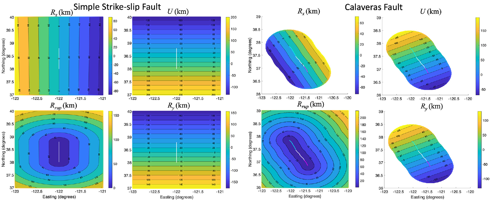
Plots of fault distance coordinates, including GC2 values ( $U$ and $T$ ) for a simple strike–slip fault (left) and for the more complex Calaveras fault (right). Contours of each parameter are shown, with a 70 km $R_{\mathrm{rup}}$ cutoff for terms relating to fault-parallel and fault-perpendicular coordinates for the Calaveras fault, as the predicted directivity adjustment is zero at these distances using the WL18 model (Watson-Lamprey, 2018). Note that the only difference between $U$ and $R_y$ is a lateral shift in the coordinates along strike.

Seismic hazard analysis and sensitivity

As a first step toward integration into the USGS NSHM, we analyze the behavior of the WL18 model for simple fault geometries to develop a sense of the effect of directivity on hazard, without additional complexity. Figure 8 shows a hypothetical Mw 7.0 strike–slip rupture with a return period of 100 years. We plot the total mean hazard for 2%, 5%, and 10% in 50-year probability of exceedance (PoE) for models with and without the WL18 adjustment, for the average of the four GMMs considered here. For simplicity, we use a uniform $V_{S30}$ (the time-averaged value of the SH-wave velocity in the top 30 m) of 760 m/s and ignore basin effects in all of our subsequent analyses to focus on the relative importance of directivity for various rupture realizations. It is difficult to observe substantial changes in the amplitudes by analyzing absolute level of ground motion plotted in Figure 8, but it is evident that the hazard does increase at the ends of the fault and narrows the regions along strike toward lower values. This is expected, given the spatial patterns of plots in Figure 4, but here the effect on hazard is the combined response from both the median adjustment in combination with the change in standard deviation.

Figure 8.

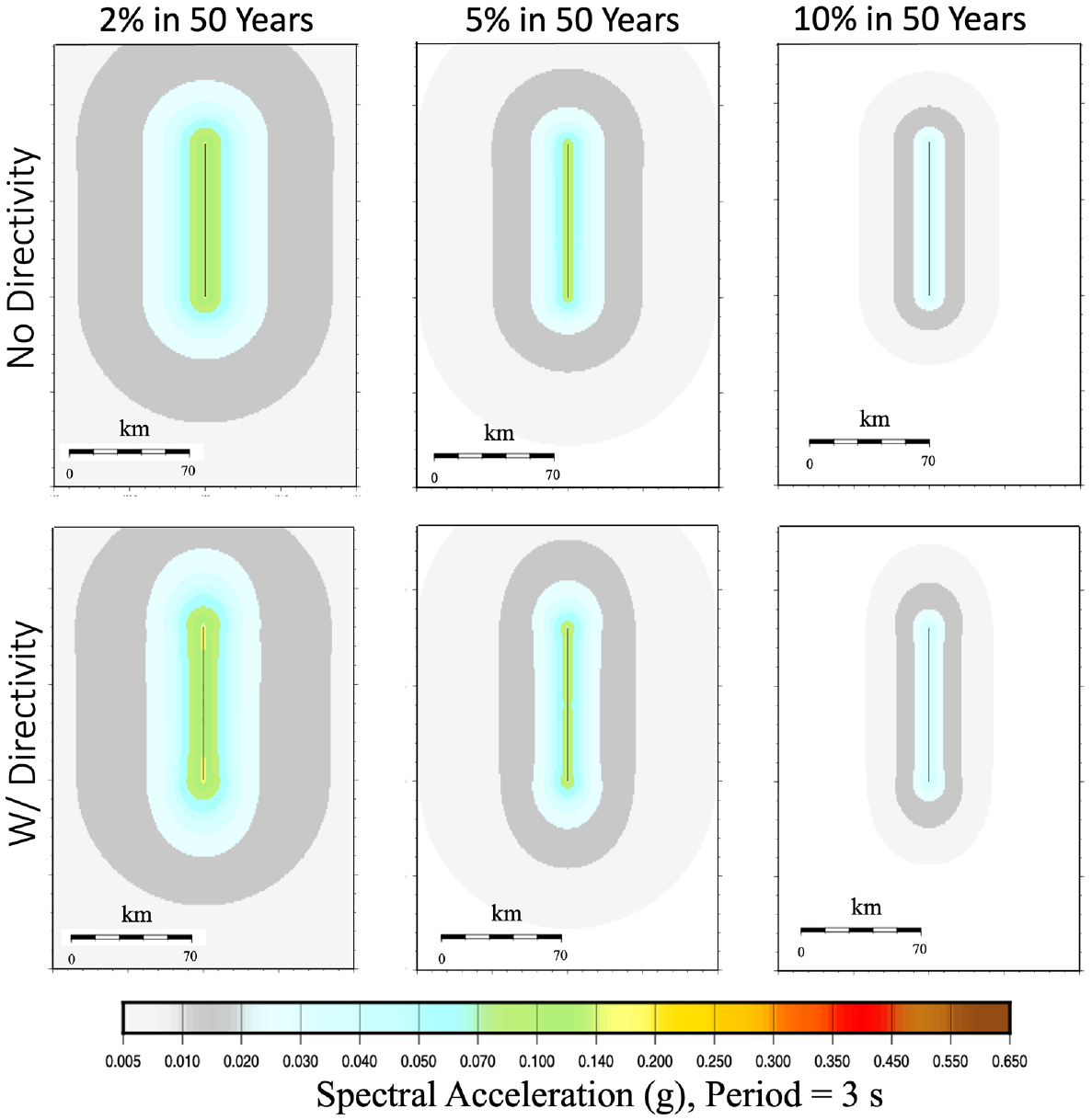
Ground motions plotted for probability of exceedance of 2%, 5%, and 10% in 50 years for hazard models without (top row) and with (bottom row) the WL18 (Watson-Lamprey, 2018) directivity adjustment using the four NGA-West2 GMMs defined in the main text for a period of 3 s. The fault is a hypothetical Mw 7 strike–slip model, with geographic scale for reference—we chose to test implementation of our adjustment method with a simple fault to help verify implementation accuracy and to develop a sense of the effect of directivity on hazard. The slip rate here is set to a constant, with a characteristic magnitude of Mw 7 and recurrence rate of 0.01.

An easier way to visualize the importance of the effect of the directivity on hazard from Figure 8 is to plot difference and ratio maps with and without directivity included within the hazard calculation. Figure 9 plots these for 2% and 10% PoE, emphasizing the characteristic patterns displayed in Figure 8, where the increase in hazard is oriented off the ends of the fault. The scale bars are left at their default level here, showing variations up to 0.06 g (acceleration due to gravity) for this figure, to emphasize that these changes are fairly minor when comparing the absolute difference between the models for a single strike–slip rupture. The maximum percentage change is mainly constrained to within a 20%–30% increase in the lobes at the ends of the fault, with a smaller change of 10%–15% decrease along strike, due to the centered nature (azimuthally around the fault) of the DPP distribution that the WL18 model is based upon. As expected, we observe smaller differences at 10% PoE in 50 years here because of the influence of the aleatory variability, which drives the slope of the hazard curves and is more impactful at long return periods. However, as shown in Figure 6, the effect of aleatory variability is reduced at longer periods, where the cumulative effect of both terms is minimal.

Figure 9.

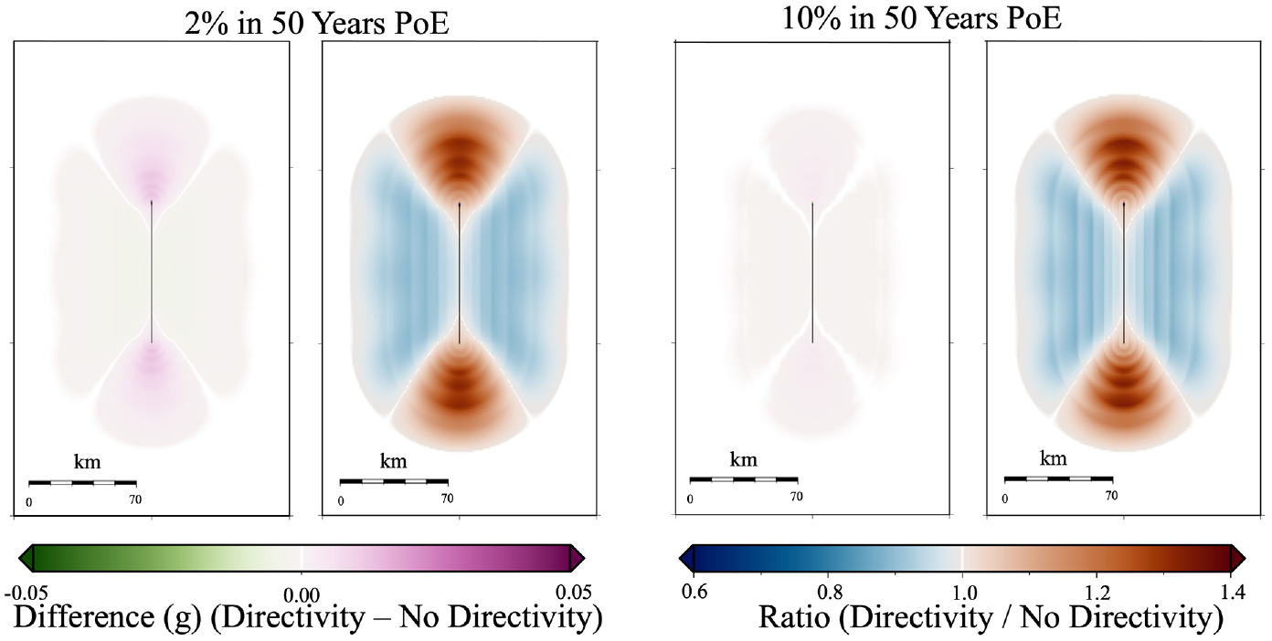
Difference and ratio plots of hazard at the 2% and 10% levels of probability of exceedance in 50 years for a period of 3 s, derived from the plots as shown in Figure 8, highlighting the spatial variations due to directivity adjustments from the WL18 model (Watson-Lamprey, 2018).

This first example showed the directivity influence on hazard from a single rupture, highlighting that the amplification can reach an amplitude of up to 30% to 40% off the end of the faults, with a broad region of decreased ground motion parallel to the fault plane. These spatial patterns will be altered, however, when the cumulative effect of multiple fault sources is introduced, where the individual adjustments superimpose at stations near the fault. To test the effect from multiple sources, we computed hazard for successively more complex fault models. An example is shown in Figure 10, for a series of one to three hypothetical strike–slip faults, offset both parallel and perpendicular along strike (each with the same rate). The cumulative effect shows that positive and negative regions serve to destructively interfere along the fault trace, reducing the absolute amplitude of the directivity effect. The selected faults here still have a tendency to amplify the regions off the ends of the ruptures but vary with the specific locations and geometry of the fault traces. We further examine the implications of the potential effect of source geometry within the “Discussion” section.

Figure 10.

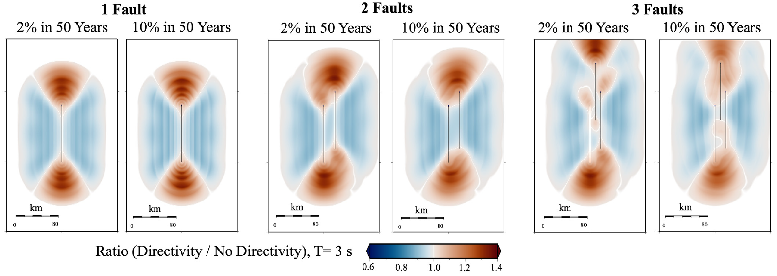
Example of the effect of the superposition of directivity adjustments from multiple sources on hazard, for a series of hypothetical strike–slip faults, offset both parallel and perpendicular along strike (distance scale provided for reference) at a period of 3 s. These plots use the four NGA-West2 GMMs and same magnitude and recurrence rate as shown in Figure 8.

The WL18 model was not derived from irregular shaped or discontinuous ruptures, and thus, there is the possibility that model predictions may not extend accurately to complex ruptures, such as those that exist within UCERF3. Thus, to evaluate whether WL18’s expressions remain reasonable for these rupture geometries, we compare iteratively more complex models. Figure 11 plots difference and ratio plots (with and without including directivity) for a single rupture along the Calaveras fault model (as shown in Figure 7). Even with the additional fault complexity here, the WL18 model appears to capture the main features present in simpler strike–slip models, not greatly influenced by variations in sinuous geometry along the fault trace. For example, as in the simple strike–slip plot in Figure 9, lobes of larger values are present off the ends of the fault, with larger amplitudes at lower probabilities of exceedance. These results indicate that even though the WL18 model was not derived using complex fault geometries, its dependence on the fault-parallel and fault-perpendicular terms via GC2 gives it the ability to match the characteristics needed for practical computation of the spatial directivity characteristics for more intricate rupture geometries.

Figure 11.

Similar format to Figure 9, displaying ratio and difference plots at a period of 3 s from a rupture along the Calaveras fault model, extracted from the UCERF3.1 source model (Field et al., 2014). “PoE” is abbreviation of probability of exceedance.

In the course of evaluating the effect of directivity on these simple fault model geometries, we have found that in applying WL18’s model to complex faults, averaging the weighted input parameters (such as the choice of dip across a multisegment fault) can affect the spatial pattern of directivity adjustment. We hypothesize that the potential bias associated with using an averaged value to compete these predictor variables, as is necessary for the WL18 model and many other DMs, can impart a greater effect on the results on the near-source directivity prediction for complex fault systems than the potential inaccuracies present here from using a hypocenter-independent model not derived using complex fault geometry. We leave the consideration and evaluation of the best scaling relationships to apply to subfaults with varying geometry conditions that contribute to the input parameters of DMs for future work.

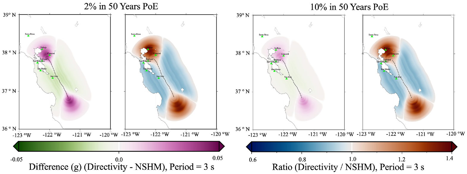
To continue illustrating the implementation of directivity adjustment for progressively more complex fault geometries, we next analyze the full-scale fault model in the NSHM. We continue to use California as a testing platform to assess the effect of directivity on hazard. Figure 12 plots difference and ratio maps that include ruptures from the UCERF3 fault model (Field et al., 2014). Because of the variability among DM predictions observed in dip–slip faults, we limit directivity adjustments to only strike–slip faults here, defined as the average dip (computed as area-weight averaged) being greater than 75°. This restriction only reduces the number of fault ruptures by approximately 10% in the region considered. The resolution of the plots in Figure 12 is limited here, due to the restriction on the number of stations where hazard is computed—as mentioned previously, incorporating the additional GC2 distance terms increases the computational time within the hazard calculation, scaling linearly with the number of fault ruptures considered. With approximately a quarter million possible ruptures potentially contributing to hazard within this region (many of the ruptures are large in magnitude and thus length, having a wide region of influence), we chose a grid size of 0.1°, in order for the hazard calculation to complete in a reasonable amount of time on our local machine (the computational effort here is mainly due to the computation GC2 distance terms, not the directivity adjustments). Analyzing the resulting difference and ratio plots, we observe that the bulk of the region has an adjustment within $5$ % of the model without directivity. The reduced effect, compared with the adjustment from a deterministic scenario, is expected from the visualization of the iteratively more complex fault distribution as shown in Figure 10. As more and more faults align near one another and exist along strike, the more opportunity for destructive interference to limit the peak amplification that may occur for a single event. There will still likely be places toward the edge of these source models, however, where the spatial superposition from multiple faults does not occur as readily.

Figure 12.

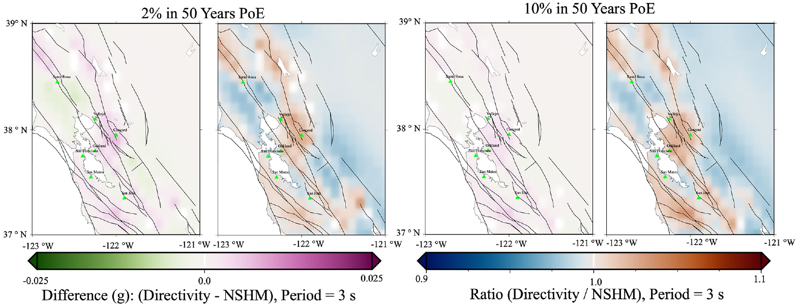
Similar format to Figures 9 and 11, but including the entire UCERF3.1 (Field et al., 2014) fault model (excluding dip–slip faults), displaying hazard differences and ratios in the San Fransisco Bay region with and without including directivity for a period of 3 s applied to the four NGA-West2 GMMs. Green triangles indicate locations of major cities and selection of stations, some of which are compared in Figures 13 and 14. “PoE” is abbreviation of probability of exceedance.

To investigate the effect of directivity more closely, we evaluated hazard at several stations as a function of period. Figure 13 plots hazard curves for three locations with and without directivity against the corresponding annual frequency of exceedance at several periods (1, 3, and 5 s). The addition of directivity affects the hazard at each of these stations, varying with amplitude as a function of period. The directivity influence is minimal at a period of 1 s, but increases to larger amplitudes at periods of 3 and 5 s. This is expected from the narrowband nature of the DM adjustments, scaling with magnitude and period. The shape of these hazard curves slightly elongates (flattens) from the effect of the change in sigma, typically decreasing in slope when including directivity effects, which will likely affect disaggregation results computed for these stations.

Figure 13.

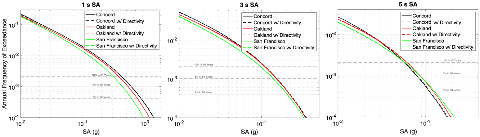
The annual frequency of exceedance at several stations extracted from Figure 12, with and without directivity at three periods, to help gauge the period dependence of the directivity adjustment at locations of interest. Solid lines indicate the models without a directivity adjustment while the dashed lines include the adjustment from the WL18 model (Watson-Lamprey, 2018). The 2%, 5%, and 10% levels of exceedance in 50 years are shown for reference.

We also compute uniform hazard spectra for these three stations. Figure 14 plots the ratios with and without directivity, indicating that most of the directivity influence is present at periods greater than 1 s. The ratios here generally lie within 1%–2% in this period range. The ratios reflect the combined influence of the median and standard deviation adjustment with the variation in period, combining to form a net positive adjustment for two of the three stations shown here. The contribution derives mostly from the median adjustment—the influence from the standard deviation adjustment component is minimal, as the change in the aleatory variability is close to zero when accounting for both the increase from randomized hypocenter locations and the reduction from better fitting the ground motions. This is true particularly at longer periods, when the reduction term becomes larger than the increase in aleatory variability from randomized hypocenters, where the total adjustment in WL18 is defined to be zero.

Figure 14.

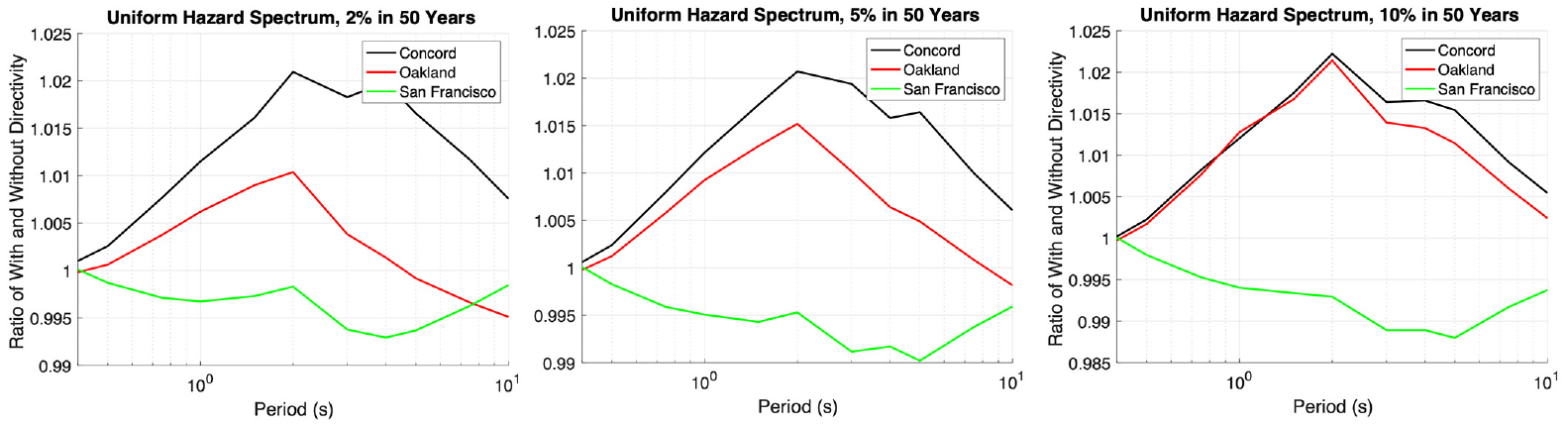
Ratios (with directivity/no directivity) of uniform hazard spectra at 2%, 5%, and 10% in 50 years for stations plotted in Figure 13, displaying the variation of directivity adjustment with period. SA: spectral acceleration.

These previous figures outlined how directivity can affect seismic hazard, focusing on the regional scale. Again, because of the sheer number of ruptures contained within UCERF3, including directivity adjustments in California statewide hazard maps substantially increases the computation time, due to the added complexity of computing GC2 distance terms when considering all the possible fault ruptures that may contribute to a specific site. We select one period to analyze the statewide hazard map of California arising from the UCERF3 model (still constrained to strike–slip faults) in Figure 15. The statewide maps show similar levels of adjustment, compared with the regional map as shown in Figure 12, typically within 5%–10% of the reference model without directivity, but there are regions of larger amplification off the end of fault ruptures, as well as where ruptures are constrained geometrically within the source model. For example, the large increase in central California likely comes from the creeping section of the San Andreas Fault off the southern end of the Calaveras fault, for which ruptures in UCERF3 are less likely to pass through. Effects arising from the specified source geometry warrant being analyzed in the future to determine the significance of these boundaries that influence ground-motion amplification from directivity.

Figure 15.

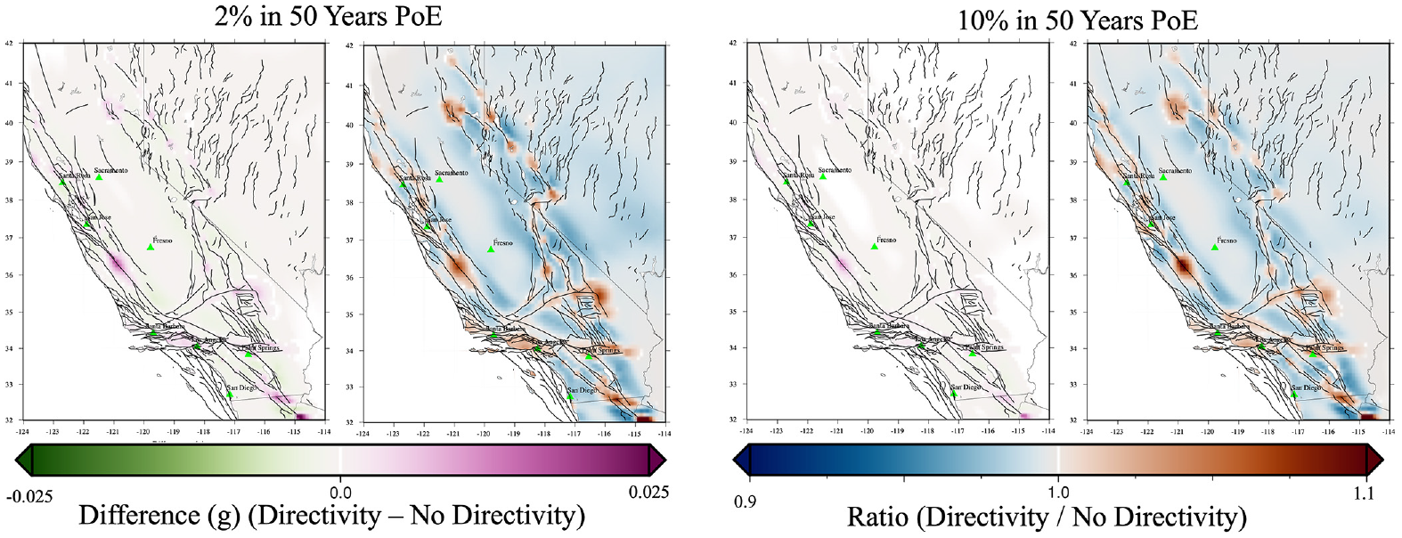
Difference and ratio plots of statewide hazard maps including California and Nevada, including strike–slip ruptures from the conterminous US model, at the 2% and 10% in 50-year levels of probability of exceedance for a period of 3 s.

Discussion

A substantial amount of detail within the DMs and implementation specifics has been glossed over within the main text of this article. We go into greater detail here for several subjects that warrant discussion and further investigation within future studies, to better assess the significance of derivation assumptions, implementation consequences, and the future accuracy of hazard computations.

Rupture directivity adjustment models

There are several assumptions made here to successfully implement a rupture directivity adjustment model into a modern PSHA software. A key among these is the ramifications of using a model of a model, as we have performed when choosing the WL18 DM as our directivity adjustment method of choice here. In effect, we are relying on the WL18 model’s ability to capture the behavior of Chiou and Young’s DM, and thus, results will be subject to assumptions and interpretations made within that model’s formulation.

The WL18 model was a substantial initial step toward making directivity calculations practical in a PSHA framework. However, there are improvements that can be made to better match the DM behavior it is based upon. For example, in the Pacific Earthquake Engineering Research (PEER) report (Watson-Lamprey, 2018), as illustrated in several plots therein, there are substantial differences between data and the model predictions, in terms of overall trends with azimuth, as well as deviations in the amplitude of the model predictions. Thus, future improvements may modify the behavior of some of the model predictions presented here. Nevertheless, the existing implementation provides a useful comparison for an assessment to evaluate differences going forward. Our efforts have focused on implementation of a single preexisting model. In the future, efforts toward expanding to other methods using simplified directivity adjustment models, such as additional seismic DMs, may allow better assessment of epistemic uncertainty when implemented into the NSHM and ultimately a better assessment of seismic hazard.

An alternative approach may better fit residuals to median and standard deviation adjustments. Possible routes to pursue include nonparametric methods to better fit the non-Gaussian shape of the DPP distribution, or machine learning approaches, using a larger set of training data. For example, Kelly et al. (2022) recently initiated an approach to developing a correction-type method (independent of hypocenter) using a neural network method that interpolates across a range of source characteristics, including fault dip, strike, and magnitude using synthetically generated data from the Chiou and Spudich DM. Adjustment factors are precomputed for varying styles of faulting, magnitude, and distance conditions to develop a database of hypocenter-specific information. These preliminary results have shown this to be an accurate method to match the underlying DM characteristics.

Directivity from subset of UCERF3 source model

We computed the hazard for the entire state of California (constrained to strike–slip faults) in Figure 15. Because of the numerous variations in fault geometry within UCERF3, this is an expensive computational calculation. As changes in the underlying hazard model are enacted in the future, it may be beneficial to forgo the full-scale fault model computation, to establish a quicker turnaround time from hazard calculations related to directivity. Motivated by this computational constraint, we tested an approach that encapsulates the highest slip-rate strike–slip ruptures, primarily the six “A” faults outlined in UCERF2 (Field et al., 2009). This consists of the Hayward/Rodgers Creek fault zone, the San Andreas Fault (encompassing both the north and south sections), and the San Jacinto, Elsinore, Calaveras, and Garlock faults. These faults are constrained to dips $>75$ ° and rakes corresponding to strike–slip faults, fitting within the confines we have initially chosen to restrict directivity adjustments to. We performed an inversion using OpenSHA tools (Field et al., 2003) that computes the corresponding slip rates along these six “A” ruptures using the statewide distribution of strain rates. This approach ensures that the ruptures have self-consistent slip rates with a smaller selection of ruptures.

We performed calculations using this selection of ruptures for a statewide hazard assessment with and without rupture directivity. Figure 16 plots difference and ratio plots of the 2% and 10% PoE at a period of 3 s for models that include these individual ruptures. Similar to the regionally focused plots, the hazard is generally modified less when considering directivity along the main sections of the fault planes, following the 70-km region of influence from the faults. The regions of more substantial changes in hazard are located in regions of fault geometries that don’t include as much variation in rupture complexity, where the positive amplification from the directivity prediction spatially dominates off the ends of the fault. Comparing the full fault complexity from UCERF3 in Figure 15, to the selection of faults used in Figure 16, we notice that many of the same regions of amplification are present between the two models, indicating that there does remain some consistency in the expected directivity adjustment resulting from the choice of source selection. One observed difference is the creeping section region that is strongly amplified in the full UCERF3 fault geometry now plays a comparably smaller role with less destructive interference elsewhere along the fault. Note the increased range in the color bar scale of Figure 16—the regions here are larger in amplitude than those present with more complex faults, as in the full UCERF3 source geometry. This may be indicative of the relationships that may exist when directivity is expanded to regions across the conterminous United States, where there is generally less fault complexity, which tends to result in reduced amplifications.

Figure 16.

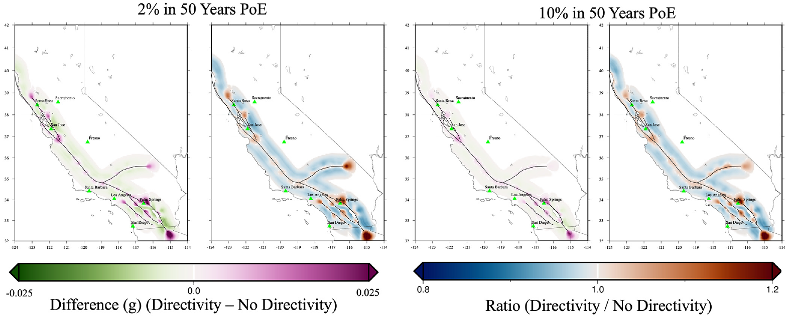
Difference and ratio plots of 2% and 10% in 50-year probability of exceedance mean hazard adjustments for the state of California using six “A” faults, selected as the six key faults with the highest slip rates that contribute most to hazard within the state of California for a period of 3 s.

Methods to improve computational efficiency in hazard calculations

The leading motivation for focusing hazard calculations on a reduced subset of faults is that it is computationally burdensome to compute full-scale hazard maps of California using the entire UCERF3 set of fault ruptures. This is a substantially increased PSHA computation now with the added complexity of calculating GC2 distance coordinates, making it somewhat prohibitive to compute hazard maps including these modifications in the underlying calculation. Utilizing the reduced number of calculations can make it easier to more quickly assess the importance of a change in these initial conditions.

There are several possibilities to improve upon the efficiency of the implementation of directivity and GC2 calculation within the nshmp-haz code (Powers et al., 2022). As currently implemented, there are many redundant calculations when computing distance terms on a site-by-site basis. A more efficient method may be to precompute GC2 distance terms by looping over sites that lie near the same collection of faults, grouping the calculations to avoid repetitive calculations for nearby stations. Alternatively, an initial loop over all fault sources to calculate GC2 distance terms before performing the loop over stations may be practical as well, if the fault information can be stored in memory. These approaches would need to be further evaluated as PSHA studies are scaled to high-performance computing or other massively parallel computational infrastructures moving forward, to determine the most efficient method to account for the effect of directivity.

If the advancements mentioned above prove still too computationally expensive for practical NSHM calculations, there are other techniques that could be pursued to offset the computational burden of computing directivity effects when computing the statewide hazard assessment. One method we propose is to precompute hazard adjustments for a gridded map, accounting for the relevant faults of interest that could be added onto hazard assessments without directivity. There are details to work through here to ensure these adjustments are used in a consistent manner (because there may not be a linear relationship between hazard adjustments), but it is likely sufficient accuracy could be obtained by applying a scaling factor to represent the bulk effect of directivity in regions where it is difficult to compute directivity on the fly. In the end, however, there may not be a universally optimum strategy of directivity implementation in hazard; the most appropriate method may depend on the specific target, whether it be regional scale maps or site-specific analysis for structural design.

Rupture DM guidelines

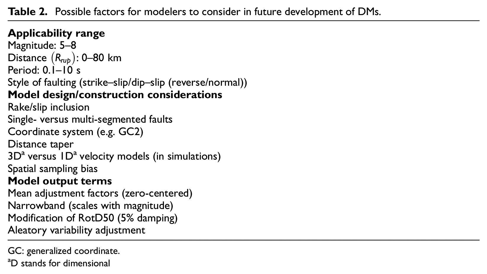
Motivated by the recent USGS update that established minimum requirements and guidelines for acceptance of GMMs (Rezaeian et al., 2021), we propose to establish criteria for acceptance of DMs moving forward. As it is difficult to set the same stringent guidelines as set forth within GMMs, we do not suggest an exact emulation of this procedure for DMs. This is partially because there are far fewer DMs to consider, and thus removing just a single model may substantially affect epistemic uncertainty. In addition, each developer has their own method and approach to adjusting ground motion for directivity effects.

In an effort to simplify the implementation for future PSHA applications, we suggest DMs be evaluated in a similar fashion to GMMs. We outline three main categories: (1) applicable range, (2) model design (including construction issues to consider), and (3) model output terms. We briefly describe criteria for each of these topics, with specific concepts to consider within each group, tabulated in Table 2. First, the models would need to have a minimum region of applicability to ensure there is common ground when computing directivity effects to adjust ground motions. We propose a minimum applicability range of earthquake magnitude ranging from 5–8, rupture distance from 0–80 km, spectral periods of 0.1–10 s, and strike–slip or dip–slip faults (the latter potentially broken up into reverse and normal styles of faulting if preferred). Most DMs already encompass this range, but new taper definitions or parameter extensions may be necessary to include for some models. For example, as more DMs are incorporated into hazard calculations, dip–slip faults likely would need to be considered more consistently. Currently, a normal versus reverse fault distinction is not considered in most of these models (except for the Rowshandel DM, which implicitly incorporates variation in style of faulting via the use of rake).

Table 2.

Possible factors for modelers to consider in future development of DMs.

Applicability range

Magnitude: 5–8

Distance $\left(R_{\mathrm{rup}}\right)$ : 0–80 km

Period: 0.1–10 s

Style of faulting (strike–slip/dip–slip (reverse/normal))

Model design/construction considerations

Rake/slip inclusion

Single- versus multi-segmented faults

Coordinate system (e.g. GC2)

Distance taper

3D a versus 1D a velocity models (in simulations)

Spatial sampling bias

Model output terms

Mean adjustment factors (zero-centered)

Narrowband (scales with magnitude)

Modification of RotD50 (5% damping)

Aleatory variability adjustment

GC: generalized coordinate.

a

D stands for dimensional

Within the model design category, we include consideration of the functional form of the DM and how the models will be implemented. Table 2 lists features to consider as DMs are developed, which will help add consistency to integrations of PSHA across multiple models. We propose DMs that utilize a GC system approach (the GC2 coordinate system in particular), which enables consistent calculation of distance terms and is able to handle complex fault geometries, critical for accurate computation of directivity adjustments at near-source distances. We propose the future DM developments to consider the GC2 approach to enable implementation and evaluation of DMs within PSHA going forward. Some of the development considerations in Table 2 may lead to improved characterization of ground-motion amplification. For example, simulations have been used to illuminate directivity characteristics along both strike–slip and dip–slip events, and serve as a resource to help fine-tune distance relationships and other behavior that has sparse data resolution at near-source distances. Simulation efforts likely would be useful to augment limited ground-motion data to better constrain directivity behavior.

Finally, model output standards motivate consistent prediction terms from DMs for consideration into USGS PSHA integration. Although some of these proposed criteria may seem strict and limit flexibility in future model advancements, they still allow the model developer to choose their preferred functional form to best model directivity characteristics and do not dictate exact details of the modeling procedure.

Additional considerations

As derived via the Chiou and Spudich model (Spudich et al., 2014), regions that have the same $r_{\mathrm{rup}}$ distance within the WL18 model (Watson-Lamprey, 2018), or “racetracks” along the fault, are defined to have a net-zero adjustment to ground motion. Although these median adjustments are implicitly centered, the aleatory standard deviation adjustment plays a role in hazard calculations as well. In the process of computing the highlighted hazard calculations, however, we have found that the directivity adjustment is most sensitive to the median adjustment, with limited effect from the aleatory variability. This limited adjustment may partially stem from the assumption in WL18’s model that the total standard deviation adjustment is always positive or zero—including both the reduction in aleatory variability (primarily present at long periods) from fitting ground motions more accurately and the implicit increase from modeling multiple hypocenter locations. This observation highlights the benefit of accurately characterizing the standard deviation adjustment within DMs going forward for use in hazard assessment to ensure that the effects of directivity from multiple hypocenters are properly considered.

Finally, one related concept not considered in this article is that in addition to near-source rupture directivity there are various related phenomena that lie within the umbrella of spatial amplification ground-motion features: directionality, near-fault directivity pulses (Shahi and Baker, 2014), and related concepts of fault-normal amplification. Future work may better categorize and unify these efforts to overlay or compete with the directivity effects considered here.

Conclusion

Multiple models have developed in recent years that aim to describe the characteristics of directivity and that rely on empirical relationships, and in some cases, on guidance from simulated data. Within this article, we highlighted features of several of these DMs and examined methods to incorporate them into a PSHA, specifically that of the USGS hazard software. This work differs from two recent studies (Al Atik et al., 2023; Weatherill, 2022), in that we consider varying DMs, as well as alternate implementation methods, including how complex geometries are modeled within computation of median and aleatory variability adjustment values. We find that simple strike–slip ruptures with vertical fault planes, in agreement with previous analysis, have similar characteristics, exhibiting broad consistency in the spatial trends off the ends of the fault, along strike. Dip–slip fault spatial amplification patterns, however, can differ substantially among the various DMs.

Most DMs predict spatial adjustment terms, with reference to GMMs that capture rupture directivity effects over a range of magnitude, period, and style of faulting. Based on these comparisons of the DMs and the computational efficiency, we selected the WL18 model (Watson-Lamprey, 2018), a hypocenter-independent adjustment model derived from the results of the Chiou and Spudich DM (Spudich et al., 2014), to incorporate into the USGS PSHA software, nshmp-haz (Powers et al., 2022). Most of the terms needed for this computation are already incorporated in the hazard calculations, but we improved upon the accuracy of the fault-perpendicular $\left(R_x\right)$ term and added in the required fault-parallel $\left(R_y\right)$ term for computation of rupture directivity from this model. These values were calculated using the GC2 coordinate system, a self-consistent method of computing fault distance terms, particularly at close distances to the fault, and where there are discontinuities in the fault trace geometry.

We performed an initial study of the sensitivity of hazard predictions to directivity adjustments, using several test-case scenarios to verify implementation of the approach, beginning with a simple strike–slip rupture and then expanding to more complex faulting models. Even though the WL18 model was not derived for the full range of complexity considered here, due to its dependence on $R_x$ and $R_y$ , which vary continuously via calculation of the GC2 U and T coordinates, we find consistent predictions of median and standard deviation adjustments in the models analyzed here. Based on the substantial variation predicted among dipping faults, along with our initial decision of choosing one PSHA implementation approach, we restricted directivity adjustment factors to only apply to strike–slip faults for our testing platform. We focused our analysis to California, finding changes in hazard extending up to 30%–40%, compared with calculations without directivity for single source deterministic models, and up to 10%–20% when including complex sources probabilistically. Increases of hazard occur mainly at the end of fault terminations and are possible along the main fault trace itself, stemming from the contribution of sources of multiple realizations from overlapping fault models with reduced subsets of fault segments. Changes in hazard are strongly correlated with localized fault geometry—for example, a substantial increase exists near the creeping section of the San Andreas Fault, where fault ruptures terminate within the UCERF3 model. Uniform hazard spectra at individual sites show that the bulk of influence from directivity adjustments here is at the longer periods ( $>1$  s), reducing the steepness of the hazard curve for regions of positive amplification.

We determined that directivity can affect hazard and may play an important role going forward, both from a site perspective to a regional focus within the USGS NSHM. We consider this study a stepping stone toward a more comprehensive implementation framework for incorporating rupture directivity in the NSHM that may consider more DMs, updated characterizations of aleatory variability adjustments, and alternative methods of hypocenter inclusion. Although we did not analyze all the published DMs, we believe these models capture the representative behavior of most published models and serve as a baseline comparison for incorporation of additional methods in the future. With continued growth of seismic data sets, in addition to supplementation from simulation data, we anticipate future DMs will be more consistent for dip–slip faults, thereby allowing PSHA to include directivity effects for all faulting styles. Accurately capturing epistemic uncertainty in rupture DMs remains challenging. Additional DMs that meet our proposed minimum applicability criteria would facilitate quantifying the epistemic uncertainty. In addition, the median and aleatory variability adjustment method employed here is being expanded to other DMs to help assess epistemic uncertainty. Future efforts within the NSHM may also include a hypocenter randomization approach within the hazard calculation that will provide informative comparisons to the range of predictions shown here. Finally, we outlined factors that future DMs may consider to motivate development of a set of platform-independent models that will enable more straightforward integration into PSHA calculations going forward.