The SAFER geodatabase for the Kathmandu valley: Bayesian kriging for data-scarce regions

Abstract

Geostatistical methods are valuable to better understand the spatial distribution of geotechnical parameters at regional scale and to optimize the locations of future ground investigations. This article investigates the use of the kriging interpolation method to extend the knowledge of a specific geotechnical property from a few sites to a broader geographical area with a focus on the Kathmandu valley (Nepal). A Bayesian form of kriging is proposed in this article. The estimation of the shear wave velocity in the uppermost 30 m of soil (V_S30) in the Kathmandu valley is examined. Slope-based V_S30 estimates from the United States Geological Survey are used as prior information, and 15 V_S30 measurements are used as more precise data. Considering the limited number of high-quality V_S30 measurements available in the valley, it is shown that the Bayesian scheme can lead to a more robust estimation of V_S30 than that obtained with the ordinary kriging approach. A methodology for conditioning prior low-precision data to the measurements is also presented.

Introduction

The Kathmandu valley in Nepal experienced significant seismic motions during the M_W 7.8 Gorkha earthquake that occurred on 25 April 2015 (Goda et al., 2015). Such ground motions were exceptionally high due to the amplification caused by the soil conditions (e.g. Rajaure et al., 2017; Tallett-Williams et al., 2016), which led to significant widespread structural and geotechnical damage (e.g. Goda et al., 2015; McGowan et al., 2017). Seismic motions at a given location are mainly influenced by the characteristics of the seismic source and the wave path (McGuire, 2004). Seismic source characteristics include the epicenter/hypocenter location, the faulting style, fault geometry, and the earthquake magnitude. Typical wave path parameters are the distance between the site of interest and the seismic source, and the site response (e.g. De Risi et al., 2019). The study of the site response effects can be performed with varying levels of sophistication (International Society for Soil Mechanics and Geotechnical Engineering (ISSMGE), 1999). The most common approach uses soil classification (Stewart et al., 2014) which is based either on the shear wave velocity in the uppermost 30 m of soil (V_S30) (Foti et al., 2018) or proxy information, for example, local topography or geo-lithology (Allen and Wald, 2009; Wald and Allen, 2007). In either case, a reliable database of geotechnical properties is required. V_S30 is commonly used in design codes such as Eurocode 8 (CEN, 2004) or ASCE 7-10 (ASCE, 2010) and in ground motion prediction equations (GMPEs; Douglas, 2003) to estimate the site amplification.

The compilation of a V_S30 database is expensive and time-consuming. It thus presents a challenge due to (a) the limited amount of financial resources typically devoted to geotechnical testing, which invariably permits few measurements over a large geographical area, and (b) the potential lack of a repository where the data acquired over time are stored in a systematic, coherent, and accessible way. Geotechnical properties are usually individual point measurements located in readily accessible areas that are not necessarily representative of the mapped geologic unit (Thompson et al., 2014). The interpolation from individual observations to a larger geographical area for mapping purposes is of paramount importance for geotechnical engineering decision-making, especially in data-scarce regions (Rahman et al., 2018). To make the most of available data and inform acquisition of new data in a cost-effective manner, new algorithms for data acquisition/analysis are needed.

This article presents a new Bayesian algorithm, based on the kriging interpolation approach (Chilès and Delfiner, 2012), that makes use of several layers of information at increasing quality for the creation of a spatial V_S30 map. This can provide an informative distribution of V_S30 over a wider geographical area than that covered by the input data. Traditionally, kriging has been used to combine different geotechnical data sources in order to obtain more accurate and reliable V_S30 maps (Thompson et al., 2014), site amplification factor maps (Thompson et al., 2010), liquefaction potential maps (Pokhrel et al., 2013), or other geotechnical parameters (Marache et al., 2009). Kriging interpolation, in combination with the Bayesian approach, has been reported in the literature (Pilz and Spöck, 2008) and is known as Bayesian kriging (Omre, 1987; Omre and Halvorsen, 1989). The Bayesian approach is particularly useful for studying the site response variation (Chakraborty and Goto, 2018). In this article, the Bayesian form of kriging is mainly devoted to the improvement of the knowledge about the spatial variability of V_S30 for the Kathmandu valley (Cui et al., 1995). Specifically, with respect to traditional kriging, the proposed approach allows for the quantification and propagation of the uncertainties on the parameters that define the spatial modeling of V_S30. As for V_S30, many parameters resulting from geological or geotechnical interpretations and measurements can be considered non-stationary, as geological attributes rarely exist in a homogeneous domain. Conventional forms of kriging are able to deal with some, but not all, of the non-stationary effects of a particular attribute (Machuca-Mory and Deutsch, 2013). Yet, Bayesian kriging (a) allows the restrictions of unbiased prediction of conventional approaches to be overcome, (b) provides an accurate prediction of moderately non-stationary data, and, most importantly, (c) allows modeling standard errors of predictions with incremental accuracy. This is especially useful for small datasets such as the V_S30 measurements available for the Kathmandu valley.

The kriging interpolation uses the variogram to quantify the spatial correlation (Chilès and Delfiner, 2012; Webster and Oliver, 2007); such a function is governed by few parameters that require sufficient observations to be stable and reliable. In this study, the variogram is the focus of the Bayesian algorithm. Specifically, the uncertain parameters of the variogram are determined on the basis of the freely available V_S30 estimates provided by the United States Geological Survey (USGS; Wald and Allen, 2007). Such V_S30 values are obtained as a function of geomorphological data (i.e. slope), which is used as a proxy for the local site characteristics with a resolution of 30 arcsec. Once the variability of the variogram’s parameters is understood for each parameter, probabilistic models are fitted and are used as priors. Then, the direct measurements acquired by in-situ tests are used as the input to the likelihood function. These direct measurements of shear wave velocity are presented in Gilder et al. (2020). According to the basic hypotheses of kriging, the likelihood function is a joint log-normal distribution. The central values of the likelihood function are defined by the USGS slope-based estimates at the locations of the in-situ tests, and the covariance matrix of the likelihood function is calculated based on the variogram. By applying Bayes’ theorem, it is possible to obtain the posterior distribution of the variogram’s parameters and, therefore, a new and more precise estimation of the expected shear wave velocity values.

Several novel features are presented in this article. The first main novelty consists of the manner in which the prior distribution of the parameters of the variogram using the USGS V_S30 data is created. Second, the Bayesian updating of the distributions of the parameters of the variogram and their propagation with the robust approach is presented here for the first time with respect to the case of the V_S30 estimation within the kriging framework. Finally, the conditioning of the USGS map on the observations and the robust approach taking advantage of the availability of the prior and posterior distributions of the variogram parameters are new procedures.

Methodology

In this section, the ordinary and Bayesian kriging procedures are outlined; these procedures allow for the estimation of values of a specific geotechnical property (in this case, the V_S30) over larger areas at several unsampled points using few point measurements.

Ordinary kriging

Let Z(u) be the generic random variable representative of a geotechnical property for one or more unsampled locations (u), and let $z({\mathbf{u}}^{*})$ be the realization of the random variable Z representing the measured geotechnical property at the sampling locations (u*). For the case of geotechnical parameters, the random variable Z can be replaced with the natural logarithm of a geotechnical property, for example, Z = ln(V_S30). The estimations of Z at the unsampled locations u, that is, the interpolated values based on N observations, can be calculated as:

$$\hat{Z}(\mathbf{u})=\sum _{i=1}^N{\lambda }_i·z\left({\mathbf{u}}_i^{*}\right)$$

(1)

where ${\lambda }_i$ are the weights that, to make the estimation unbiased, need to sum to 1 and are obtained by minimizing the estimation variance:

$$\mathrm{Var}[\hat{Z}(\mathbf{u})]=2·\sum _{i=1}^N{\lambda }_i·\gamma ({\mathbf{u}}_i^{*},\mathbf{u})-\sum _{i=1}^N\sum _{j=1}^N{\lambda }_i·{\lambda }_j·\gamma ({\mathbf{u}}_i^{*},{\mathbf{u}}_j^{*})$$

(2)

where $\gamma ({\mathbf{u}}_i^{*},\mathbf{u})$ is the semi-variance between the ith data point $({\mathbf{u}}_i^{*})$ and the target data point (u), and $\gamma ({\mathbf{u}}_i^{*},{\mathbf{u}}_j^{*})$ is the semi-variance between the data points ${\mathbf{u}}_i^{*}$ and ${\mathbf{u}}_j^{*}$ . 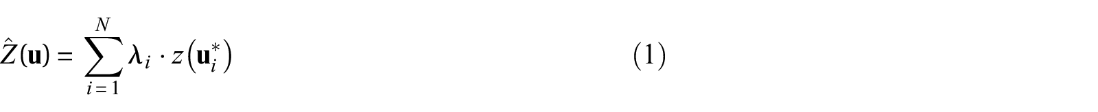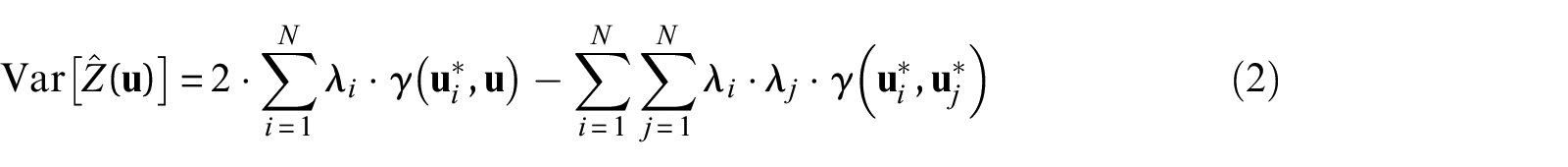The variance defined in Equation 2 is also known as kriging variance, and it is equal to zero at the observation points and takes positive values elsewhere. The variance, being a function of $\gamma$ , is also a function of the lag distance (h) between two points; the functional form between the variance and h is known as a variogram. Such a function allows for consideration of the spatial correlation, that takes into account the way a specific random variable varies in space.

The variogram can be bounded or unbounded and can take different analytical forms (Chilès and Delfiner, 2012; Webster and Oliver, 2007). The main parameters of the variogram are the nugget, the range, and the sill. The nugget is the value of the function for a lag distance equal to zero; the range is the lag distance for which the function becomes constant (i.e. the autocorrelation becomes zero); and the sill is the maximum value of the variogram and represents the maximum variance of the process. In this study, a spherical variogram function is adopted since it is among the most adopted for isotropic variables (Webster and Oliver, 2007):

$$\gamma (h)=\{\begin{array}{cc}c·[\frac{3}{2}·\frac{h}{a}-\frac{1}{2}·{\left(\frac{h}{a}\right)}^3]\hfill & \mathrm{for}h\le a\hfill \\ \multicolumn{1}{c}{c}& \mathrm{for}h>a\hfill \end{array}$$

(3)

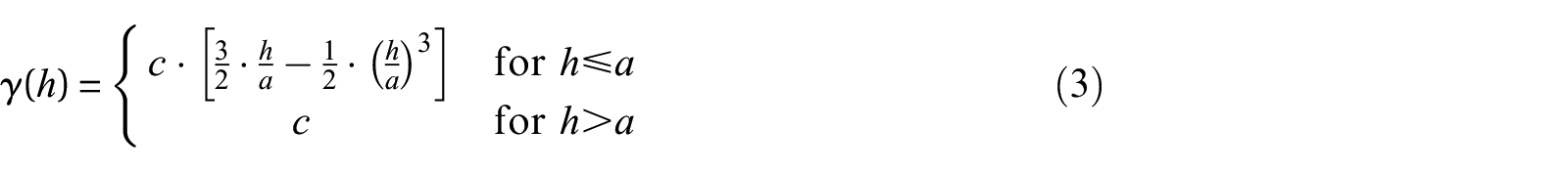
where a is the range, c is the sill, and the nugget is equal to zero.

Bayesian kriging

Figure 1 illustrates the main steps of the Bayesian kriging approach used in this article for a hypothetical problem domain. Let θ represent the parameters of the variogram (i.e. θ = {c,a}) that need to be estimated on the basis of newly available data D. θ may be considered as a set of random variables represented by (marginal/joint) probability distribution functions. According to the Bayesian paradigm, the distribution of θ can be updated with new observations (Box and Tiao, 1992):

$$f(\mathbf{\theta }|\mathbf{D})=C^{-1}·L(\mathbf{D}|\mathbf{\theta })·f(\mathbf{\theta })$$

(4)

where f(θ) is the prior distribution of the variogram parameters and identifies the available information on θ prior to the estimation and prior to the acquisition of more reliable data D (e.g. the V_S30 geophysical measurements), L(D|θ) is the likelihood function and characterizes the information from the newly available observations D, f(θ|D) is the posterior distribution describing the newly updated estimate of θ, and C is a normalization factor (De Risi et al., 2017). This approach allows the determination of the distributions of the parameters of the variogram. These distributions will facilitate the construction of a Bayesian predictor to be used in the kriging approach according to Equations 1 and 2.

Figure 1.

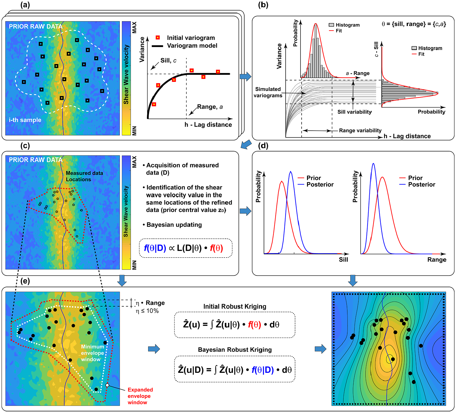
(a) Sampling of data and variogram fitting. (b) Definition of the prior distribution for sill and range. (c) Acquisition of more precise data and Bayesian updating setup. (d) Calculation of the posterior distribution of sill and range. (e) Initial and robust Bayesian kriging.

Informative priors f(θ) should be used in order to reflect the current state of knowledge about the parameters of interest (Pilz and Spöck, 2008). To elicit informative distributions, it is possible to use experience or prior data, that, in the early stages of the analysis, do not need to be highly informative. To obtain the prior distribution of the parameters of the variogram θ, a random sample of the prior data at random locations was performed; then, the natural logarithm of the samples is fitted with a variogram, and therefore the sill and range {c_i,ai_i} are obtained (Figure 1a). Repeating the sampling on the prior data many times allows a large number of variograms to be produced and hence a large number of potential values of sill and range. This sampling procedure is consistent with the so-called empirical Bayesian kriging (Krivoruchko and Gribov, 2014). The initial distributions of sill and range can be fitted with analytical distributions (Figure 1b) describing the prior knowledge of the parameters of the variogram f(θ).

If the generic random variable Z(u) is spatially distributed as a Gaussian random field, the likelihood function in Equation 4 is a multivariate normal with mean $({\mathit{z}}_D=\mathit{z}\left({\mathit{u}}_D^{*}\right))$ equal to the natural logarithm of the prior information at the locations $\left({\mathit{u}}_D^{*}\right)$ of the new N data D (Figure 1c), and the covariance matrix $\left({\mathbf{\Sigma }}_{\gamma }\left(\mathbf{\theta }\right)\right)$ is the one obtained using the variogram function that depends on θ. Therefore, the likelihood function can be written as:

$$L(\mathbf{D}|\mathbf{\theta })=(2\pi {)}^{-N/2}·{\left|{\mathbf{\Sigma }}_{\gamma }\right|}^{-1/2}·{\mathrm{e}}^{-\frac{1}{2}·{[\ln (\mathbf{D})-{\mathit{z}}_D]}^{\prime }·{\mathbf{\Sigma }}_{\gamma }^{-1}·[\ln (\mathbf{D})-{\mathit{z}}_D]}$$

(5)

where the dependency of ${\mathbf{\Sigma }}_{\gamma }$ on θ is omitted in the notation for simplicity. The covariance matrix is calculated for the natural logarithm of the random variable of interest.

From Equation 4, it is then possible to derive the posterior distribution of the variogram parameters f(θ|D) (Figure 1d). Either prior or posterior distribution of the variogram parameters can be used to propagate the uncertainties about θ in the final kriging estimation (Figure 1e). Depending on whether the prior or the posterior distribution of θ is used, the initial robust kriging (IRK) or the Bayesian robust kriging (BRK) is calculated by Equations 6 and 7, respectively:

$$\hat{Z}(\mathbf{u})=\int \hat{Z}(\mathbf{u}|\mathbf{\theta })·f(\mathbf{\theta })·d\mathbf{\theta }$$

(6)

$$\hat{Z}(\mathbf{u}|\mathbf{D})=\int \hat{Z}(\mathbf{u}|\mathbf{\theta })·f(\mathbf{\theta }|\mathbf{D})·d\mathbf{\theta }$$

(7)

where $\hat{Z}(\mathbf{u}|\mathbf{\theta })$ is calculated according to Equations 1 and 2 using as $z({\mathbf{u}}^{*})$ only the new data D (i.e. direct measurements). The robustness of the estimation is due to the fact that the uncertainties on the parameters of the variogram are propagated completely on the final estimation taking advantage of the total probability theorem (Jalayer et al., 2015); i.e. f(θ) and f(θ|D) represent the degree of confidence on θ (i.e. the weight of θ), and the integrals of Equations 6 and 7 are a weighted average of the kriging estimation based on the direct measurements D. In other words, the robust approach can be seen as a weighted average of kriging results where the weights are the probability density function (PDF) values of the parameters of the variogram.

Analogously to Equations 6 and 7, it is possible to compute maps of the robust kriging variance substituting $\hat{Z}(\mathbf{u}|\mathbf{\theta })$ with $\mathrm{Var}\left[\hat{Z}(\mathbf{u}|\mathbf{\theta })\right]$ evaluated according to Equation 2:

$$\mathrm{Var}[\hat{Z}(\mathbf{u})]=\int \mathrm{Var}\left[\hat{Z}(\mathbf{u}|\mathbf{\theta })\right]·f(\mathbf{\theta })·d\mathbf{\theta }$$

(8)

$$\mathrm{Var}\left[\hat{Z}(\mathbf{u}|\mathbf{D})\right]=\int \mathrm{Var}\left[\hat{Z}(\mathbf{u}|\mathbf{\theta })\right]·f(\mathbf{\theta }|\mathbf{D})·d\mathbf{\theta }$$

(9)

This variance quantifies, in a robust manner, the variability between the observations and the prediction. Furthermore, since the robust kriging is the expected value of $\hat{Z}$ for all the potential values of the model’s parameters, another estimation of the variance can be calculated as follows for the cases of IRK and BRK, respectively:

$${\sigma }_R^2[\hat{Z}(\mathbf{u})]=\int \hat{Z}{(\mathbf{u}|\mathbf{\theta })}^2·f(\mathbf{\theta })·d\mathbf{\theta }-{[\int \hat{Z}(\mathbf{u}|\mathbf{\theta })·f(\mathbf{\theta })·d\mathbf{\theta }]}^2$$

(10)

$${\sigma }_R^2\left[\hat{Z}(\mathbf{u}|\mathbf{D})\right]=\int \hat{Z}{(\mathbf{u}|\mathbf{\theta })}^2·f(\mathbf{\theta }|\mathbf{D})·d\mathbf{\theta }-{[\int \hat{Z}(\mathbf{u}|\mathbf{\theta })·f(\mathbf{\theta }|\mathbf{D})·d\mathbf{\theta }]}^2$$

(11)

This latter variance estimation provides the local variability associated with the robust assessment.

Conditioning the prior to measured data

The geographical coverage of the direct measurements D, in general, are not as extensive as for the less precise prior data. Therefore, the estimation of $\hat{Z}(\mathbf{u})$ by Equation 6 or 7 is limited to the geographical coverage of D (e.g. the minimum envelope represented in Figure 1e as dashed white line) in which only interpolation is performed, or to a slightly larger area (e.g. the expanded envelope window in Figure 1e represented in a dashed red line, obtained expanding the minimum envelope domain of a small percentage $\eta$ of the range, for example, $\eta$ ≤ 10%) for which both interpolation and extrapolation are needed. The limitation on the extrapolation area allows limiting the variability of the extrapolation. For example, to a value of $\eta$ equal to 10% corresponds a variance equal to the 15% of the sill (Equation 3), allowing the control of this parameter in the extrapolation area by the user. However, the domain can be limited using any other physically informed rationale; for example, the extrapolation could be contained only within a specific geological feature (e.g. a basin within a mountain range with significantly different geological features).

Several approaches exist in the literature to anchor regional data to local observations (Miano et al., 2016; Worden et al., 2010). Building upon these methods, to extend the estimation to a larger geographical area, for example, the one covered by the prior data, it is possible to condition the prior data to the more precise new data D according to the following expression (Eaton, 1983):

$$z(\mathbf{u}|\mathbf{\theta })=z(\mathbf{u})+{\mathbf{\Sigma }}_{\gamma ,{\mathit{z}}_D\ln (\mathbf{D})}·{\mathbf{\Sigma }}_{\gamma ,\ln (\mathbf{D})\ln (\mathbf{D})}^{-1}·[\ln (\mathbf{D})-{\mathit{z}}_D]$$

(12)

where $z(\mathbf{u})$ represents the logarithm of the prior data, ${\mathbf{\Sigma }}_{\gamma ,z_D\ln (\mathbf{D})}$ is the cross-covariance matrix for the logarithm of the prior values in correspondence of the new data $(z_D)$ and the logarithm of the new data (ln(D)), and ${\mathbf{\Sigma }}_{\gamma ,\ln (\mathbf{D})\ln (\mathbf{D})}$ is the covariance of the logarithm of the new data. Both covariance matrices can be obtained using the variogram function for which the prior or posterior distributions of the parameters are employed.

This well-consolidated conditioning can be integrated and improved using the robust approach discussed previously. The estimates z(u|θ) obtained from Equation 12 can be used in Equation 6 or 7 (using either prior or posterior distribution) to obtain robust conditioning of the initial estimates on the new measurements allowing to propagate the uncertainties of the variogram parameters into the conditioned map. Therefore, it is possible to obtain updated robust maps with a geographical extent identical to the prior data.

The Kathmandu valley case

In this study the shear wave velocities provided by the USGS V_S30 model (Allen and Wald, 2009) were used as prior data. The V_S30 map is shown in Figure 2a. The map describes well the general distribution of the metamorphic bedrock surrounding the valley and characterizes the inner distribution of valley sediments of lacustrine and fluvio-deltaic origins (Shrestha et al., 1998). Further information on the geotechnical parameters associated with these soils are provided in Gilder et al. (2020). On the same plot, the area of the valley sediments identified from the geological map is enclosed within the blue line, and an example of random sampling across the greater area is also shown. For this specific study, it was observed that 30 samplings are the minimum number to fit a variogram in a stable manner. Repeating the sampling 1000 times, 1000 variogram functions are generated (gray lines in Figure 2b) from which it has been possible to obtain empirical distributions of range and sill values.

Figure 2.

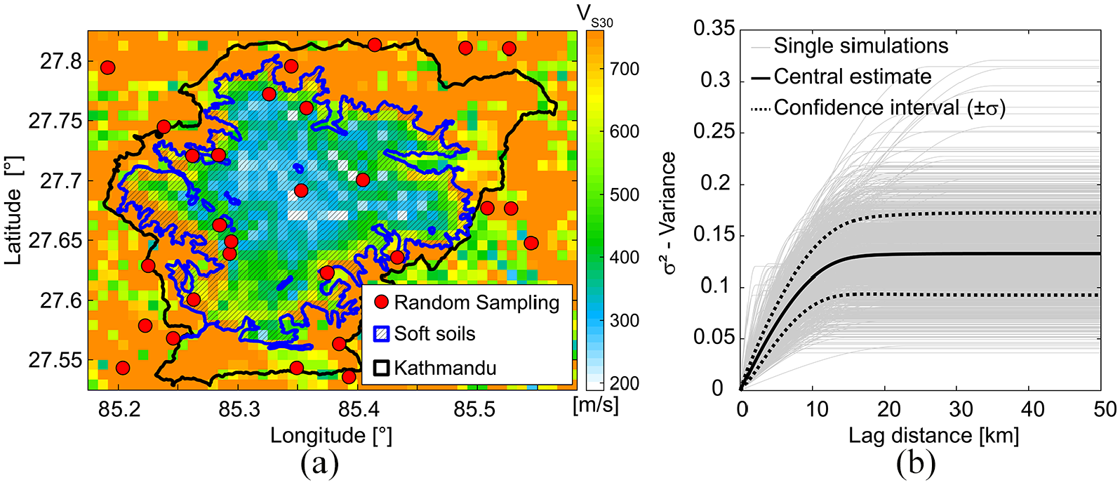
(a) USGS V_S30 database for Kathmandu and example of random sampling. (b) Initial variogram functions; (0.05°≈ 5.6 km).

To investigate the sensitivity of the sampling to the dimension of the sampling domain, two different areas were investigated: (a) the larger area corresponding to the geographical extent in Figure 2a, and (b) a smaller area corresponding to the area of sediments, enclosed in the blue domain in Figure 2a. Figure 3 shows the distributions of sill and range for both the larger area (Figure 3a and b) and the soft soil area (Figure 3c and d). For both the c and a parameters of the variograms, a generalized extreme value (GEV) distribution (Kotz and Nadarajah, 2000) was found to be the model that best fit the data compared to other simple models (e.g. Log-Normal, Normal, Weibull). In this work, sill and range are assumed to be uncorrelated. Only a small reduction in the central value of the range and the dispersion can be observed between the distributions obtained for the two sampling domains. The fitted distributions can be used as informative priors in Equation 4. Figure 3a and c, as well as Figure 3b and d, shows very similar results. Although very similar, these two priors are used here to check whether the posterior is sensitive to the extent of the sampling domain. The triplets of parameters presented in parenthesis in Figure 3 are the parameters of the GEV, that is, the shape factor p₁, the scale factor p₂, and the location parameter p₃, respectively. Equation 13 shows the analytical expression of the GEV PDF for a generic variable x:

$$f(x)=\left(\frac{1}{p_2}\right)\exp [-{(1+p_1\frac{x-p_3}{p_2})}^{-\frac{1}{p_1}}]{(1+p_1\frac{x-p_3}{p_2})}^{-1-\frac{1}{p_1}}$$

(13)

Figure 3.

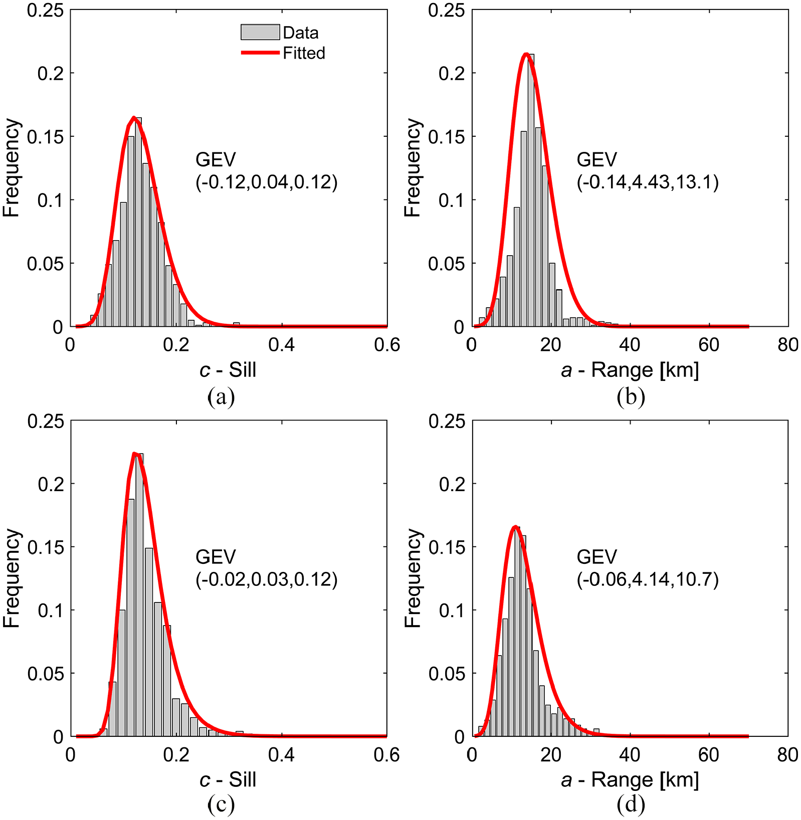
(a, c) Distributions of the sill. (b, d) Distributions of the range. Results for the (a, b) greater area and (c, d) sediment area.

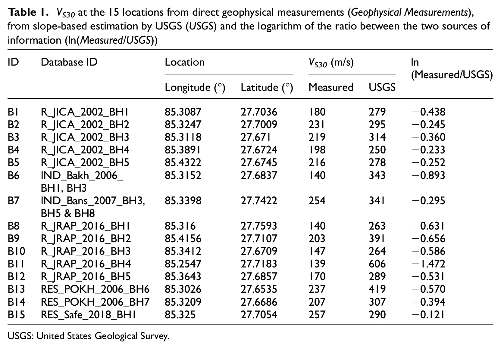
As presented in Gilder et al. (2020), 18 direct geophysical measurements of V_S30 are available in the Kathmandu valley (Figure 4a), also see Gilder et al. (2019) for the database SAFER/GEO-591. Since some measurements are in the same location, they are averaged and considered only once. Therefore, 15 measured V_S30 were available for the analysis presented in this article. Table 1 lists the V_S30 values obtained from both the downhole seismic tests and the USGS model. The USGS values tend to systematically overestimate the available borehole data for the Kathmandu valley, especially for the boreholes close to steep locations (e.g. B11), as also observed in Stewart et al. (2014). Moreover, as observed by Allen and Wald (2009), the lower elevations provided the worst estimates. Some measured V_S30 values are particularly low with respect to the USGS estimations (e.g. B6, B8, B10, B11, B12); these sites correspond to locations that are underlain by Quaternary (i.e. recent deposits or Talus Cone deposits), as well as the Plio-Pleistocene sediments.

Figure 4.

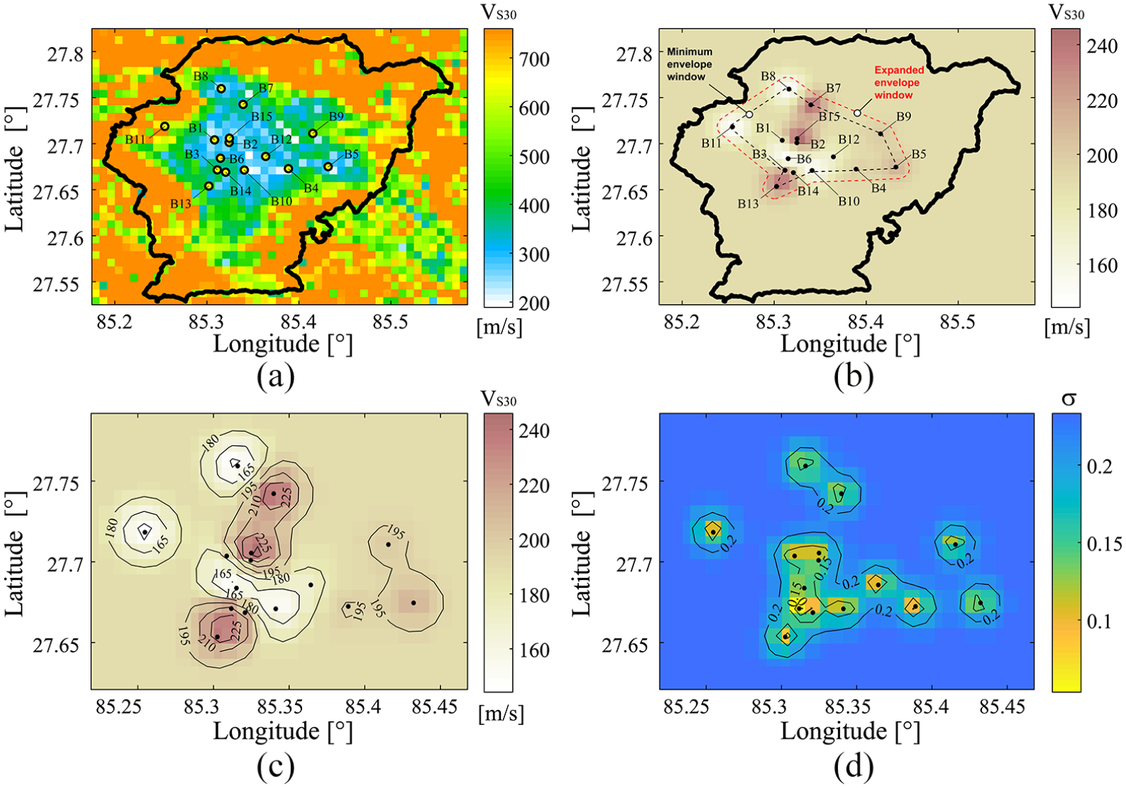
(a) Location of the measurements. (b) Ordinary kriging based on the measurements and variogram. (c) Ordinary kriging for the small window. (d) Kriging standard deviation; (0.05°≈ 5.6 km).

Table 1.

V_S30 at the 15 locations from direct geophysical measurements (Geophysical Measurements), from slope-based estimation by USGS (USGS) and the logarithm of the ratio between the two sources of information (ln(Measured/USGS))

ID	Database ID	Location		VS30 (m/s)		ln (Measured/USGS)
		Longitude (°)	Latitude (°)	Measured	USGS
B1	R_JICA_2002_BH1	85.3087	27.7036	180	279	−0.438
B2	R_JICA_2002_BH2	85.3247	27.7009	231	295	−0.245
B3	R_JICA_2002_BH3	85.3118	27.671	219	314	−0.360
B4	R_JICA_2002_BH4	85.3891	27.6724	198	250	−0.233
B5	R_JICA_2002_BH5	85.4322	27.6745	216	278	−0.252
B6	IND_Bakh_2006_BH1, BH3	85.3152	27.6837	140	343	−0.893
B7	IND_Bans_2007_BH3, BH5 & BH8	85.3398	27.7422	254	341	−0.295
B8	R_JRAP_2016_BH1	85.316	27.7593	140	263	−0.631
B9	R_JRAP_2016_BH2	85.4156	27.7107	203	391	−0.656
B10	R_JRAP_2016_BH3	85.3412	27.6709	147	264	−0.586
B11	R_JRAP_2016_BH4	85.2547	27.7183	139	606	−1.472
B12	R_JRAP_2016_BH5	85.3643	27.6857	170	289	−0.531
B13	RES_POKH_2006_BH6	85.3026	27.6535	237	419	−0.570
B14	RES_POKH_2006_BH7	85.3209	27.6686	207	307	−0.394
B15	RES_Safe_2018_BH1	85.325	27.7054	257	290	−0.121

USGS: United States Geological Survey.

Initially, the measured V_S30 values are used in the ordinary kriging (Figure 4b and c) and to compute the standard error $(\sigma =\sqrt{\mathrm{Var}[\hat{Z}(\mathbf{u})]})$ associated with the geostatistical analysis (Figure 4d). These results are presented here for comparison with the results presented later in the article. As discussed earlier, the error is minimum in correspondence of the measurement location and increases moving away from these measurements. The error map allows the identification of sites for future field investigations (e.g. the blue area in Figure 4d). However, it is not possible to account only for the reduction in the prediction error; a risk-based approach should be used. Further constraints must be considered (e.g. the exposure, the seismic vulnerability of the assets at stake). Hence, identifying locations for future geotechnical field investigations should be done to optimize the inevitable compromise between the error reduction (in a geostatistical sense) and the need of precise geotechnical data in areas where the risk may be highest (e.g. Gilder et al., 2018).

Figure 5 shows the difference between the variograms obtained using both the measured data (i.e. black cross markers and black lines) and the two generic random samplings from the USGS maps (i.e. the square markers and dashed lines in Figure 5a and 5b). As shown in Figure 2b, the two simulations in Figure 5a and b are selected to show the large variability that can be obtained in terms of initial variograms and its fit. The plots emphasize the significant difference that exists between a variogram generated according to the proposed sampling procedure (i.e. dashed curves in Figure 5a and b, respectively) and the one obtained according to a straightforward ordinary procedure (i.e. the black solid curve in Figure 5).

Figure 5.

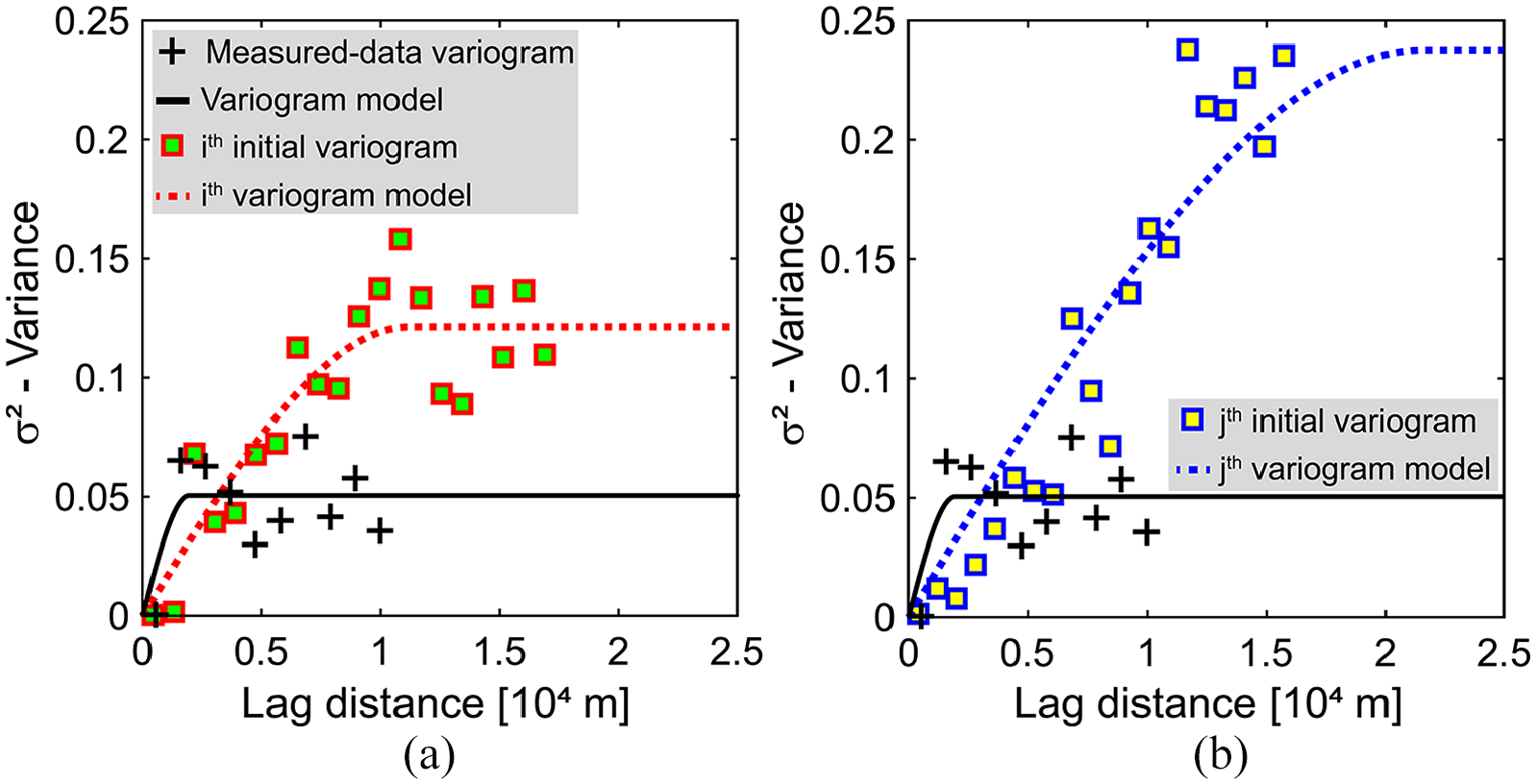
Comparison of the variograms calculated using the measured data and two random samplings from the USGS map.

The direct geophysical measurements can be used in the likelihood function defined by Equation 5. Integrating Equation 5 and the prior distributions of the parameters of the variogram, it is possible to obtain the posterior distributions of the parameters of the variogram (Figure 6).

Figure 6.

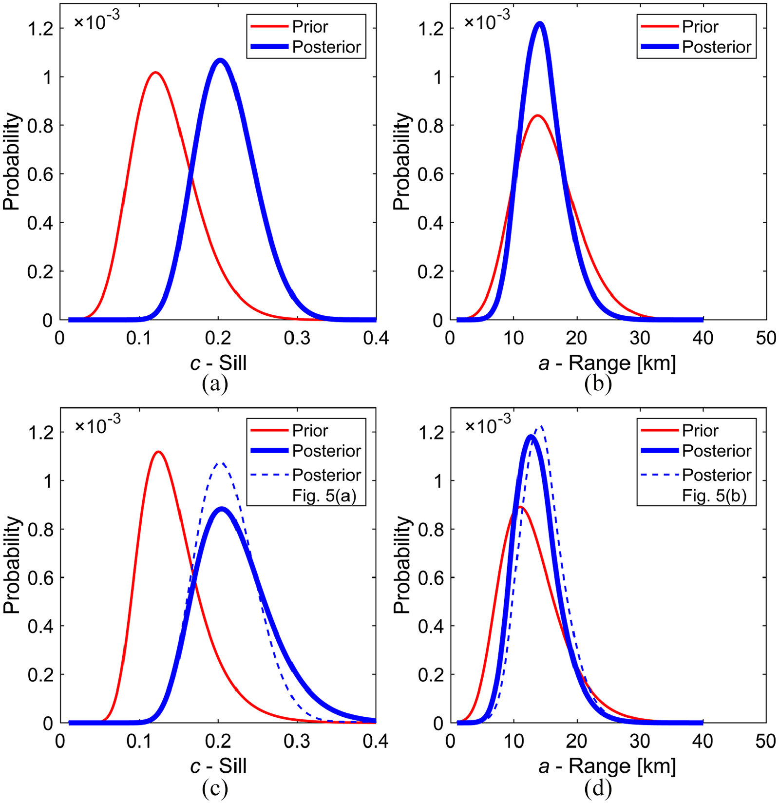
(a, c) Prior and posterior distributions of the sill. (b, d) Prior and posterior distributions of the range. Results for the (a, b) larger area (entire Kathmandu Valley) and (c, d) sediment area (soft soil area) as per Figure 2a.

To demonstrate the influence of the prior distribution, results are shown for both the larger geographical (Figure 6a and b) and the sediment (Figure 6c and d) sampling domains. Figure 6a and c shows that the distribution of the sill shifts toward higher values, its variability remains constant, and the shape of the function tends to lose the positive skewness becoming more symmetric for the larger geographical domain meanwhile retaining the right skewness for the sediment area sampling domain. Figure 6b and d shows that the distribution of the range shifts to higher values for the domain containing sediments only. Nevertheless, for both sampling domains, variability is lower, and skewness is toward higher values of the range. The results presented in Figure 6 demonstrate that the maps obtained using the posterior parameters will have a larger variability for the same amount of lag distance. Therefore, posterior maps will present a more gradual variation of estimates and will reflect the fact that the V_S30 is not purely distributed according to the topographical features. Moreover, it can be observed that the posteriors obtained using the two sampling domains are similar (continuous and dashed blue lines in Figure 6c and d). Both the prior and the posterior distributions of the parameters of the variogram can be used in Equations 6 and 7 to obtain robust kriging estimations. Figure 7a and c shows the IRK, and Figure 7b and d shows the BRK. In addition, minimum and expanded envelope domains are shown in gray and red dashed lines. Regarding the comparison of IRK and BRK, the results are very similar. However, for both IRK and BRK cases, the results are dissimilar from the results of the ordinary kriging presented in Figure 4c, especially with respect to the contour levels of V_S30.

Figure 7.

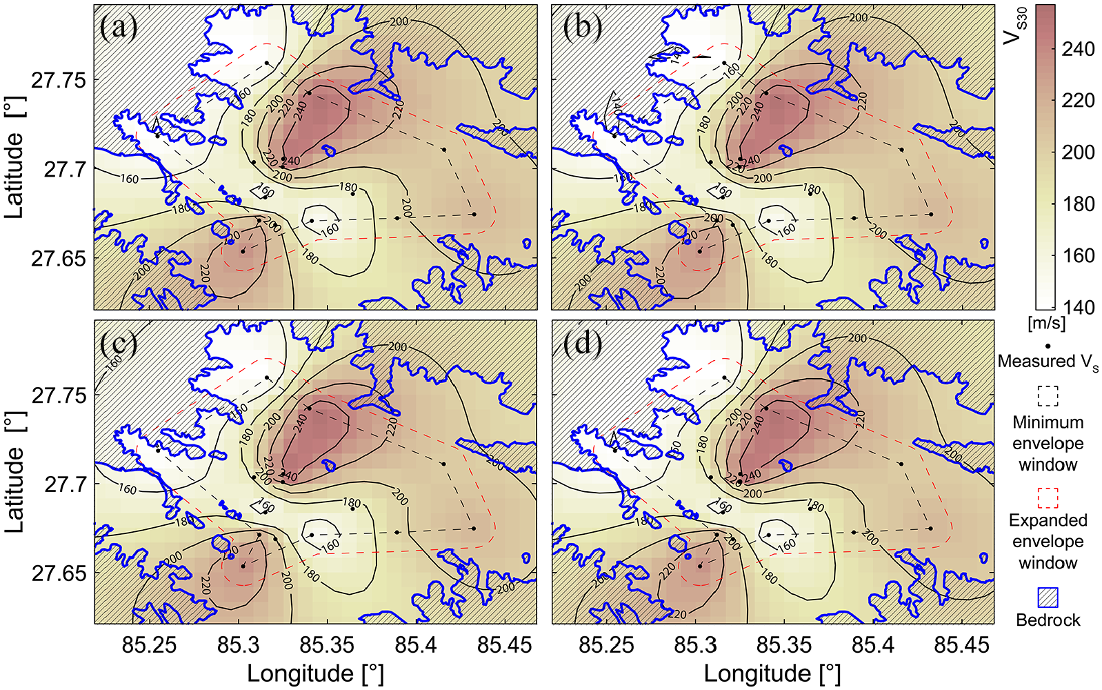
(a, c) Initial robust kriging (IRK) and (b, d) Bayesian robust kriging (BRK). Results for the (a, b) larger area and (c, d) soft soil area; (0.05°≈ 5.6 km).

Figure 7a and c, as well as Figure 7b and d, shows almost identical results. It is possible to conclude that the robust kriging, for the considered case study, is not sensitive to the shape of the priors of the variogram parameters. Therefore, in the following discussion, only the results obtained considering the larger sampling domain are presented. The larger sampling domain is preferred as it will allow a broader use for future updates of results from additional investigations done in the valley.

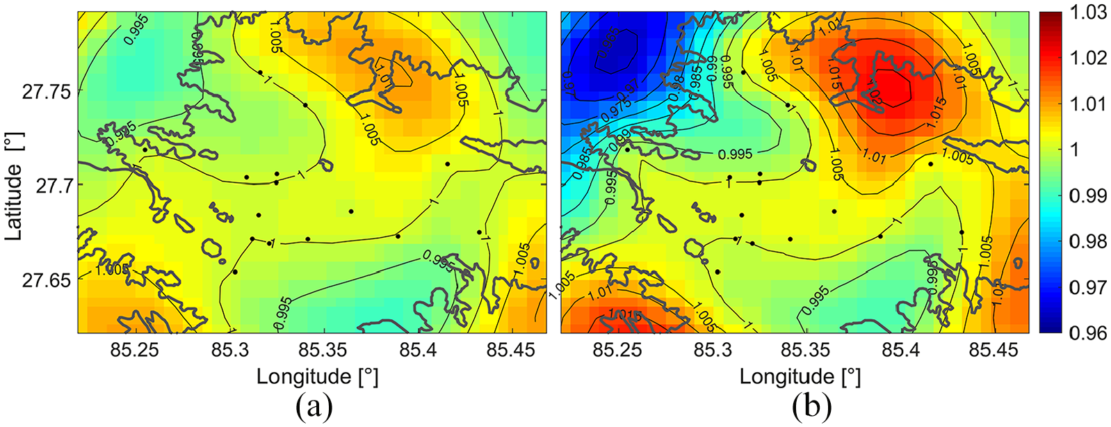
As expected, also high similarities between the results obtained with the posterior and the prior distributions of the parameters of the variograms can be observed. Figure 8 shows the ratio between the V_S30 estimation obtained with the different hypotheses. It is possible to conclude that maximum variation of it is in the range of ±3% for this case study; therefore, the number of measured data is still too small to obtain significant variation with the Bayesian approach.

Figure 8.

Ratio between BRK and IRK for the larger area and the soft soil area: (a) the results presented in Figure 7b and a. (b) the results presented in Figure 7d and c.

In addition to previous results, considering only the larger sampling domain, the maps of the standard deviation for the kriging estimation are also presented for both IRK and BRK. Specifically, Figure 9a and b shows the kriging variance obtained from Equations 8 and 9, respectively. Figure 9c and d shows the variance obtained from Equations 10 and 11, respectively. From Figure 9a and b, it is possible to conclude that the kriging variability for the BRK is slightly larger than the IRK one; therefore, although the estimation presented in Figure 7a and b is similar, the variability for the BRK is slightly larger, as expected looking at the posteriors of the sill. However, results presented in Figure 9c and d show that the weighted averaging estimation performed for the BRK leads to a lower local variability.

Figure 9.

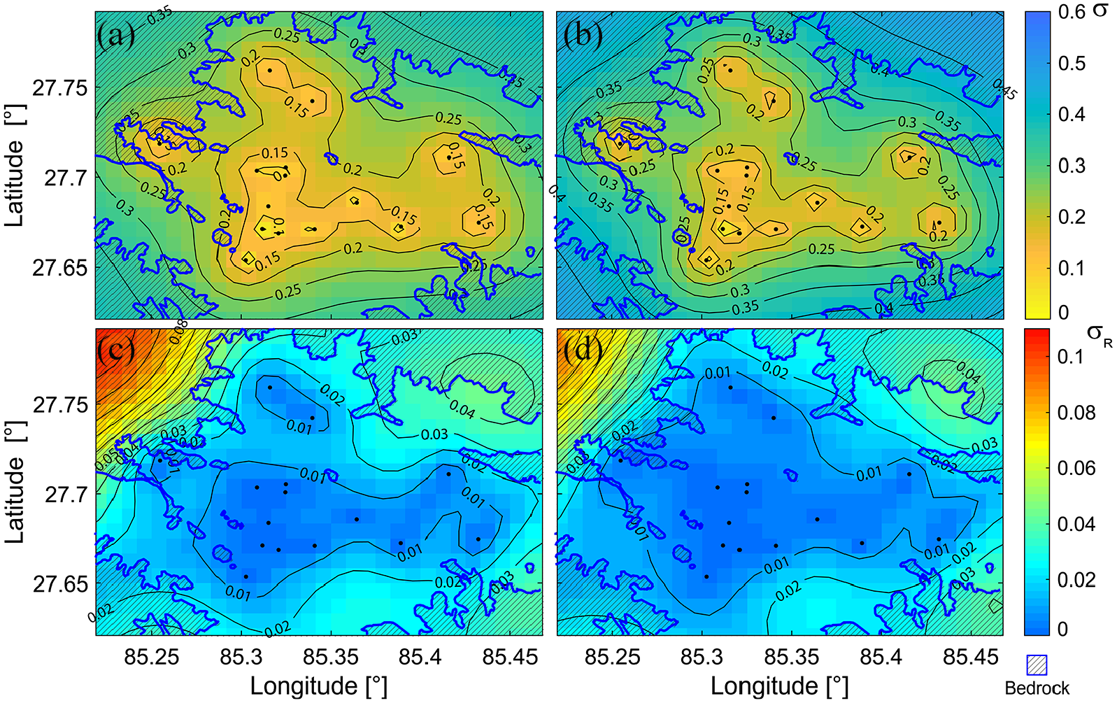
Kriging standard deviation for (a) initial robust kriging (IRK) as per Equation 8 and (b) Bayesian robust kriging (BRK) as per Equation 9. Local standard deviation for (c) IRK as per Equation 10 and (d) BRK as per Equation 11; (0.05°≈ 5.6 km).

Conditional V_S30 map

The 15 geophysical measurements can be used to condition prior data according to Equation 12. Figure 10a and b show the initial USGS V_S30 map and the same map with conditioned V_S30 values.

Figure 10.

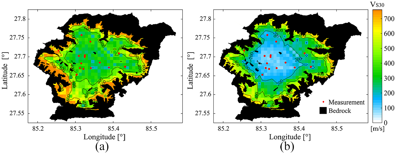
Shear wave velocity maps: (a) USGS estimates. (b) USGS estimates conditioned on the measurements; (0.05°≈ 5.6 km).

For the robust application, only the posterior distribution of the parameters of the variograms is used (i.e. the parameters distributed according to the blue curves in Figure 6a and b). The initial values are reduced by the measured values, and the distribution of the V_S30 values in the central part of the valley is smoothed. The main effect on the result can be observed where there is a higher concentration of measurements. No significant variation of the V_S30 values can be observed far from the locations of the measurements. In this case, the geologic bedrock is overlaid on the map (black area in Figure 10).

Comparisons

For comparison purposes, in Figure 11, the two contour maps of shear wave velocity obtained through BRK (Figure 7b) and USGS estimates conditioned to the measurements (Figure 10b) are compared with the geology maps given in the companion paper Gilder et al. (2020). The first map, originally developed by Yoshida and Igarashi (1984), provides information on the geology inferred from geomorphology (Figure 11a and b). The second map, developed by Shrestha et al. (1998), provides geological information as a result of engineering soil classification (Figure 11c and d).

Figure 11.

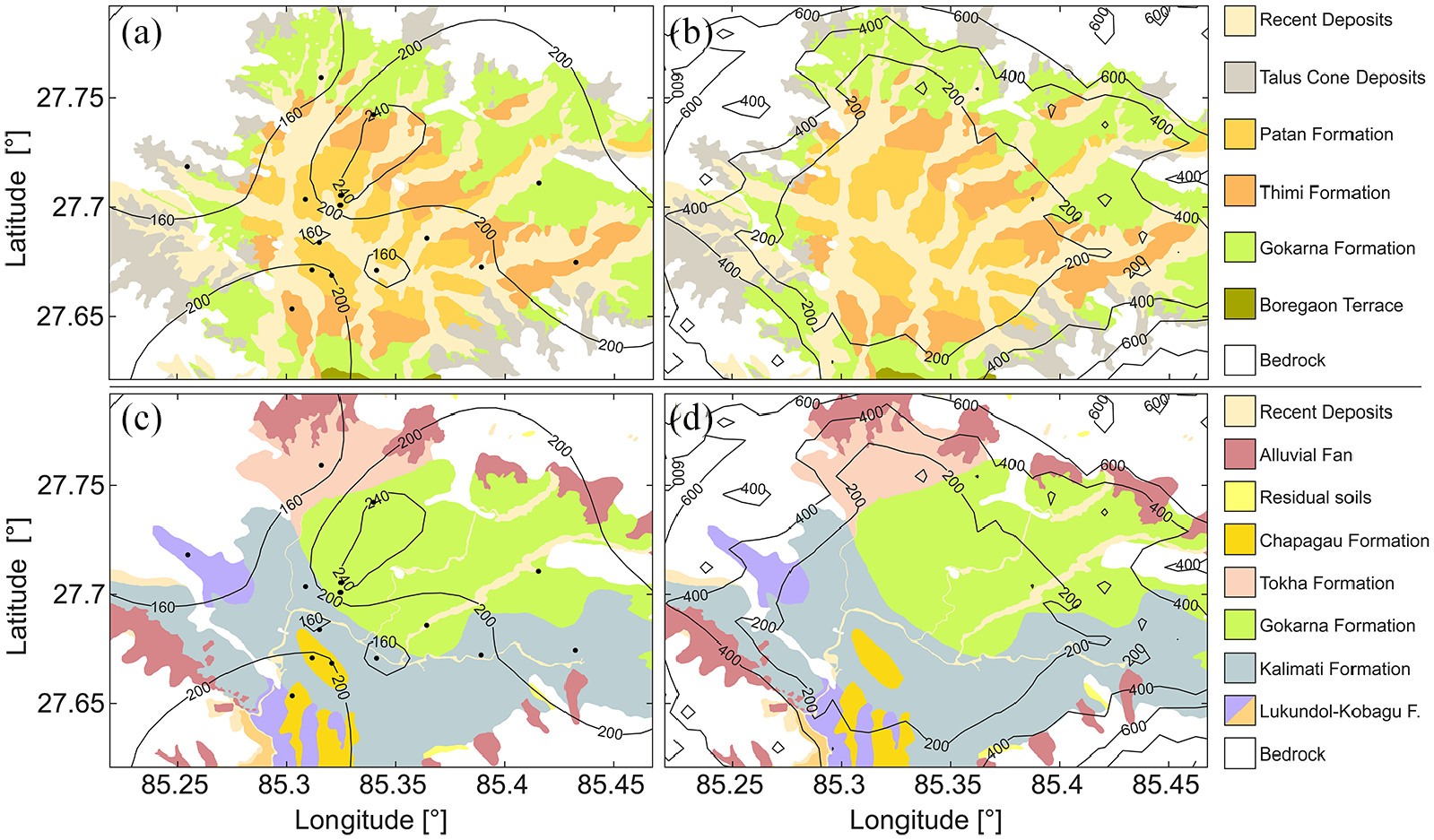
Overlay of the geology maps with the contours of the of V_S30 obtained considering (a, c) only the geophysical measurements and (b, d) the USGS estimates conditioned to the geophysical measurements. (a, b) Geology maps shown in Gilder et al. (2020) based on Yoshida and Igarashi (1984). (c, d) Geology maps shown in Gilder et al. (2020) based on Shrestha et al. (1998); (0.05°≈ 5.6 km).

Figure 11a shows how the interpolated results (i.e. in the minimum envelope domain) describe the variability of the shear wave velocities in the central part of the valley where the sediments are present very well. Figure 11b provides an update to the prior assumptions made in the USGS topographical model, and the geophysical data indicating the inner portion of the valley has even lower values than the global model, due to the specific deposits present in this area (both recent river deposits and tidal flat, coupled with an underlying silt lake deposit—Kalimati Formation). A critical aspect is realized when the engineering geological map is compared to the results, that is, sediment distributions based on origin and grain size. The overlay in Figure 11c shows that the kriging provides a distinction between the two main engineering soils present in the valley (Gokarna and Kalimati Formations). It may be expected that the Gokarna Formation will have higher values of V_S30, as it contains sand/gravel layers, interlayered within silt and clay. Alternatively, the Kalimati Formation (in the southern central valley) is a more homogeneous engineering material comprising a clay/silt which is expected to exhibit lower values of V_S30.

It is acknowledged that there remains a need for improvement of some aspects of the kriged distribution, as seen by the two boreholes in the upper-left part of Figure 11c; they are located in particularly soft/loose recent deposits, which is producing an imprecise estimation toward the bedrock, and potentially uninformative distribution across the remaining sediments in that portion of the valley. Where the bedrock might be expected to be reasonably shallow in these upper topographies, the V_S30 data are not available. To summarize, Figure 11b and d showing the USGS values conditioned on the geophysical measurements can aid in providing lower values for a model spanning the entire valley. Alternatively, Figure 11a and c reflects the engineering soil classification, with local greater resolution information, very well.

Conclusions

This article details a new approach to extract controlled-confidence estimations from available geotechnical data in data-scarce regions. Ordinary kriging was used to draw maps representing the geographical variability of V_S30, which can aid decision in locating new geotechnical investigations. A Bayesian kriging approach has been proposed to combine several layers of data. Specifically, the slope-based V_S30 estimates provided by the USGS have been used as prior, and direct geophysical measurements are used to inform the likelihood model. The posterior distributions obtained by means of the Bayesian approach can be used to obtain a robust kriging interpolation/extrapolation. Finally, using the posterior variograms, a procedure for conditioning the prior data to the geophysical measurements has been proposed, allowing extension of the estimations to a geographical coverage larger than that of the (more precise) direct estimations.

The procedures have been applied to the case study of the Kathmandu valley, Nepal, and the results have been compared with the geological information for the valley. Both ordinary and Bayesian kriging perform best in the central part of the valley, where the density of observations is larger; moreover, the proposed methodology provides more gradual change of the geotechnical property with respect to the ordinary kriging that instead works efficiently mainly around measurements and changes in a more abrupt manner. From the conditioned prior data, it has emerged that there is a substantial reduction in the initial values, and the distribution tends to change mainly where the concentration of observation is high providing suitable results for extrapolations. The progression of the increasing value of shear wave velocity from the center toward the mountains remains evident.

In the case study, the number of observations available does remain insufficient (i.e. 15 measurements) for such a large area to produce significantly different results between IRK and BRK. However, the novel approach proposed allows for full control of the confidence of the interpolation, and the robust approach allows for a characterization of the variance at the local level.

Several potential improvements should be explored in future work; for example, including the heterogeneity of the variables that were not discussed in this study. The sampling scheme adopted to create the priors can be modified considering a different technique. Moreover, variogram parameters could be considered jointly. Finally, advanced simulation routines may be used to solve the Bayesian problem.

Supplemental Material

sj-zip-1-eqs-10.1177_8755293020970977 – Supplemental material for The SAFER geodatabase for the Kathmandu valley: Bayesian kriging for data-scarce regions

Supplemental material, sj-zip-1-eqs-10.1177_8755293020970977 for The SAFER geodatabase for the Kathmandu valley: Bayesian kriging for data-scarce regions by Raffaele De Risi, Flavia De Luca, Charlotte EL Gilder, Rama Mohan Pokhrel and Paul J Vardanega in Earthquake Spectra