Fast Evaluation of Deep Neural Network (DNN) for Past Dataset in Incremental Learning

Abstract

During the operation of a system including a deep neural network (DNN), new input values not included in the training dataset are given to the DNN. In such a case, the DNN may be incrementally trained with the new input values; however, additional training may reduce the accuracy of the DNN in regard to the dataset that was previously obtained and used for the past training. The effect of the additional training on the accuracy for the past dataset needs to be evaluated, but evaluation by testing all the input values included in the past dataset takes time. Therefore, we propose a new method to evaluate the effect on the accuracy for the past dataset, in which the gradient of the parameter values (such as weight and bias) for the past dataset is extracted by running the DNN before the training. After the training, the effect on the accuracy with respect to the past dataset can be calculated fast from the gradient and update differences of the parameter values. To show the usefulness of the proposed method, we present experimental results with several datasets. The results show that the proposed method can estimate the accuracy change by additional training in a short constant time.

1. Introduction

The introduction of machine-learning technologies in various industrial fields has been advancing. Among those technologies, deep neural networks (DNNs) are being widely applied. In addition to replacing human labor, in a number of fields, DNNs are outperforming people. DNNs are trained with a dataset composed of pairs of input values and their corresponding expected output values. A part of the dataset is used for training DNNs, and the rest is used to evaluate the trained DNNs. In the training, when input values are included in the training dataset, values of parameters such as weights and bias are adjusted so that the expected output values are more likely to be obtained. After the training is completed, the test dataset is used to measure the probability of obtaining the expected output value as expected. This probability—called accuracy—indicates the validity of the developed DNNs. However, the accuracy measured during development is only that with respect to the existing dataset retained at that time. When input values that are not included in the existing dataset are input to a DNN, the output values are not exclusively those expected; consequently, the DNN is less accurate during operation than during its development.

When the accuracy of DNNs decreases during operation, it is useful to apply incremental learning (Crankshaw et al., 2014; Leo & Kalita, 2024; Luo et al., 2020; Wang et al., 2024b; Xiao et al., 2014; Zhou et al., 2023), in which a DNN is trained by using a dataset newly acquired during operation. In incremental learning, parameter values of the DNN are adjusted to improve the accuracy of the newly acquired dataset. However, the result of the adjustment also affects the accuracy of the dataset used in the previous trainings. When the accuracy for the past dataset decreases, the updated DNN is not easily adopted. If a system operator finds that a concept drift of input values happens, the decrease in accuracy for the past dataset can be ignored because the past dataset and its similar data are not input thereafter. However, since the operator is not always able to detect changes in the distribution of input values, they can rarely be confident that the decrease in the accuracy for the past dataset can be ignored. Even if the distribution changes due to concept drift, a part of the input values before the change may still be included after the change. In such cases, it should maintain a certain level of accuracy for the past dataset. From the above considerations, the decision to use the updated DNN is based on the accuracy for the past dataset and the results of the concept drift evaluation. In addition, in a number of systems, the decision to adopt or discard the updated DNN should be made as soon as possible to prevent losing business opportunities. To grasp the effect of additionally conducted training on the accuracy of the past dataset, it is sufficient to run the updated DNN with all the input values included in the past dataset and acquire its accuracy again. However, when the past dataset is huge, the test takes a long time to execute. In other words, the accuracy of the DNN cannot be evaluated quickly by testing.

Therefore, we propose a fast evaluation method for the effect of additional training on the accuracy for the past dataset (Sato et al., 2018). In the proposed method, the gradient of the parameter values is extracted by executing the DNN with the input values in the past dataset before the DNN update. After the additional training, the effect on the accuracy of the past dataset is evaluated on the basis of the gradient and the update differences of parameter values of the DNN. We also leverage a linear regression analysis to estimate the increase/decrease in accuracy. The calculation to be conducted after additional training does not depend on the number of input values in the past dataset. Therefore, even if the past dataset is huge, applying the proposed method enables the effect of additional training to be evaluated fast. To demonstrate the usefulness of the proposed method, we show the experimental results using the MNIST, Fashion MNIST, and the German Traffic Sign Recognition Benchmark (GTSRB) datasets.

The rest of this paper is organized as follows. In Section 2, the structure of DNNs and a flow of incremental learning are defined. The problem that we focus on in incremental learning is also described. In Section 3, the proposed method is presented on the basis of several calculation formulas. In Section 4, the results of experiments applying the proposed method to three datasets are shown. In Section 5, the usefulness of the proposed method is evaluated and discussed on the basis of the experimental results. In Section 6, related work is described, and in Section 7, the conclusions drawn from this study are presented.

2. Preliminaries

2.1. Deep Neural Networks (DNNs)

For an arbitrary DNN, denoted as $N$ , handling a classification problem of class $c(c>1)$ , $I$ is taken as the number of neurons making up $N$ , and each neuron (in any layer) is denoted as $n_i(1\le i\le I)$ . Also, $J_i$ is taken as the number of parameters used to calculate the value of $n_i$ , and the parameter itself is denoted as $[w_{i,1},\dots ,w_{i,j},\dots ,w_{i,J_i}]$ . Note that if $n_{i_1}$ and $n_{i_2}$ are included in different layers, $J_{i_1}$ and $J_{i_2}$ can be different. A vector obtained by combining the parameters of all neurons is defined as $\mathbf{W}=[w_{1,1},\dots ,w_{1,J_1},w_{2,1},\dots ,w_{2,J_2},\dots ,w_{I,1},\dots ,w_{I,J_I}]$ . For a multilayer perceptron (MLP), for example, these parameters correspond to weights and biases. The formula for calculating the value of each neuron by using these parameters is not described in this paper.

For an arbitrary input value $x^m$ , the corresponding expected output value is expressed as $t(x^m)$ , which represents the identifier of the classification class to which $x^m$ belongs. When $x^m$ is input to $N$ , the output value returned by $N$ is expressed as $\mathbf{y}(x^m)$ , which corresponds to the c-dimensional vector $\mathbf{\text{y}}(x^m)=[y_1^m,\dots ,y_k^m,\dots ,y_c^m]$ . The $y_k^m$ value for each dimension represents the probability that the input value $x^m$ belongs to class $k$ . If $y_k^m$ has the largest value in $[y_1^m,\dots ,y_k^m,\dots ,y_c^m]$ , class $k$ is denoted as $fst(\mathbf{y}(x^m))$ . That is, $\mathrm{\forall }{y}_k^m\cdot y_k^m\le y_{fst(\mathbf{y}(x^m))}^m$ holds. When $fst(\mathbf{y}(x^m))=t(x^m)$ holds, it is said that $N$ can correctly classify $x^m$ . Likewise, if $y_k^m$ has the second largest value, class $k$ is denoted as $snd(\mathbf{y}(x^m))$ . Specifically, $\mathrm{\forall }{y}_k^m\cdot y_k^m\ne y_{fst(\mathbf{y}(x^m))}^m\Rightarrow y_k^m\le y_{snd(\mathbf{y}(x^m))}^m$ holds.

Since the number of layers, neurons, and parameters are generalized in the definition of DNNs, and types of activation functions are not specified, the proposed method can be applied to any neural network in which the gradient of parameters is computable.

2.2. Incremental Learning

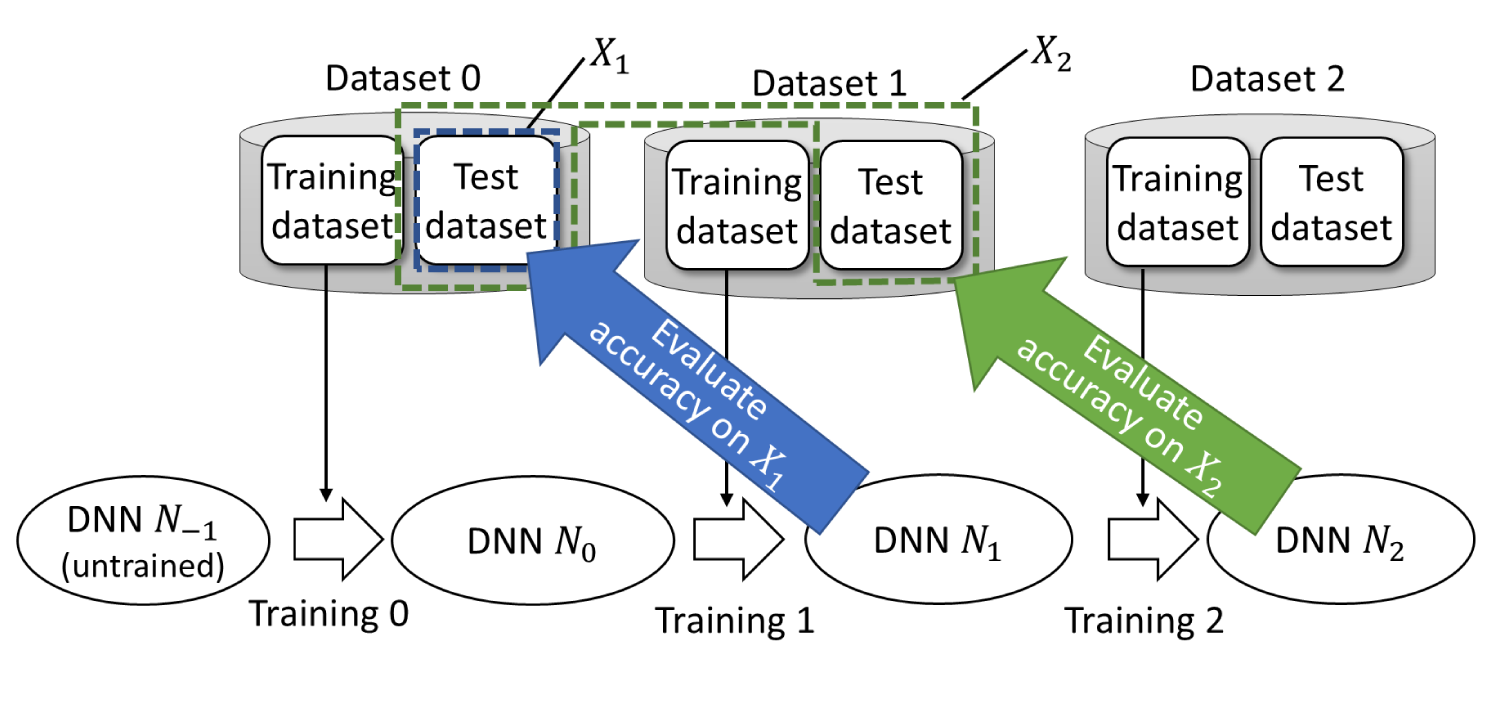
The flow of incremental learning is shown in Figure 1. An untrained DNN $N_{-1}$ is trained first by using the training dataset of Dataset 0. The trained DNN $N_0$ is evaluated by using the test dataset of Dataset 0. After testing, $N_0$ starts to be used. During its use, Dataset 1 is newly acquired. At that time, $N_0$ is trained again using the training dataset of Dataset 1, and the updated DNN $N_1$ is evaluated in the same way using the corresponding test dataset. However, $N_1$ does not always maintain sufficient accuracy for Dataset 0. Accordingly, the effect of training 1 on the accuracy for Dataset 0 needs to be evaluated. That necessity holds for the following incremental learning.

Figure 1.

Flow of incremental learning. An untrained deep neural network (DNN) $N_{-1}$ is trained by the training dataset of Dataset 0. The trained DNN $N_0$ is evaluated by using the test dataset of Dataset 0. After that, $N_0$ is trained again and updated to $N_1$ using the training dataset of Dataset 1 that is newly obtained. The updated DNN $N_1$ is evaluated by using the test dataset of Dataset 1. At that time, $N_1$ should also be evaluated for the test dataset of Dataset 0, which is denoted as $X_1$ . Similarly, DNN $N_2$ should be evaluated not only for the test dataset of Dataset 2 but also for the test datasets of Dataset 0 and Dataset 1, which is denoted as $X_2$ .

Incremental learning can be categorized as domain-, task-, and class-incremental learning (Van de Ven & Tolias, 2019). We focus only on domain-incremental learning (Mirza et al., 2022; Wang et al., 2024a). Specifically, we assume that the input distribution may change, but the number of classification classes $c$ is not increased, and no other tasks are added through the incremental learning.

As for a DNN $N_s(1\le s)$ , a dataset for which the effect should be evaluated is denoted as $X_s$ . It is defined as follows:

Definition 1

$$\begin{array}{r}{X}_s=\{\begin{array}{ll}{\mathrm{TD}}_0& (s=1),\\ X_{s-1}\cup {\mathrm{TD}}_s& (\mathrm{otherwise}),\end{array}\end{array}$$

where ${\mathrm{TD}}_s$ represents the test dataset of Dataset $s$ .

2.3. Problem Statement

Incremental learning is useful to adjust a DNN to changes in the distribution of input values, which is known as concept drift. However, even if the distribution of input values changes, it does not necessarily mean that the input values are completely changed to different values. For example, when the range of input values is expanded, the past input values are included in the new ones. In such cases, an operator of the system using the DNN is concerned about accuracy with respect to the past dataset. In actual operations, the operator may not be able to determine if concept drift actually occurs. Therefore, if the operator finds that the accuracy for the past dataset decreases unexpectedly, the use of the updated DNN may be rejected. Thus, the tradeoff between adjusting to the new dataset and maintaining performance for the past dataset needs to be balanced. The decision to operate the updated DNN should be carefully made on the basis of the accuracy of the newly obtained dataset, the accuracy of the past dataset, and the results of the concept drift evaluation. When the updated DNN is not adopted, either the training is retried, or a rollback to the past DNNs is executed.

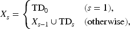
To evaluate the accuracy of the updated DNNs with respect to the past dataset, it is sufficient to test the DNNs with all the past data as input. In incremental learning, the size of the past dataset gradually increases, and then the time required to evaluate the change in accuracy with respect to the past dataset also increases. Until the test execution on the past dataset is completed, the DNN before or after the update is tentatively selected and used. If the operator does not have any information on the change in accuracy for the past dataset, the worst DNN may be selected. This results in undesirable business losses. Therefore, we propose a method to estimate the change in accuracy “fast” even if the past dataset is huge. This enables the operator to select a tentative DNN with consideration of the change in accuracy for the past dataset. As shown in Figure 2, by using the proposed method, the operator can make an early decision on DNN selection by referring to the estimated change of the updated DNN in terms of accuracy for the past dataset until the actual change is obtained by testing. This could enable better DNN operation and potentially reduce business losses.

Figure 2.

Usage of the proposed method. During the operation of deep neural network (DNN) $N_{s-1}$ , a new dataset is collected. By using this dataset, $N_{s-1}$ is trained and updated to $N_s$ . The operator tentatively selects whether to use $N_{s-1}$ or $N_s$ at the tentative decision point, and this decision can be reviewed at the final decision point from the test result of $N_s$ . Before the test execution of $N_s$ is completed, the proposed method provides the fast evaluation result of $N_s$ for the change in accuracy for the past dataset. This enables the operator to decide whether to continue using the tentatively selected DNN before the actual change in accuracy is obtained by testing at the final decision point. After $N_s$ is rigorously evaluated by testing, we can review the decision again.

The proposed method is useful for systems with the following characteristics. First, the external environment of the system, that is, the distribution of input values, gradually changes, and there are both micro and macro trends of change. Second, the system learns continuously from data streams and follows changes in its external environment. Examples of such systems are social infrastructure systems, such as weather prediction, power control, and so on. In the case of a system that forecasts electricity demand, even if there is a change in the past several weeks, it may be transient due to peculiar weather conditions. Therefore, the operator may be discouraged from updating the DNN if the accuracy for the past datasets is significantly decreased. Another example is a stock price forecasting system. Updating the DNN on the basis of micro trend changes could lead to significant business losses.

3. Proposed Method

3.1. Positive and Negative Gradients

It is supposed that DNN $N_s$ is developed by the $s$ th training on DNN $N_{s-1}$ . The DNN deals with a classification problem with class $c(c>1)$ . For any input value $x^m$ contained in $X_s$ , the corresponding expected output value $t(x^m)$ is given. Since the effect of the DNN update is evaluated for each classification class in the proposed method, we define $X_s^k\subseteq X_s$ as a set of input values with the same classification class $k$ . The purpose of the proposed method is to estimate the change in accuracy for $X_s^k$ when $N_{s-1}$ is updated to $N_s$ .

Consider the case where DNN $N_{s-1}$ fails in the inference for input value $x^m\in X_s^k$ , that is, $fst(\mathbf{y}(x^m))\ne t(x^m)$ . In this case, $x^m$ can be a factor that improves the accuracy of $N_{s-1}$ . When $N_{s-1}$ is updated to $N_s$ , if $N_s$ succeeds in the inference for $x^m$ , then the accuracy is increased. On the basis of this, we want to estimate how much the likelihood of successful inference for $x^m$ increases when updating DNN $N_{s-1}$ to $N_s$ . Therefore, in the proposed method, we focus on value changes of the c-dimensional vector $\mathbf{\text{y}}(x^m)=[y_1^m,\dots ,y_k^m,\dots ,y_c^m]$ . To avoid confusion between $\mathbf{\text{y}}(x^m)$ in $N_{s-1}$ and $\mathbf{\text{y}}(x^m)$ in $N_s$ , the output value of $N_{s-1}$ is hereafter described as $\mathbf{\text{y}}(x^m)=[y_1^m,\dots ,y_k^m,\dots ,y_c^m]$ and the output value of $N_s$ is $y^{\mathrm{\prime }}(x^m)=[y_1^{\mathrm{\prime }m},\dots ,y_k^{\mathrm{\prime }m},\dots ,y_c^{\mathrm{\prime }m}]$ .

If $N_{s-1}$ fails in the inference for $x^m$ , it means that $y_{t(x^m)}^m$ is not the largest in $\mathbf{\text{y}}(x^m)$ , that is, $y_{t(x^m)}^m<y_{fst(\mathbf{y}(x^m))}^m$ . Assume that the updated DNN $N_s$ infers the output value for $x^m$ successfully. In that case, $y_{t(x^m)}^{\mathrm{\prime }m}$ has increased or $y_{fst(\mathbf{y}(x^m))}^m$ has decreased so that $y_{t(x^m)}^{\mathrm{\prime }m}\ge y_{fst(\mathbf{y}(x^m))}^{\mathrm{\prime }m}$ holds. Therefore, we focus on the value change of $y_{t(x^m)}^m$ and $y_{fst(\mathbf{y}(x^m))}^m$ to estimate the likelihood of successfully inferring the output value for $x^m$ with $N_s$ . The more $y_{t(x^m)}^m$ increases, the more likely the output value for $x^m$ is successfully inferred. It is also true that the more $y_{fst(\mathbf{y}(x^m))}^m$ decreases, the more likely the output value for $x^m$ is successfully inferred. Note that $fst(\mathbf{y}(x^m))$ is the value with respect to $N_{s-1}$ . This means that $y_{fst(\mathbf{y}(x^m))}^{\mathrm{\prime }m}$ represents the value after $y_{fst(\mathbf{y}(x^m))}^m$ , the largest element value of $\mathbf{y}(x^m)$ , is changed by updating the DNN from $N_{s-1}$ to $N_s$ .

Similarly, consider the case where accuracy is decreased by updating the DNN. When the inference result of $x^m$ is changed from success to failure, that is, from $y_{t(x^m)}^m=y_{fst(\mathbf{y}(x^m))}^m$ to $y_{t(x^m)}^{\mathrm{\prime }m}\ne y_{fst(y^{\prime }(x^m))}^{\mathrm{\prime }m}$ . The factors that cause the accuracy to decrease are the values of $y_{fst(\mathbf{y}(x^m))}^m$ and $y_{fst(y^{\prime }(x^m))}^{\mathrm{\prime }m}$ . Here, $fst(y^{\prime }(x^m))$ denotes the class with the largest element value in $y^{\prime }(x^m)$ . Since the aim of this method is to estimate the effect on $X_s^k$ without running $N_s$ with $X_s^k$ including $x^m$ , it is assumed that $fst(y^{\prime }(x^m))$ is not known. Therefore, we use $snd(\mathbf{y}(x^m))$ instead of $fst(y^{\prime }(x^m))$ in the proposed method. This is based on the assumption that “If the inference result changes from success to failure when updating the DNN from $N_{s-1}$ to $N_s$ , the class with the largest probability in $N_s$ is likely to be that with the second largest probability in $N_{s-1}$ .” Here, since we assumed that $N_{s-1}$ succeeds in the inference for $x^m$ , the class with the largest probability in $N_{s-1}$ is $t(x^m)$ . If a class different from $t(x^m)$ has the largest value in $N_s$ , the class is highly likely to be $snd(\mathbf{y}(x^m))$ , the class with the second largest probability in $N_{s-1}$ , from the above assumption. Therefore, to estimate the possibility that $x^m$ fails in the inference after updating the DNN, we focus on changes in $y_{t(x^m)}^m$ and $y_{snd(\mathbf{y}(x^m))}^m$ . The more $y_{t(x^m)}^m$ decreases, the more likely inference for $x^m$ is to fail. It is also true that the more $y_{snd(\mathbf{y}(x^m))}^m$ increases, the more likely the inference for $x^m$ is to fail. The validity of the above assumption is experimentally evaluated in Appendix A.

In the proposed method, $X_s^k$ is input into $N_{s-1}$ and $N_{s-1}$ infers the output values before updating from $N_{s-1}$ to $N_s$ . The sets of input values that fail and succeed in the inference are denoted as $X_F\subseteq X_s^k$ and $X_T\subseteq X_s^k$ , respectively, where $X_F\cap X_T=\mathrm{\varnothing }$ . For simplicity, $X_T$ and $X_F$ are not given $s$ and $k$ as subscripts. For $x^m\in X_F$ , $fst(\mathbf{y}(x^m))\ne t(x^m)$ holds. Similarly, for $x^m\in X_T$ , $fst(\mathbf{y}(x^m))=t(x^m)$ holds.

For $x^m\in X_F$ , we define the positive loss $(\mathrm{PL})$ to evaluate the change in value of $y_{t(x^m)}^m$ and $y_{fst(\mathbf{y}(x^m))}^m$ , which cause an accuracy increase, as shown in Definition 2. Let $L$ be an arbitrary loss function used in the training. Assume that the first and second parameters of $L$ are the output value $\mathbf{y}(x^m)$ and the supervisory signal, respectively. If the DNN is updated so that $\mathrm{PL}$ decreases, the likelihood of a successful inference for $x^m\in X_F$ is increased. For $x^m\in X_T$ , we evaluate the value changes of $y_{t(x^m)}^m$ and $y_{snd(\mathbf{y}(x^m))}^m$ , which cause accuracy to decrease. We similarly define the negative loss $(\mathrm{NL})$ , as shown in Definition 2. If the DNN is updated so that $\mathrm{NL}$ decreases, it is more likely to fail in the inference for $x^m\in X_F$ .

Definition 2

$$\begin{array}{rl}\mathrm{PL}(x^m)& =L(\mathbf{y}(x^m),t(x^m))-L(\mathbf{y}(x^m),fst(\mathbf{y}(x^m))),\\ \mathrm{NL}(x^m)& =L(\mathbf{y}(x^m),snd(\mathbf{y}(x^m)))-L(\mathbf{y}(x^m),t(x^m)).\end{array}$$

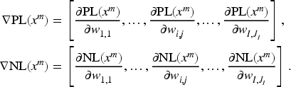
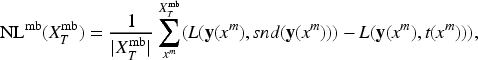
Next, we calculate the gradient of parameter $W_{s-1}=[w_{1,1},\dots ,w_{i,j},\dots ,w_{I,J_I}]$ of $N_{s-1}$ with respect to $\mathrm{PL}(x^m)$ . The gradient of $\mathrm{PL}(x^m)$ , called the positive gradient, is expressed by $\mathrm{\nabla }\mathrm{PL}(x^m)$ . Similarly, the gradient of $\mathrm{NL}(x^m)$ , called the negative gradient, is expressed by $\mathrm{\nabla }\mathrm{NL}(x^m)$ . $\mathrm{\nabla }\mathrm{PL}(x^m)$ and $\mathrm{\nabla }\mathrm{NL}(x^m)$ are defined as follows:

Definition 3

$$\begin{array}{rl}\mathrm{\nabla }\mathrm{PL}(x^m)& =[\frac{\mathrm{\partial }\mathrm{PL}(x^m)}{\mathrm{\partial }{w}_{1,1}},\dots ,\frac{\mathrm{\partial }\mathrm{PL}(x^m)}{\mathrm{\partial }{w}_{i,j}},\dots ,\frac{\mathrm{\partial }\mathrm{PL}(x^m)}{\mathrm{\partial }{w}_{I,J_I}}],\\ \mathrm{\nabla }\mathrm{NL}(x^m)& =[\frac{\mathrm{\partial }\mathrm{NL}(x^m)}{\mathrm{\partial }{w}_{1,1}},\dots ,\frac{\mathrm{\partial }\mathrm{NL}(x^m)}{\mathrm{\partial }{w}_{i,j}},\dots ,\frac{\mathrm{\partial }\mathrm{NL}(x^m)}{\mathrm{\partial }{w}_{I,J_I}}].\end{array}$$

3.2. Effect Estimation

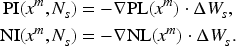
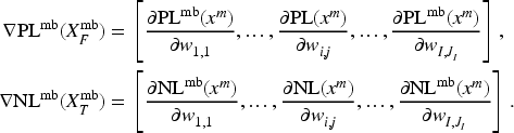
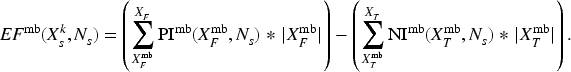
After $\mathrm{\nabla }\mathrm{PL}(x^m)$ and $\mathrm{\nabla }\mathrm{NL}(x^m)$ are created for $N_{s-1}$ , training $s$ is additionally executed, and DNN $N_s$ is created. Parameter $W_s$ of $N_s$ is compared with parameter $W_{s-1}$ of $N_{s-1}$ , and the update difference of parameter $\mathrm{\Delta }{W}_s=W_s-W_{s-1}$ is acquired. By using $\mathrm{\Delta }{W}_s$ , positive effect $\mathrm{PI}(x^m,N_s)$ and negative effect $\mathrm{NI}(x^m,N_s)$ to $x^m$ are calculated as follows:

Definition 4

$$\begin{array}{rl}\mathrm{PI}(x^m,N_s)& =-\mathrm{\nabla }\mathrm{PL}(x^m)\cdot \mathrm{\Delta }{W}_s,\\ \mathrm{NI}(x^m,N_s)& =-\mathrm{\nabla }\mathrm{NL}(x^m)\cdot \mathrm{\Delta }{W}_s.\end{array}$$

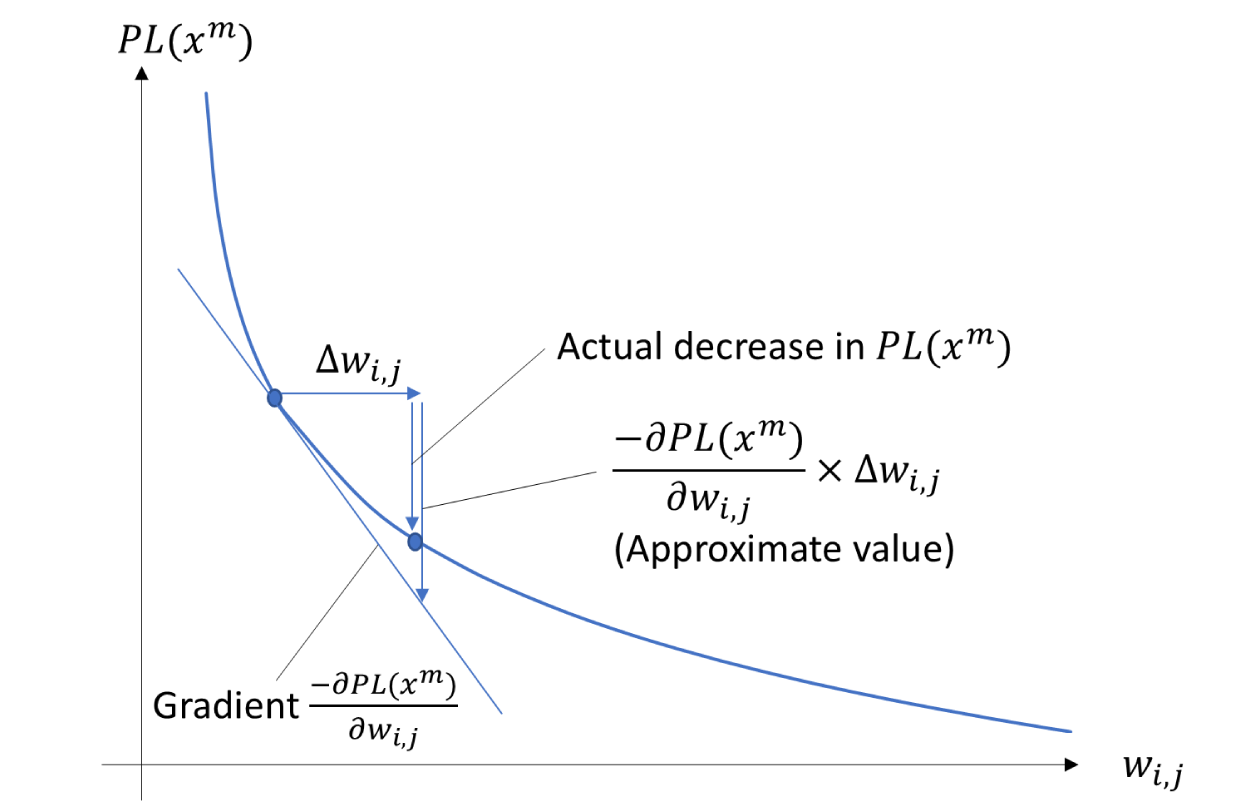
$\mathrm{PI}(x^m,N_s)$ approximates the amount by which $\mathrm{PL}(x^m)$ is decreased by updating parameter $W_{s-1}$ to $W_s$ . Likewise, $\mathrm{NI}(x^m,N_s)$ corresponds to the approximate decrease in $\mathrm{NL}(x^m)$ . If $\mathrm{\Delta }{W}_s$ is denoted as $[\mathrm{\Delta }{w}_{1,1},\dots ,\mathrm{\Delta }{w}_{i,j},\dots ,\mathrm{\Delta }{w}_{I,J_I}]$ , $\mathrm{PI}(x^m,N_s)$ corresponds to

$$\begin{array}{r}\sum _{i,j}(\frac{-\mathrm{\partial }\mathrm{PL}(x^m)}{\mathrm{\partial }{w}_{i,j}}\times \mathrm{\Delta }{w}_{i,j}).\end{array}$$

For example, in the case that loss function $L$ is cross-entropy, the relationship between the decrease in $\mathrm{PL}(x^m)$ due to updating $w_{i,j}$ by $\mathrm{\Delta }{w}_{i,j}$ , and its approximate value

$$\begin{array}{r}\frac{-\mathrm{\partial }\mathrm{PL}(x^m)}{\mathrm{\partial }{w}_{i,j}}\times \mathrm{\Delta }{w}_{i,j}\end{array}$$

is shown in Figure 3.

Figure 3.

Decrease in $\mathrm{PL}$ and its approximate value. When parameter $w_{i,j}$ increases by $\mathrm{\Delta }{w}_{i,j}$ , $\mathrm{PL}(x^m)$ decreases. Since the gradient of the loss function is $-\mathrm{\partial }\mathrm{PL}(x^m)/\mathrm{\partial }{w}_{i,j}$ , the change in $\mathrm{PL}(x^m)$ is approximated as $[-\mathrm{\partial }\mathrm{PL}(x^m)/\mathrm{\partial }{w}_{i,j}]\times \mathrm{\Delta }{w}_{i,j}$ .

We assume that the same loss function $L$ is used for training $N_s$ and $N_{s-1}$ . The training aims to reduce the loss calculated on the basis of $L$ (hereafter, training loss), in which the expected output value is the supervisory signal of the training. If the training loss for $x^m$ decreases, the output value of $N_s$ in regard to $x^m$ is more likely correct. This means that the decrease in training loss is a barometer for evaluating the change in accuracy. It can therefore be assumed that $\mathrm{PI}(x^m,N_s)$ , which is an approximate decrease in $\mathrm{PL}(x^m)$ , can be taken as a barometer for evaluating the change of the output value with respect to $x^m$ . More precisely, the decrease in $\mathrm{PL}(x_m)$ indicates the extent to which the likelihood of successfully inferring the output value for $x^m\in X_F$ is increased. This is also true for $\mathrm{NL}(x^m)$ . The decrease in $\mathrm{NL}(x_m)$ indicates the extent to which the likelihood of failing in inferring the correct output value for $x^m\in X_T$ is increased.

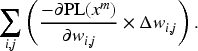
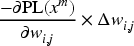
The sum of $\mathrm{PL}(x_m)$ for all $x^m\in X_F$ is the barometer of the accuracy increase in $X_F$ . Similarly, the sum of $\mathrm{NL}(x_m)$ for all $x^m\in X_T$ is a barometer of the accuracy decrease in $X_T$ . On the basis of the aforementioned considerations, the following $EF(X_s^k,N_s)$ in Definition 5 can be used as a barometer for evaluating the change in accuracy with respect to $X_s^k=X_F\cup X_T$ .

Definition 5

$$\begin{array}{r}EF(X_s^k,N_s)=\sum _{x^m}^{X_F}\mathrm{PI}(x^m,N_s)-\sum _{x^m}^{X_T}\mathrm{NI}(x^m,N_s).\end{array}$$

The purpose of the proposed method is to estimate the change in accuracy for the past dataset immediately after updating the DNN. To achieve this, we conduct some calculations in advance before updating the DNN, so that the amount of calculation after updating the DNN is minimized as much as possible. However, only formulas of Definitions 2 and 3 can be performed before the DNN is updated. Parameter $\mathrm{\Delta }{W}_s$ of the updated DNN $N_s$ is required for the calculation in Definition 4, so subsequent calculations can only be executed after updating the DNN. Moreover, since the computational complexity of the formulas in Definitions 4 and 5 depends on the number of input values contained in $X_s^k$ , the amount of calculations conducted after updating the DNN will increase as incremental learning progresses ( $X_s^k\subseteq X_s$ is increased as incremental learning progresses). Therefore, we replace the calculations in Definitions 4 and 5 with the following ones given in Definition 6 and Formula 1.

Definition 6

$$\begin{array}{r}\mathrm{GradSum}(X_s^k)=\sum _{x^m}^{X_F}(-\mathrm{\nabla }\mathrm{PL}(x^m))-\sum _{x^m}^{X_T}(-\mathrm{\nabla }NL(x^m)).\end{array}$$

Formula 1.

$$\begin{array}{r}EF(X_s^k,N_s)=\mathrm{GradSum}(X_s^k)\cdot \mathrm{\Delta }{W}_s.\end{array}$$

In Definition 4, $\mathrm{PI}(x^m,N_s)$ and $\mathrm{NI}(x^m,N_s)$ are created by multiplying $\mathrm{\nabla }\mathrm{PL}(x^m)$ and $\mathrm{\nabla }\mathrm{NL}(x^m)$ by $\mathrm{\Delta }{W}_s$ . After that, sum and subtraction calculations are conducted on them in Definition 5. To reduce the amount of calculations after updating the DNN, the sum and subtraction calculations are performed in Definition 6 before the DNN is updated. After the DNN is updated, $\mathrm{\Delta }{W}_s$ , which can only be obtained from the updated DNN $N_s$ , is multiplied in Formula 1. The computation time of Formula 1 is constant and independent of the number of input values contained in $X_s^k$ .

3.3. Regression Model

$EF$ can be used as a barometer to evaluate changes in accuracy. More specifically, $EF$ and accuracy are expected to have a linear relationship, which means that $EF$ increases and decreases along with accuracy. This relationship is expected regardless of the dataset. However, the scale of $EF$ values and the scale of accuracy values are different for each dataset. In other words, these scales depend on dataset type (i.e., the problem solved by the DNN) and DNN structure. Thus, there is no general way to estimate the change in accuracy from $EF$ . However, if we target a specific dataset and DNN, we are able to derive a formula regressionally from the actual calculation results of the $EF$ and the change in accuracy. Therefore, the proposed method creates a linear regression model to estimate the increase/decrease in accuracy from $EF$ .

First, we calculate $EF$ of DNN $N_1$ to $N_{s-1}$ for $X_s^k$ , that is, $EF(X_s^k,N_i)(1\le i\le s-1)$ , respectively. Also, by performing the inference of $N_0$ to $N_{s-1}$ with $X_s^k$ , respectively, the actual increase or decrease in accuracy with respect to $X_s^k$ is measured. By using these values of $EF(X_s^k,N_i)$ and the actual increase/decrease in accuracy, we create a linear regression model, where an $EF$ value is the input of the model and the increase/decrease in accuracy is the output. Note that the past dataset used for these calculations is $X_s^k$ because what we want to estimate at training $s$ is the effect of additional training $s$ on $X_s^k$ , not $X_i^k$ . The effect of $s$ on $X_s^k$ will be estimated on the basis of the actual effects of training 1 to $s-1$ on $X_s^k$ . Since $X_s^k$ is created from Dataset 0 to Dataset $s-1$ , it can be obtained at training $s-1$ . In other words, these calculations can be performed before training $s$ .

Next, the formulas of Definitions 2, 3, and 6 are performed, and $\mathrm{GradSum}(X_s^k)$ is obtained. These calculations can also be performed before training $s$ since $\mathrm{\Delta }{W}_s$ , which is the update difference of the parameters between $N_{s-1}$ and $N_s$ , is not used. After updating the DNN from $N_{s-1}$ to $N_s$ by training $s$ , $EF(X_s^k,N_s)$ is then calculated in accordance with Formula 1. $EF(X_s^k,N_s)$ is input to the linear regression model to estimate the value of the increase or decrease in accuracy with respect to $X_s^k$ due to the update from $N_{s-1}$ to $N_s$ . This enables us to estimate the effect on $X_s^k$ before executing the test of $N_s$ with $X_s^k$ .

The number of samples to create the linear regression model depends on the number of training $s$ . In the experiment shown in Section 4, the number of training is 100 ( $s=100$ ). We create the regression model using the results of training 1 to 99. When creating the regression model, the interquartile range (IQR) is calculated, and outliers are removed from the samples. In more detail, let IQR denote the interquartile range, $Q_1$ denote the lower quartile and $Q_3$ denote the upper quartile. Samples smaller than $Q_1-\mathrm{IQR}\times 1.5$ and larger than $Q_3+\mathrm{IQR}\times 1.5$ are removed as outliers. The samples larger than $Q_1-\mathrm{IQR}\times 1.5$ , and $Q_3+\mathrm{IQR}\times 1.5$ are also removed.

The amount of calculation of Formula 1, which is executed after training $s$ , depends on the number of elements of $W_s$ , not the number of input values contained in $X_s^k$ . For an MLP, the number of elements of $W_s$ is given as $O(I^2)$ for the number of neurons $I$ constituting the DNN. Moreover, the computational complexity of inference by the linear regression model is independent of $X_s^k$ and $W_s$ . Therefore, the calculation order of the proposed method after training $s$ is given as $O(I^2)$ . This means that even if $X_s^k$ is enormous, a change in accuracy can be evaluated in a short time.

3.4. Mini-Batch for PL and NL

The proposed method assumes that there is sufficient time between training $s-1$ and $s$ . More specifically, there is sufficient time to calculate $EF(X_s^k,N_i)$ for 1 $\le i\le s-1$ for creating a regression model, by executing DNNs $N_1$ to $N_{s-1}$ with $X_s^k$ to measure changes in accuracy, and to calculate $\mathrm{GradSum}(X_s^k)$ from the formulas in Definitions 2, 3, and 6. However, depending on the number of input values contained in $X_s^k$ , these calculations may not be finished. In particular, since the formulas in Definition 3 calculate the gradient for each input value $x^m$ , they require much time if $X_s^k$ is enormous. In such a case, positive and negative losses for mini-batch, denoted as ${\mathrm{PL}}^{\mathrm{mb}}$ and ${\mathrm{NL}}^{\mathrm{mb}}$ , respectively, are calculated as follows:

Definition 7

$$\begin{array}{r}{\mathrm{PL}}^{\mathrm{mb}}(X_F^{\mathrm{mb}})=\frac{1}{|X_F^{\mathrm{mb}}|}\sum _{x^m}^{X_F^{\mathrm{mb}}}(L(\mathbf{y}(x^m),t(x^m))-L(\mathbf{y}(x^m),fst(\mathbf{y}(x^m)))),\end{array}$$

$$\begin{array}{r}{\mathrm{NL}}^{\mathrm{mb}}(X_T^{\mathrm{mb}})=\frac{1}{|X_T^{\mathrm{mb}}|}\sum _{x^m}^{X_T^{\mathrm{mb}}}(L(\mathbf{y}(x^m),snd(\mathbf{y}(x^m)))-L(\mathbf{y}(x^m),t(x^m))),\end{array}$$

where $X_F^{\mathrm{mb}}$ and $X_T^{\mathrm{mb}}$ represent a mini-batch, and $X_F^{\mathrm{mb}}\subseteq X_F$ and $X_T^{\mathrm{mb}}\subseteq X_T$ hold. $|X_F^{\mathrm{mb}}|$ and $|X_T^{\mathrm{mb}}|$ denote the number of data contained in $X_F^{\mathrm{mb}}$ and $X_T^{\mathrm{mb}}$ , respectively.

Correspondingly, ${\mathrm{PI}}^{\mathrm{mb}}(X_F^{\mathrm{mb}})$ and ${\mathrm{NI}}^{\mathrm{mb}}(X_T^{\mathrm{mb}},N_s)$ are calculated from the gradient of ${\mathrm{PL}}^{\mathrm{mb}}(X_F^{\mathrm{mb}})$ and ${\mathrm{NL}}^{\mathrm{mb}}(X_T^{\mathrm{mb}})$ , and $\mathrm{\Delta }{W}_s$ , respectively, as shown in Definitions 8 and 9.

Definition 8

$$\begin{array}{rl}\mathrm{\nabla }{\mathrm{PL}}^{\mathrm{mb}}(X_F^{\mathrm{mb}})& =[\frac{\mathrm{\partial }{\mathrm{PL}}^{\mathrm{mb}}(x^m)}{\mathrm{\partial }{w}_{1,1}},\dots ,\frac{\mathrm{\partial }\mathrm{PL}(x^m)}{\mathrm{\partial }{w}_{i,j}},\dots ,\frac{\mathrm{\partial }{\mathrm{PL}}^{\mathrm{mb}}(x^m)}{\mathrm{\partial }{w}_{I,J_I}}],\\ \mathrm{\nabla }{\mathrm{NL}}^{\mathrm{mb}}(X_T^{\mathrm{mb}})& =[\frac{\mathrm{\partial }{\mathrm{NL}}^{\mathrm{mb}}(x^m)}{\mathrm{\partial }{w}_{1,1}},\dots ,\frac{\mathrm{\partial }\mathrm{NL}(x^m)}{\mathrm{\partial }{w}_{i,j}},\dots ,\frac{\mathrm{\partial }{\mathrm{NL}}^{\mathrm{mb}}(x^m)}{\mathrm{\partial }{w}_{I,J_I}}].\end{array}$$

Definition 9

$$\begin{array}{rl}{\mathrm{PI}}^{\mathrm{mb}}(X_F^{\mathrm{mb}},N_s)& =-\mathrm{\nabla }{\mathrm{PL}}^{\mathrm{mb}}(x^m)\cdot \mathrm{\Delta }{W}_s,\\ {\mathrm{NI}}^{\mathrm{mb}}(X_T^{\mathrm{mb}},N_s)& =-\mathrm{\nabla }{\mathrm{NL}}^{\mathrm{mb}}(x^m)\cdot \mathrm{\Delta }{W}_s.\end{array}$$

The larger mini-batch $X_F^{\mathrm{mb}}$ is, the more its inference results change from failure to success for more input values, so accuracy is likely to increase. Similarly, the larger mini-batch $X_T^{\mathrm{mb}}$ is, the more its inference results change from success to failure for more input values, so accuracy is likely to decrease. Thus, we calculate $E{F}^{\mathrm{mb}}$ by multiplying ${\mathrm{PI}}^{\mathrm{mb}}$ by $|X_F^{\mathrm{mb}}|$ and ${\mathrm{NI}}^{\mathrm{mb}}$ by $|X_T^{\mathrm{mb}}|$ , as shown in Definition 10.

Definition 10

$$\begin{array}{r}E{F}^{\mathrm{mb}}(X_s^k,N_s)=(\sum _{X_F^{\mathrm{mb}}}^{X_F}{\mathrm{PI}}^{\mathrm{mb}}(X_F^{\mathrm{mb}},N_s)*|X_F^{\mathrm{mb}}|)-(\sum _{X_T^{\mathrm{mb}}}^{X_T}{\mathrm{NI}}^{\mathrm{mb}}(X_T^{\mathrm{mb}},N_s)*|X_T^{\mathrm{mb}}|).\end{array}$$

Similar to the formulas of Definition 4, $\mathrm{\Delta }{W}_s$ appears in Definition 9, so it can only be executed after the DNN is updated. Since the computational complexities of Definitions 9 and 10 depend on the size of $X_s^k$ , the amount of calculation after the DNN update will increase as incremental learning proceeds. Therefore, just as the formulas of Definitions 4 and 5 were placed with Definition 6 and Formula 1, the formulas in Definitions 9 and 10 are placed with the following formulas in Definition 11 and Formula 2.

Definition 11

$$\begin{array}{r}{\mathrm{GradSum}}^{\mathrm{mb}}(X_s^k)=\sum _{X_F^{\mathrm{mb}}}^{X_F}(-\mathrm{\nabla }{\mathrm{PL}}^{\mathrm{mb}}(X_F^{\mathrm{mb}}))-\sum _{X_T^{\mathrm{mb}}}^{X_T}(-\mathrm{\nabla }{\mathrm{NL}}^{\mathrm{mb}}(X_T^{\mathrm{mb}})).\end{array}$$

Formula 2.

$$\begin{array}{r}E{F}^{\mathrm{mb}}(X_s^k,N_s)={\mathrm{GradSum}}^{\mathrm{mb}}(X_s^k)\cdot \mathrm{\Delta }{W}_s.\end{array}$$

4. Experiment

We experimentally applied the proposed method to the MNIST (Liu et al., 2003), Fashion MNIST (Xiao et al., 2017), and GTSRB (Stallkamp et al., 2011) datasets. In the following sections, arguments of the functions clear from the context have been omitted.

4.1. Setup

In this experiment, trainings are conducted from $s=0$ to $100$ . Two-thirds of the entire dataset is used as Dataset 0 (see Figure 1). The remaining is divided equally to create Datasets 1 through 100. In incremental learning, a well-learned model is continuously updated, so if Dataset 0 is too small and then DNN $N_0$ is not sufficiently trained, an appropriate simulation of incremental learning cannot be performed. On the other hand, if Datasets 1 to 100 are too small, problems such as overfitting may occur. Based on our system development experiences, we believe that the system will never be launched with the initial DNN $N_0$ that is not trained sufficiently. From the above consideration, we decided to prioritize Dataset 0 and made it from two-thirds of the entire dataset. For example, for the MNIST dataset, which contains 70,000 image data, 46,666 data are designated as Dataset 0, and Datasets 1 through 100 each consist of approximately 233 data. The ratio of dividing each dataset into the training and test datasets should be the same as the ratio of the training to test datasets in the original dataset. For the MNIST dataset, 60,000 and 10,000 data are provided for the training and testing datasets, respectively, resulting in a split ratio of $6:1$ .

As for the DNN models, we use an MLP with one hidden layer (composed of 1,000 neurons) in addition to the input and output layers and a convolutional neural network (CNN) with two convolutional layers with a kernel size of $3\times 3$ and a stride size of 1. For the GTSRB dataset, we use the mini-batch method described in Section 3.4 because the images (color channels) are too large to calculate the gradient for every input value in accordance with the formulas in Definition 3. In this experiment, the size of the mini-batch is set to 50.

We assume that we have finished training 100 and obtained DNN $N_{100}$ . Before that, past dataset $X_{100}^k$ was created from Datasets 0 to 99, and then $EF(X_{100}^k,N_i)(1\le i\le 99)$ were calculated. In addition, the actual increases or decreases in accuracy for $N_1$ to $N_{99}$ were also calculated by running $N_0$ to $N_{99}$ with $X_{100}^k$ as the input. By using these data as samples, a linear regression model was created before training 100. After finishing training 100, we can calculate $EF(X_{100}^k,N_{100})$ by comparing DNN $N_{99}$ and $N_{100}$ . By inputting $EF(X_{100}^k,N_{100})$ into the linear regression model, the change in accuracy at training 100 is estimated. Therefore, the proposed method can be evaluated by the performance of the regression model.

If possible, we want to calculate the coefficient of determination for the created regression model with test data. However, the test data to evaluate the created regression model cannot be sufficiently obtained since only the data to evaluate the regression model is that from training 100. Even if training 101 is conducted subsequently, the target dataset $X_{100}^k$ will be updated to $X_{101}^k$ , and thus a different regression model will be created at training 101. This means that only one data is used as input for each regression model. Therefore, for the evaluation of the proposed method, we calculate the $R^2$ score of the regression model at training 100 using the data of training 1 to 99 that are used to create the regression model. If the $R^2$ score is high, the regression estimation performance for the data from training 1 to 99 is also high. Furthermore, we can say that the estimation performance for the data of training 100 should be high since it is calculated in the same way as that from trainings 1 to 99.

In each training, cross-entropy is used as the loss function $L$ . The experiment was performed on an Ubuntu 20.04.4 LTS machine equipped with two Intel® Xeon® Gold 6132 2.6-GHz processors with 14 cores, 786-GB memory. It also has eight NVIDIA® Tesla®V100 NVLink GPUs.

4.2. Results

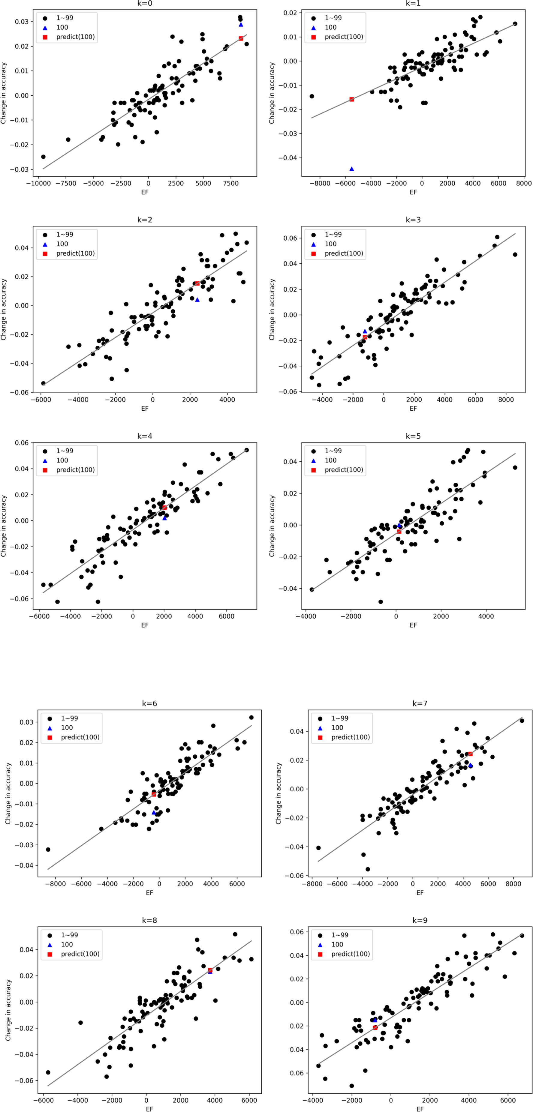
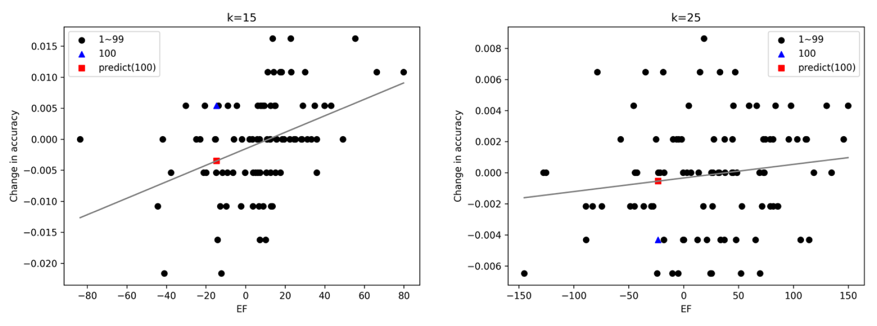
For the MNIST dataset, the linear regression model of the MLP resulting from the experiment is shown in Figure 4. The x- and y-axes show the values of $EF$ and the change in accuracy between before and after training 100, respectively.

Figure 4.

(1/2) Regression models of the MLP for the MNIST dataset. Each graph represents the result of applying the proposed method to each classification class. The x- and y-axes show the values of $EF$ and the change in accuracy between before and after training 100. The black dots are plotted from the values of $EF$ calculated by the proposed method and the actual change in accuracy in training 1 to 99. They are used to create the regression models, which are represented by straight black lines. The blue triangles represent the accuracy change estimated by the proposed method in training 100. The red rectangles represent the actual accuracy change in training 100, calculated by executing the DNN with all input values included in $X_{100}^k$ . (2/2). Note. MLP = multilayer perceptron; DNN = deep neural network.

The black dots in Figure 4 represent the data from trainings 1 to 99 used to create the regression model. However, outliers excluded on the basis of the IQR are not shown. The blue triangles represent the accuracy change estimated by the proposed method in training 100. The red rectangles represent the actual accuracy change in training 100, calculated by executing the DNN with all input values included in $X_{100}^k$ . The results for the other datasets were generally similar, with a few exceptions. Cases where the results were not as expected are discussed in Section 5.

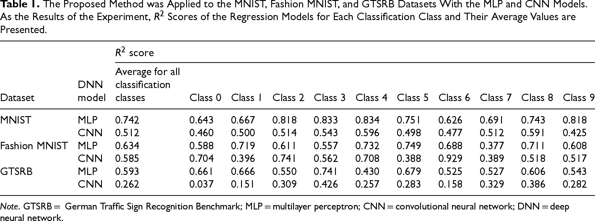
The $R^2$ scores of the linear regression models created for the MNIST, Fashion MNIST, and GTSRB datasets are shown in Table 1. Only $R^2$ scores for classification classes 0 through 9 are shown. For the GTSRB dataset, the column “Average for all classification classes” shows the average of all 43 classes. These results are discussed in Section 5.

Table 1.

The Proposed Method was Applied to the MNIST, Fashion MNIST, and GTSRB Datasets With the MLP and CNN Models. As the Results of the Experiment, $R^2$ Scores of the Regression Models for Each Classification Class and Their Average Values are Presented.

		$R^2$ score
		Average for all
	DNN	classification
Dataset	model	classes	Class 0	Class 1	Class 2	Class 3	Class 4	Class 5	Class 6	Class 7	Class 8	Class 9
MNIST	MLP	0.742	0.643	0.667	0.818	0.833	0.834	0.751	0.626	0.691	0.743	0.818
	CNN	0.512	0.460	0.500	0.514	0.543	0.596	0.498	0.477	0.512	0.591	0.425
Fashion MNIST	MLP	0.634	0.588	0.719	0.611	0.557	0.732	0.749	0.688	0.377	0.711	0.608
	CNN	0.585	0.704	0.396	0.741	0.562	0.708	0.388	0.929	0.389	0.518	0.517
GTSRB	MLP	0.593	0.661	0.666	0.550	0.741	0.430	0.679	0.525	0.527	0.606	0.543
	CNN	0.262	0.037	0.151	0.309	0.426	0.257	0.283	0.158	0.329	0.386	0.282

Note. GTSRB =  German Traffic Sign Recognition Benchmark; MLP = multilayer perceptron; CNN = convolutional neural network; DNN = deep neural network.

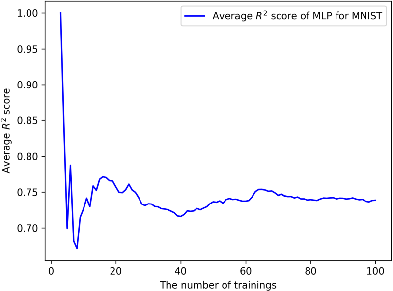
In training 3 to 99, the proposed method can also be applied to estimate each change in accuracy. Since at least two samples are required to create a linear regression model, the proposed method can be applied when the number of training $s$ is three or more. We conducted an additional experiment applying the proposed method to the MLP for the MNIST dataset in training 3 to 99. Figure 5 shows the average $R^2$ scores of the MLP from training 3 to 100 for the MNIST dataset. When the number of training is small, the number of data used to create the regression model is also small. As described in Section 4.1, $R^2$ scores are calculated from the data that are used to create the regression model since we have only one data for each training to evaluate the regression model. If these data can be connected by a straight line, the $R^2$ score is likely to be high. If they are scattered, the regression model is created at the center of the data, so the $R^2$ score is likely to be low. For example, in training $s=3$ , $EF(X_3^k,N_1)$ , $EF(X_3^k,N_2)$ (and their corresponding actual changes in accuracy) are used to create a regression model. These two data are also used to calculate the $R^2$ score. Since the regression model is formed as a line connecting these two data points, the $R^2$ score is 1. From around training 20, the $R^2$ score generally remained at 0.75 in Figure 5. This suggests that the proposed method is useful from the early stages of incremental learning.

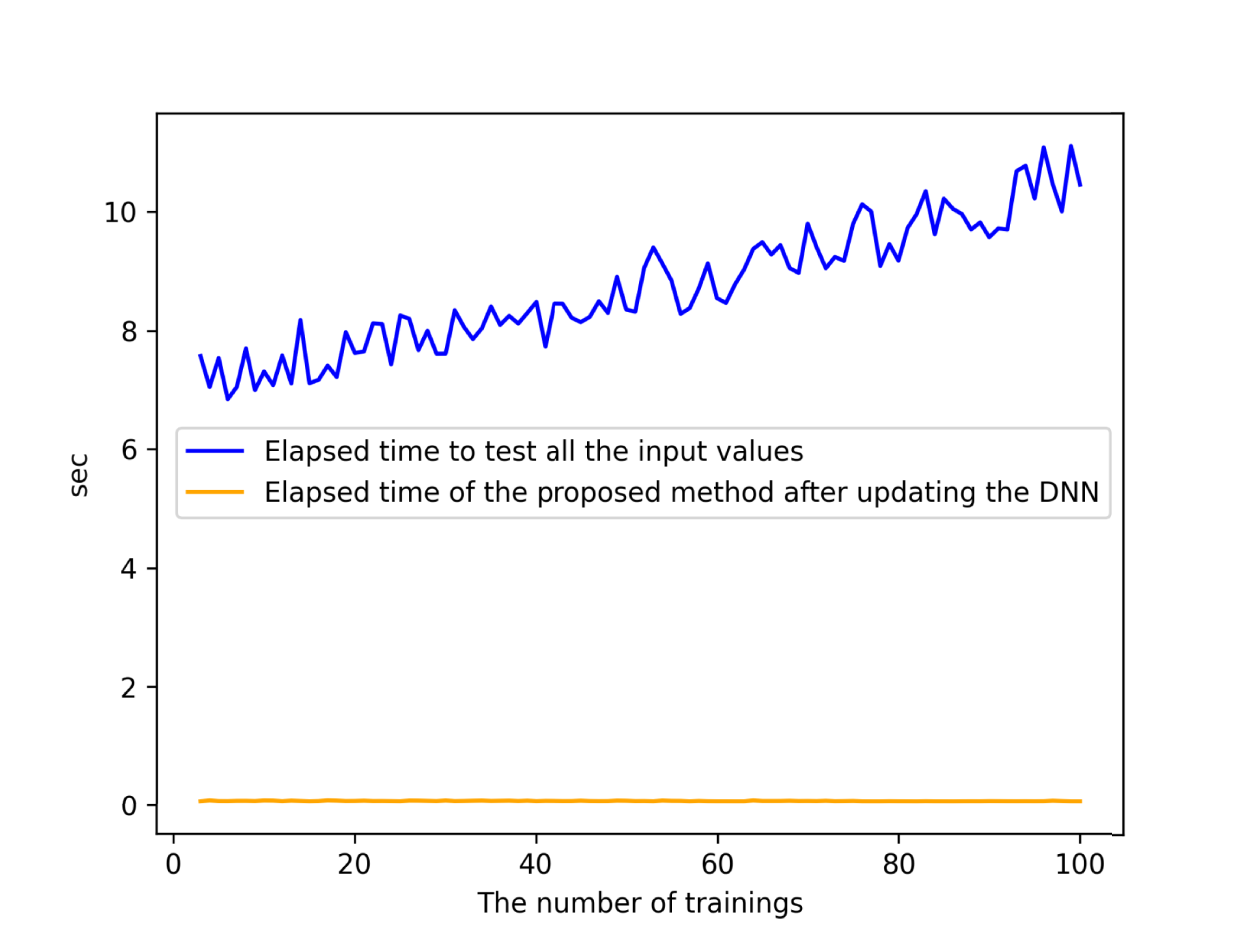
The time taken after updating the DNN, which is the MLP for the MNIST dataset, in the proposed method and that taken to test the DNN with all input values contained in $X_s$ for $s=3,4,\dots ,100$ are plotted in Figure 6. In the proposed method, the calculations conducted after updating the DNN are to obtain $EF$ from $\mathrm{GradSum}$ in accordance with Formula 1 and the value of increase or decrease in accuracy by inputting the value of $EF$ into the regression model. $\mathrm{PL}/\mathrm{NL}$ , $\mathrm{\nabla }\mathrm{PL}/\mathrm{\nabla }\mathrm{NL}$ , and $\mathrm{GradSum}$ are calculated before updating the DNN, so they are not included in the time shown in Figure 6. Figure 6 indicates that the calculation after updating the DNN can be performed in almost the same time regardless of the increase in the number of input values (orange line). In contrast, the test execution time increases with the number of training since the number of input values in $X_s$ increases (blue line). Similar results were obtained for the other datasets.

As shown in Figure 6, in the proposed method, the calculation after updating the DNN does not depend on the number of input values in the past dataset. The larger the past dataset is, the more useful the proposed method is to obtain reference information for tentatively selecting a DNN until the accurate change in accuracy is confirmed by test execution. It is evident that the calculation order of Formula 1, which is performed after updating the DNN, is $O(I^2)$ for each classification class as mentioned in Section 3.3. The amount of calculations corresponding to the formulas in Definitions 2, 3, and 6 increases in accordance with the size of the past dataset, but those calculations are carried out before the DNN is updated. This means that after the DNN is updated, the proposed method can estimate the change in accuracy in a constant time, even if the number of data included in the past dataset is enormous. However, the proposed method is useful only when the past dataset is not small. For example, in Figure 6, about 10,000 input values of the MNIST dataset are inferred in training 100, which takes only about 10 s. If the proposed method is used for tentatively selecting DNNs as described in Section 2.3, the shorter the time until the accurate change in accuracy is confirmed by testing, the less useful the proposed method will be. Assuming that the proposed method is effective if it takes more than 1 h to confirm the accurate change in accuracy, the past dataset should contain more than 3 million input values, as calculated from the results in Figure 6.

Figure 5.

Average $R^2$ scores in trainings 3 to 100 when the proposed method is applied to the multilayer perceptron (MLP) for the MNIST dataset. The x- and y-axes show the number of trainings and the average $R^2$ score, respectively.

Figure 6.

Calculation times in training $s=3$ to $100$ when the proposed method is applied to the MLP for the MNIST dataset. The yellow line represents the times taken after updating the DNN in the proposed method. The blue line represents the times taken to test the DNN with all input values contained in $X_s$ . Note. MLP = multilayer perceptron; DNN = deep neural network.

5. Evaluation and Discussion

5.1. Validity of the Evaluation

As mentioned in Section 4.1, the $R^2$ score shown in Table 1 is calculated using the data used to create the regression model. $X_s^k$ is updated each time the number of training increases. Hence, in the proposed method, the regression model is recreated for each training. That is, in training $s$ , the regression model is only used to estimate the change in accuracy for $X_s^k$ when the DNN is updated from $N_{s-1}$ to $N_s$ and is not used thereafter. In other words, the only data that can be used to evaluate the regression model is the data of training $s$ , but one data is not sufficient for evaluation. Therefore, the $R^2$ score calculated from the data of training 1 to $s-1$ is used to evaluate the regression models alternatively. These data are calculated from a DNN with the same structure and dataset $X_s^k$ as the data of training $s$ . Therefore, it can be used to evaluate the performance of the regression model. For example, suppose that the residuals between the data of training $t(1\le t\le s-1)$ and the regression model are small. This means that the regression model can accurately estimate the effect of the DNN updates in training $t$ for the dataset $X_s^k$ . If the same is generally true for any $t$ , then it is highly likely that the same regression model can accurately estimate the effect of DNN updates in training $s$ for the same dataset $X_s^k$ . On the basis of the aforementioned consideration, we used the data of training 1 to $s-1$ for the evaluation.

5.2. Performance

From the results of the experiment shown in Table 1, we found that the average $R^2$ score is around 0.6, which indicates that the proposed method can be expected to perform at a certain level. In particular, using the proposed method is preferable if the purpose is to obtain reference information for selecting a tentative DNN, as described in Section 2.3. The results of the experiment also show that the proposed method does not always estimate accurately. As shown in Table 1, the $R^2$ scores of the regression models can be around 0.1 if they are low. The limitations of the proposed method should be taken into consideration when using it.

In a number of cases, especially for the CNN with the GTSRB dataset, the linear relationship between $EF$ and accuracy change could not be confirmed. As examples, linear regression models for the GTSRB dataset with classification class $k=15$ and $25$ are shown in Figure 7. In these cases, the accuracy change is difficult to estimate by the proposed method. One common point among these cases is that the accuracy changes on the y-axis are smaller than those in Figure 4. This means that the inference results do not change significantly for most input values. In this case, the correlation between $EF$ and the change in accuracy should be low.

Figure 7.

Regression models of the CNN for classification class $k=15$ and $25$ of GTSRB dataset. These are examples of cases where the accuracy change is difficult to estimate by the proposed method. As in Figure 4, the x- and y-axes show the values of $EF$ and the change in accuracy between before and after training 100. The black dots are plotted from the values of $EF$ calculated by the proposed method and the actual change in accuracy in training 1 to 99. They are used to create the regression models, which are represented by straight black lines. The blue triangles represent the accuracy change estimated by the proposed method in training 100. The red rectangles represent the actual accuracy change in training 100, calculated by executing the DNN with all input values included in $X_{100}^k$ . Note. CNN = convolutional neural network; GTSRB = German Traffic Sign Recognition Benchmark; DNN = deep neural network.

When DNN $N_{s-1}$ before being updated succeeds in the inference (i.e., $fst(\mathbf{y}(x^m))=t(x^m)$ ) for many $x^m\in X_s^k$ but there is a large difference between the values of $y_{fst(y(x^m))}^m$ and $y_{snd(\mathbf{y}(x^m))}^m$ , the inference results do not change even though $\mathrm{PI}$ and $\mathrm{NI}$ change. In this case, since the number of input values in $X_F$ is small, the sum of $\mathrm{PI}$ will slightly change. For the same reason, accuracy will be unlikely to increase. However, since the number of input values contained in $X_T$ is large, the sum of $\mathrm{NI}$ is likely to increase significantly. According to the definition of $\mathrm{NL}$ (in Definition 2), when $y_{fst(\mathbf{y}(x^m))}^m$ decreases or $y_{snd(\mathbf{y}(x^m))}^m$ increases, $\mathrm{NI}$ increases. If there is a large difference between those values, the value of $y_{fst(\mathbf{y}(x^m))}^m$ is seldom smaller than that of $y_{snd(\mathbf{y}(x^m))}^m$ . That is, even if the value of $\mathrm{NI}$ increases, the relationship $y_{fst(\mathbf{y}(x^m))}^m>y_{snd(\mathbf{y}(x^m))}^m$ is likely to remain true, and then accuracy will not decrease. Thus, the closer the value of $\mathbf{y}(x^m)$ is to $t(x^m)$ (one-hot representation of $t(x^m)$ in reality) for most input values, the smaller the change in accuracy becomes. This determines whether the proposed method can accurately estimate the change in accuracy.

5.3. Application to Each Classification Class

The proposed method is applied to each classification class $k$ . We realized from experiments other than those described in Section 4 that when the proposed method is applied to $X_s$ , the $R^2$ score of the regression model is lower than in the cases of $X_s^k$ . In the proposed method, $\mathrm{PL}$ and $\mathrm{NL}$ are defined on the basis of the probability values of $\mathbf{y}(x^m)$ that change the inference result. The gradients of $\mathrm{PL}$ and $\mathrm{NL}$ are then calculated using the parameters of the DNN, and $\mathrm{PI}$ and $\mathrm{NI}$ are the results of evaluating the similarity with the actual DNN parameter change values $\mathrm{\Delta }{W}_s$ . These values represent the extent to which changes of the parameters cause “changes in probability values that affect the inference result.” Since $EF$ is calculated from the $\mathrm{PI}$ and $\mathrm{NI}$ of all input values, it represents the sum of the change in the probability values for each input value that affects the inference result.

Here, we note that input values in the same classification class are similar in terms of not only the probability value but also the amount of change in the probability value that flips the inference result from failure to success or vice versa. For example, for a dataset consisting of input values in the same classification class, the value of $EF$ that flips the inference result of an input value is assumed to be 5. Let us assume that the dataset consists of five input values, and the value calculated as the sum of the $EF$ values of those input values is 10. There can be three typical cases: $EF$ value of 2 from all 5 input values, $EF$ values of 10 from only 1 input value, and $EF$ values of 5 from 2 input values. In each case, the number of input values whose inference result flips is 0, 1, and 2, respectively. That is, when (the sum of) $EF$ is 10, the number of input values whose inference result flips can be estimated to be from 0 to 2.

Next, consider the case where input values of different classification classes are mixed. In this case, the values of $EF$ that would flip the inference result are different for each input value. Suppose that if the dataset consists of the five input values, the values of $EF$ that flip the inference result are 1, 1, 3, 3, 10 for each respective input value. It is also supposed that the value calculated as the sum of $EF$ values of those input values is 10. In this case, the number of input values whose inference result flips could be any number from 0 to 4. In other words, in this case, we can only narrow down that the number of input values whose inference result flips to be between 0 and 4 when $EF$ is 10. Thus, when input values of different classification classes are mixed, it is more difficult to narrow down the number of input values for which the inference result flips from $EF$ than when only input values of the same classification class are included. This means that the correlation between $EF$ and accuracy changes will be lower for a mixed dataset. For this reason, the proposed method is designed to be applied to each classification class.

We also realized from another experiment that applying the mini-batch method does not significantly change the $R^2$ score. This can also be explained by the fact that input values in the same classification class have similar features. If a mini-batch $X^{\mathrm{mb}}$ was composed of various input values $x^m$ with different characteristics, positive losses $\mathrm{PL}(x^m)$ were expected to be diverse. Since $\mathrm{PL}(X^{\mathrm{mb}})$ is calculated as the average of $\mathrm{PL}(x^m)$ , $\mathrm{PL}(x^m)$ and $\mathrm{PL}(X^{\mathrm{mb}})$ are not similar for many $x^m$ in this case. However, mini-batches $X^{\mathrm{mb}}$ consist of input values from the same classification class, and their inference results are the same. Therefore, the $\mathrm{PL}(x^m)$ calculated for each $x^m$ are all similar functions. Moreover, their average, $\mathrm{PL}(X^{\mathrm{mb}})$ , is also similar to $\mathrm{PL}(x^m)$ . From these considerations, the value obtained by calculating $\mathrm{PI}$ for each $x^m$ and summing them is highly likely to be similar to the value obtained by calculating $\mathrm{PI}$ for each mini-batch $X^{\mathrm{mb}}$ and multiplying it by the number of its elements $|X^{\mathrm{mb}}|$ . In other words, when the proposed method is applied to each classification class, the mini-batch method is likely to provide a similar result to the normal method. In fact, when we experimented with varying the number of input values that make up the mini-batch, no significant change in $R^2$ scores was observed.

$\mathrm{PL}(x^m)$ is calculated for each input value $x^m$ included in the mini-batch $X_F^{\mathrm{mb}}$ and the average value is used as $\mathrm{PL}(X_F^{\mathrm{mb}})$ . The gradient $\mathrm{\nabla }\mathrm{PL}(X_F^{\mathrm{mb}})$ is obtained for this average value. The gradient indicates how to update the parameters of the DNN so that it has a good (changing from failure to success) impact on average on the inference results of the input values contained in the mini-batch. It is used to compute the impact (i.e., $EF$ ) on the entire mini-batch by comparing it with the update of the DNN parameters. On the other hand, in the normal method, the gradient $\mathrm{\nabla }\mathrm{PL}(x^m)$ indicates how to update the parameters so that it positively impacts that input value. Recalling that the change in accuracy is the accumulation of the change in inference results for individual input values, the impact of the DNN update on individual input values is considered to have a higher correlation with the change in accuracy than the average impact on the mini-batch. For example, suppose that $\mathrm{\nabla }\mathrm{PL}(x^1)=\alpha$ and $\mathrm{\nabla }\mathrm{PL}(x^2)=-\alpha$ for a mini-batch consisting of $x^1$ and $x^2$ . It is also assumed that the parameters of the DNN are updated in the direction that $\mathrm{PL}(x^1)$ decreases. In that case, since $\mathrm{PL}(x^2)$ increases, the inference result for $x^2$ remains a failure. On the other hand, since $\mathrm{PL}(x^1)$ decreases, the inference result for $x^1$ is likely to change from failure to success, which may result in an increase in accuracy. However, if the mini-batch method is applied, since $\mathrm{\nabla }\mathrm{PL}(X_F^{\mathrm{mb}})=\alpha -\alpha =0$ , the value of $\mathrm{PL}(X_F^{\mathrm{mb}})$ does not change, that is, $\mathrm{PI}(X_F^{\mathrm{mb}},N_s)=0$ even though $\mathrm{PL}(x^1)$ decreases. Thus, the application of the mini-batch method can be a factor that reduces the correlation between $\mathrm{PI}$ and changes in accuracy. The same is true with $\mathrm{NL}$ . Therefore, the $R^2$ score of the linear regression model is likely to be lower when the mini-batch method is applied.

In the calculations of $\mathrm{PL}$ and $\mathrm{NL}$ , not only $t(x^m)$ but also $fst(\mathbf{y}(x^m))$ and $snd(\mathbf{y}(x^m))$ are used, respectively. This is because we expect to use cross-entropy as the loss function $L$ . Cross-entropy uses only the probability value of a particular classification class given as a supervisory signal. Therefore, for $\mathrm{PL}$ , calculating the loss on the basis of only $t(x^m)$ as the supervisory signal would only consider how much the value of $y_{t(x^m)}^m$ increases. This means that the loss does not include how much the value of $y_{fst(\mathbf{y}(x^m))}^m$ decreases. Similarly, for $\mathrm{NL}$ , if only $t(x^m)$ is given as the supervisory signal and the loss is calculated on the basis of it, only the amount by which the value of $y_{t(x^m)}^m$ decreases is taken into account. The loss does not include the amount by which the value of $y_{snd(\mathbf{y}(x^m))}^m$ increases. Therefore, the proposed method defines the calculations of $\mathrm{PL}$ and $\mathrm{NL}$ so that the values of $y_{t(x^m)}^m$ , $y_{fst(\mathbf{y}(x^m))}^m$ , and $y_{snd(\mathbf{y}(x^m))}^m$ are considered as factors affecting the change in accuracy. The mean squared error is calculated using probability values other than the class given as the supervisory signal. Therefore, if it is used as the loss function, terms in which $fst(\mathbf{y}(x^m))$ and $snd(\mathbf{y}(x^m))$ appear may be able to be removed from the formulas calculating $\mathrm{PL}$ and $\mathrm{NL}$ , respectively.

In the experiments described in Section 4, the original dataset was randomly split, so the distribution of the data did not change during incremental learning. This means that the effectiveness of the proposed method for concept drift was not evaluated. However, since the objective of the incremental learning shown in Section 2.2 is to adapt the DNN to concept drift as fast as possible, the DNN is assumed to be updated at a higher frequency than the frequency at which concept drift occurs. Hence, in many cases, the DNN will be updated even though concept drift has not occurred. Evaluating the effectiveness of the proposed method even when concept drift occurs is a future task.

6. Related Work

To the authors’ knowledge, no research on a method for the fast evaluation of incremental learning results has been published. However, there are several works on incremental learning that focus on the parameters of DNNs (weights and biases) and the gradient of a loss function.

Kirkpatrick et al. (2017) focused on a decrease in accuracy in task-incremental learning (Parisotto et al., 2015; Rusu et al., 2015). For example, when training for task 2 is carried out after training for task 1, the performance of the previously trained task (task 1) is catastrophically reduced. This is called catastrophic forgetting (Aleixo et al., 2023; Kemker et al., 2018; McCloskey & Cohen, 1989; McRae & Hetherington, 1993; Ratcliff, 1990). In response to this problem, they proposed a method of identifying the parameters important in regard to task 1, and training task 2 in a manner that minimizes changes to those parameters (important in regard to task 1). Our proposed method does not distinguish the parameters of the DNN. The accuracy change may be able to be estimated more accurately by identifying the parameters that contribute to the accuracy change for the dataset and focusing on the changes in those parameters, as in their method.

In task-incremental learning and class-incremental learning, distillation loss is used to mitigate catastrophic forgetting (Aljundi et al., 2017; Castro et al., 2018; Dhar et al., 2019; Douillard et al., 2020; Hou et al., 2018, 2019, 2019?; Kang et al., 2022; Li & Hoiem, 2017; Liu et al., 2020; Rannen et al., 2017; Rebuffi et al., 2017; Wu et al., 2019). Distillation loss represents the difference between the inference results before and after learning. The more similar the inference results, the smaller the distillation loss value. Learning to minimize distillation loss in addition to the normal loss enables inference results for the past dataset to be preserved. Kang et al. (2022) proposed a learning method that focuses on the gradient of the loss function. In this method, learning is performed so that “the increase in the loss” for the past dataset when the DNN is updated is minimized. To achieve this, they focus on the gradient of the loss function for the past dataset. On the basis of this gradient, the change in loss for the past dataset is approximated, and the DNN is updated so that it is minimized. In our proposed method, $\mathrm{PL}$ and $\mathrm{NL}$ are defined for the past dataset, and the impact of DNN update on the past dataset is estimated on the basis of their gradients. From a general point of view, our method and Kang et al.’s (2022) method are similar in that they focus on the gradient of the loss function for the past dataset and estimate the impact of the DNN update on the basis of the gradient. Unlike their method, however, our proposed method aims to estimate the change in accuracy for the past dataset. For this purpose, we propose $\mathrm{PL}$ and $\mathrm{NL}$ , which are directly related to the change in accuracy, rather than the normal loss.

In another approach, Belouadah et al. (2020) focused on the fact that the weights of a DNN before the update represent the past classes in class-incremental learning. Their method, which uses the weights to prevent catastrophic forgetting, is effective for memoryless class-incremental learning where the past dataset cannot be stored entirely. Our proposed method also utilizes the change in weight before and after DNN update, which is similar to their approach. However, our method cannot be applied to memoryless class-incremental learning since we cannot evaluate the accuracy for a past dataset without it. Although the proposed method can be applied to part of the past dataset, its accuracy estimation is expected to be lower.

7. Conclusion

We proposed a fast evaluation method for the effect of additional training for the past dataset in incremental learning. The gradient of the parameter values for the past dataset is extracted by running the DNN before the additional training. After the training, a barometer of the effect on the accuracy with respect to the past dataset is calculated from the gradient and update differences of the parameter values. Finally, the proposed method estimates the change in accuracy by using a regression model created from the $EF$ s and actual changes in accuracy in the past training. The computational complexity of the proposed method, after the update, depends on the number of DNN parameters, not on the amount of data in the past dataset. Therefore, even if the amount of data included in the past dataset is enormous, applying the proposed method enables the effects of training to be evaluated fast. When a DNN is updated during operation, the proposed method enables a system operator to decide whether to use the updated DNN with consideration of the change in accuracy for the past dataset. The results of our experiments indicate the usefulness of the proposed method in terms of computation time and the coefficient of determination for the regression model used to estimate changes in accuracy. Even though the expected coefficient of determination could not be confirmed in a number of cases, using the proposed method to obtain reference information for selecting a tentative DNN is preferable until an accurate change in accuracy is confirmed by test execution. As for future work, the proposed method will be more elaborately evaluated using other datasets. In particular, the occurrence of concept drift should be simulated in the evaluation. Moreover, improving the means of creating $EF$ will help in the search for a way to more accurately evaluate the change in accuracy. For example, distillation loss discussed in Section 6 may be effective for improving the proposed method.