How to Exhibit More Predictable Behaviors

Abstract

This paper looks at predictability problems, that is, wherein an agent must choose its strategy in order to optimize the predictions that an external observer could make. We address these problems while taking into account uncertainties in the environment dynamics and the observed agent’s policy. To that end, we assume that the observer (1) seeks to predict the agent’s future action or state at each time step, and (2) models the agent using a stochastic policy computed from a known underlying problem, and we leverage on the framework of observer-aware Markov decision processes (OAMDPs). We design reward functions for the agent which encode her goal to make next states or actions predictable by the observer; show that these induced predictable OAMDPs can be represented by goal-oriented or discounted MDPs; and analyze the properties of the proposed reward functions theoretically. Experiments have been conducted, generating and interpreting policies on two types of grid-world problems, and then confronting human observers to these policies on some of these problems.

1. Introduction

In a human–agent collaboration scenario, some properties of the agent behavior can be useful for the human and sometimes allow a better collaboration. Recent papers suggest ways of obtaining such behaviors. In particular, when an agent is aware that it is being observed by a passive human, as in Figure 1, it can control the information disclosed to the observer through its behavior.

Chakraborti et al. (2019) build on previous work to derive a taxonomy of these concepts. In particular, they distinguish between (1) transmitting information, with properties such as legibility (legible behaviors convey intentions, that is, actual task at hand, via action choices), explicability (explicable behaviors conform to observers’ expectations, that is, they appear to have some purpose), and predictability (a behavior is predictable if it is easy to guess the end of an on-going trajectory); or (2) hiding information, as through obfuscation, when the agent tries to hide its real goal. They propose a general framework for such problems under the hypothesis that transitions are deterministic and work mostly with plans (a sequence of actions inducing a state sequence). In their approach, the human is modeled by the robot as having a model of the robot + environment system (including the robot’s possible tasks), and is thus able to predict the robot’s behavior and adapt to it.

Each of the properties they discuss can be relevant in some situations. They convey different kinds of information to the observer and can be mutually exclusive. Chakraborti et al. (2019) point out that an explicable plan can be unpredictable, for example, when multiple explicable plans exist. Similarly, Fisac et al. (2020) suggest that, if an agent acts legibly, then one can infer its goal but not necessarily how it is going to achieve this goal.

Predictability is meant to ensure that the agent’s behavior conveys this information.

Schadenberg et al. (2021) explain that Predictability has a real interest when considering human–robot interaction. Their work mainly focuses on how human observers react to a hand-coded social robot behavior depending on whether the cause of responsive actions is visible or not. As we do in our experiments, they distinguish the participants’ performance in predicting the robot’s behavior, called the behavioral predictability, and their perception of the predictability of the robot’s behavior, called the attributed predictability. They observe that both predictabilities are not necessarily aligned, and point out that, depending on the scenario, one may want to optimize either behavioral predictability, for instance with industrial robots, or attributed predictability, for instance with social robots. Unlike them, we are interested in automatically deriving predictable behaviors, and only consider fully observable settings.

Miura and Zilberstein (2021) build a unifying framework while assuming stochastic transitions, namely observer-aware Markov decision processes (OAMDPs), adopting a similar approach as Chakraborti et al., as illustrated in Figure 2. Among other things, they work also on legibility, explicability, and predictability. Yet, as we will further discuss in Section 2, the two OAMDP approaches to predictability they consider are not fully satisfying: one amounts to returning an optimal policy for the low-level MDP, and the other reasons on full trajectories, which does not seem appropriate in a stochastic environment (and turns out to be prohibitively complex).

Figure 1.

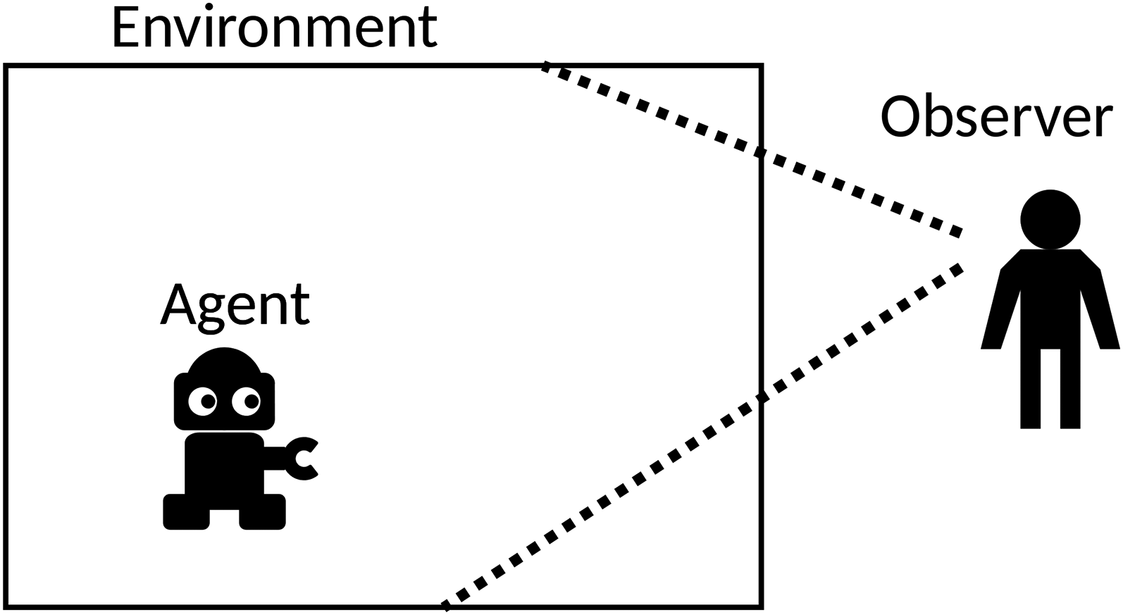
Agent in Its Environment and a Passive Observer.

Figure 2.

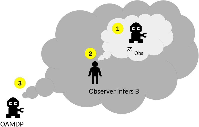
An Observer-Aware Markov Decision Process (OAMDP) Agent (3) Assumes that the Observer’s Expectation (2) Is that the Agent Behaves so as to Achieve Some Task (1).

Our objective in this paper is to propose a more satisfying approach to predictability by working not with complete trajectories, but with actions or states at each time step. This implies reasoning on dynamic variables, which requires introducing a variant of the OAMDP formalism. Moreover, we also consider not only discounted problems, but also stochastic shortest-path (i.e., goal-oriented) problems.

Section 2 provides background on MDPs and observer-aware MDPs. Our approach to action and state predictability, through dedicated reward functions, is described in Section 3, along with proof that well-defined problems are induced. Experiments are then presented in Section 4, where we generate and interpret policies on two types of grid-world problems, comparing with standard MDP solution policies, and then, in Section 5, where human observers are confronted with these policies on some of these problems.

2. Background

Notations: Sets will be denoted with calligraphic capital letters, for example, $\mathcal{X}$ , and random variables with normal capital letters, for example, $X$ . We will denote $\mathrm{\Delta }(\mathcal{X})$ the probability simplex over some finite set $\mathcal{X}$ , that is, the set of probability distributions over $X$ .

2.1. Markov Decision Processes (MDPs)

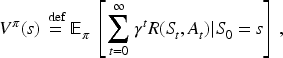
An MDP (Bellman, 1957) is specified through a tuple $⟨\mathcal{S},\mathcal{A},T,R,\gamma ,{\mathcal{S}}_{\mathcal{T}}⟩$ where:

$\mathcal{S}$ is a set of states;

$\mathcal{A}$ is a set of actions;

$T:\mathcal{S}\times \mathcal{A}\times \mathcal{S}\to [0;1]$ , the transition function, gives the probability $T(s,a,s^{\prime })$ that action $a$ performed in state $s$ will lead to state $s^{\prime }$ ;

$R:\mathcal{S}\times \mathcal{A}\times \mathcal{S}\to \mathbb{R}$ , the reward function, gives the immediate reward $R(s,a,s^{\prime })$ received upon transition $(s,a,s^{\prime })$ .

$\gamma \in [0,1]$ is a discount factor; and

${\mathcal{S}}_{\mathcal{T}}\subset \mathcal{S}$ is a set of terminal states: for all $s,a\in \mathcal{S}\times \mathcal{A}$ , $T(s,a,s)=1$ and $R(s,a,s)=0$ .

Then, a (stochastic) policy $\pi :\mathcal{S}\to \mathrm{\Delta }(\mathcal{A})$ maps states to distributions over actions, $\pi (a|s)$ denoting the probability to perform $a$ when in $s$ . When a policy is deterministic, $\pi (s)$ denotes the only possible action in $s$ . Assuming $\gamma <1$ , the value of a policy $\pi$ is the sum of discounted rewards on an infinite horizon:

$$V^{\pi }(s)\stackrel{\mathrm{def}}{=}{\mathbb{E}}_{\pi }[\sum _{t=0}^{\mathrm{\infty }}{\gamma }^{t}R(S_t,A_t)|S_0=s],$$

and an optimal policy ${\pi }^{*}$ is such that, for all $s$ , $V^{\pi *}(s)=\underset{\pi }{max}{V}^{\pi }(s)$ . The value iteration (VI) algorithm (Bellman, 1957) approximates $V^{*}$ , the value function common to all optimal policies, by iterating the following computation (where $k$ is the current iteration):

$$V_k(s)\leftarrow \underset{a}{max}\sum _{s^{\prime }}T(s,a,s^{\prime })\cdot (R(s,a,s^{\prime })+\gamma V_{k-1}(s^{\prime })).$$

Calculations stop when the Bellman residual is below a threshold:

$$\underset{\text{Bellman residual}}{\underbrace{\underset{s}{max}|V_k(s)-V_{k-1}(s)|}}\le \frac{1-\gamma }{\gamma }ϵ.$$

Then, an $ϵ$ -optimal policy is obtained by acting greedily with respect to the solution value function $V_k$ , that is, using

$${\pi }_k(s)\leftarrow {\arg \max }_a\sum _{s^{\prime }}T(s,a,s^{\prime })\cdot (R(s,a,s^{\prime })+\gamma V_k(s^{\prime })).$$

The same dynamic programming operator may still be contracting, thus apply, when $\gamma =1$ , in so-called shortest-path problems (SSPs; Bertsekas, 2005; Hansen & Zilberstein, 2001), that is, problems whose objective is to reach a terminal state (meaning that ${\mathcal{S}}_{\mathcal{T}}$ is not empty) at minimum expected cost (opposite of reward). SSPs are more general than MDPs because any MDP can be turned into an SSP with, at any time step, a $1-\gamma$ probability to transition to a terminal state (Bertsekas, 2005, Section 7.3). SSPs are more general than MDPs because any MDP can be turned into an SSP with, at any time step, a $1-\gamma$ probability to transition to a terminal state (Bertsekas, 2005, Section 7.3). Note: No stopping criterion provides guarantees about the solution quality in general SSPs (cf. Hansen, 2017). So, here, we simply stop the algorithm when the Bellman residual is below some threshold $\eta \ll ϵ$ and assume that $V$ is $ϵ$ -close to $V^{*}$ .

Let us call proper a policy $\pi$ that reaches ${\mathcal{S}}_{\mathcal{T}}$ with probability $1$ from any state. We will from now on focus on valid SSPs (and may omit the term “valid”), that is, SSPs verifying the following assumptions:

(A1) for any policy $\pi$ and any state $s$ , $\pi$ reaches ${\mathcal{S}}_{\mathcal{T}}$ with probability 1 from $s$ iff $V^{\pi }(s)>-\mathrm{\infty }$ ; and (A2) at least one proper policy $\pi$ exists (i.e. $\mathrm{\forall }s$ , $V^{\pi }(s)>-\mathrm{\infty }$ ).

In particular, the first assumption holds if, for all $(s,a,s^{\prime })\in (\mathcal{S}\setminus {\mathcal{S}}_{\mathcal{T}})\times \mathcal{A}\times (\mathcal{S}\setminus {\mathcal{S}}_{\mathcal{T}})$ , $R(s,a,s^{\prime })<0$ .

2.2. Observer-Aware MDPs (OAMDPs)

As introduced by Miura and Zilberstein (2021), an OAMDP models a situation wherein an agent attempts to maximize an observer’s information regarding some target random variable, called type, under some model of the observer’s evolving belief about this type. Formally, an OAMDP is described by aneight-tuple $⟨\mathcal{S},\mathcal{A},T,\gamma ,{\mathcal{S}}_{\mathcal{T}},\mathrm{\Theta },B,R⟩$ , where:

$⟨\mathcal{S},\mathcal{A},T,\gamma ,{\mathcal{S}}_{\mathcal{T}}⟩$ is a rewardless discounted MDP ( $\gamma <1$ );

$\mathrm{\Theta }$ is a finite set of types representing a characteristic of the agent such as possible goals, intentions, or capabilities;

$B:H^{*}\to \mathrm{\Delta }(\mathrm{\Theta })$ gives the assumed belief of the observer given a history ( $H=\mathcal{S}\times \mathcal{A}$ );

$R:\mathcal{S}\times \mathcal{A}\times \mathrm{\Delta }(\mathrm{\Theta })\to \mathbb{R}$ is the reward function; it allows formalizing the agent’s actual objective, for example, regarding legibility, explainability, or predictability.

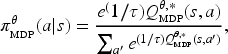
In most of the cases they consider, Miura and Zilberstein derive $B$ by relying on Baker et al.’s (2009) “BST” ¹ Bayesian belief update rule, that is, considering that, again from the agent’s viewpoint, the observer models the agent’s behavior for a given type through an MDP by

using a corresponding reward function $R_{\mathcal{m}\mathcal{d}\mathcal{p}}^{\theta }$ , that is, assuming that, when of type $\theta$ , the agent optimizes $R_{\mathcal{m}\mathcal{d}\mathcal{p}}^{\theta }$ ;

solving the discounted MDP $⟨\mathcal{S},\mathcal{A},T,R_{\mathcal{m}\mathcal{d}\mathcal{p}}^{\theta },\gamma ,{\mathcal{S}}_{\mathcal{T}}⟩$ (where all components but $R_{\mathcal{m}\mathcal{d}\mathcal{p}}^{\theta }$ come from the OAMDP definition) to obtain $V_{\mathcal{m}\mathcal{d}\mathcal{p}}^{\theta ,*}$ ;

building a stochastic “softmax” policy—that is, the policy that the agent is supposed to follow if of type $\theta$ —such that, $\mathrm{\forall }(s,a)$ ,

$$\begin{array}{rl}{\pi }_{\mathcal{m}\mathcal{d}\mathcal{p}}^{\theta }(a|s)& =\frac{e^{(}1/\tau )Q_{\mathcal{m}\mathcal{d}\mathcal{p}}^{\theta ,*}(s,a)}{\sum _{a^{\prime }}{e}^{(1/\tau )Q_{\mathcal{m}\mathcal{d}\mathcal{p}}^{\theta ,*}(s,a^{\prime })}},\end{array}$$

where

$$\begin{array}{rl}{Q}_{\mathcal{m}\mathcal{d}\mathcal{p}}^{\theta ,*}(s,a)& =\sum _{s^{\prime }}T(s,a,s^{\prime })\cdot (r(s,a,s^{\prime })+\gamma V_{\mathcal{m}\mathcal{d}\mathcal{p}}^{\theta ,*}(s^{\prime })),\end{array}$$

and temperature $\tau >0$ allows tuning the policy’s optimality (thus the agent’s assumed rationality for the observer).

With ${\pi }_{\mathcal{m}\mathcal{d}\mathcal{p}}\equiv ({\pi }_{\mathcal{m}\mathcal{d}\mathcal{p}}^{\theta }{)}_{\theta \in \mathrm{\Theta }}$ in hand, the observer’s belief function about the type can then be obtained through Bayesian inference.

Miura and Zilberstein (2021) use the OAMDP framework to formalize various observer-aware problems from the literature, including legibility, explainability, and predictability. For predictability, which we now focus on, they mention two approaches. The first one builds on Dragan et al.’s (2013) idea to “model the predictability of a trajectory as simply proportional to the value (negative cost) of a trajectory,” which, in the OAMDP setting, translates into (1) having a single type ${\theta }^0$ , and (2) optimizing the underlying reward function $R_{\mathcal{m}\mathcal{d}\mathcal{p}}^{{\theta }^0}$ , that is, acting greedily wrt $Q_{\mathcal{m}\mathcal{d}\mathcal{p}}^{{\theta }^0,*}$ (rather than following ${\pi }_{\mathcal{m}\mathcal{d}\mathcal{p}}^{{\theta }^0}$ ). The second approach builds on Fisac et al.’s (2020) $t$ -predictability, which maximizes $Pr(a_{t+1},\dots ,a_T|a_1,\dots ,a_t)$ in deterministic settings, by using a type for each possible trajectory—that is, exponentially many types—over a finite temporal horizon.

To wrap up, in the OAMDP framework, typically using the BST update, the agent (i) assumes that the observer models the agent, when of type $\theta$ , as following a softmax policy ${\pi }_{\mathcal{m}\mathcal{d}\mathcal{p}}^{\theta }$ that near-optimally cumulates rewards $R_{\mathcal{m}\mathcal{d}\mathcal{p}}^{\theta }$ , and accordingly updates its belief about the agent’s type in a Bayesian manner (which defines $B$ ); (ii) then computes an actual solution policy maximizing the cumulative rewards $R$ , accounting for the evolution of both the system state and the observer’s belief.

In the following, we propose an alternative approach to predictability and discuss its properties.

3. Contribution

As a preliminary contribution, while Miura and Zilberstein consider only discounted OAMDPs, we introduce observer-aware SSPs (OASSPs; thus, using $\gamma =1$ ). This mainly raises the question: Under which conditions do proper policies exist in the induced SSP? We will discuss this issue in the context of predictability.

3.1. Predictable Observer-Aware MDPs (pOAMDPs)

Both approaches to predictability mentioned by Miura and Zilberstein are inspired by work in deterministic settings, reasoning on trajectories. Because both the softmax policy ${\pi }_{\mathcal{m}\mathcal{d}\mathcal{p}}$ and the dynamics of the system can be stochastic, we instead propose to try predicting either actions or states, both alternatives (action and state predictability) possibly leading to different solutions. Yet, OAMDP types $\theta$ are static variables (as types in Bayesian games; Fudenberg & Tirole, 1991; Harsanyi, 1967), while actions and states are dynamic. This leads us to introduce pOAMDPs, where we instead talk of a (dynamic) target variable, also noted ${\theta }_t$ , which is now a function of the current transition: ${\theta }_t=\varphi (s_t,a_t,s_{t+1})$ . This (1) does not allow encoding problems where the target variable is static and hidden (i.e., is a type), for example, legibility or explicability, but (2) still allows (a) defining and solving the observer’s MDP (because the type does not influence the system dynamics), and (b) using the BST belief update (because of the Markovian nature of the target variables).

The following sections describe, respectively, both action and state predictability: (1) how to derive $B$ and solve the pOAMDP given a reward function $R$ , and (2) the reward functions proposed to formalize predictability, along with properties of the resulting decision problems.

3.2. Belief Function and Properties of pOAMDPs

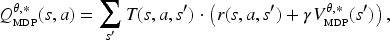
For action predictability, $\mathrm{\Theta }=\mathcal{A}$ , $\varphi (s,a,s^{\prime })=a$ , and $B$ is

$$\begin{array}{rl}B:& \begin{array}{ccc}{H}^{*}& \to & \mathrm{\Delta }(\mathcal{A}),\\ (s_0,a_0,\dots ,s_t)& \mapsto & {\pi }_{\mathcal{m}\mathcal{d}\mathcal{p}}(A_t|s_t).\end{array}\end{array}$$

For state predictability, $\mathrm{\Theta }=\mathcal{S}$ , $\varphi (s,a,s^{\prime })=s^{\prime }$ , and $B$ is

$$\begin{array}{rl}B:& \begin{array}{ccc}{H}^{*}& \to & \mathrm{\Delta }(\mathcal{S}),\\ (s_0,a_0,\dots ,s_t)& \mapsto & \sum _{a^{\prime }}{\pi }_{\mathcal{m}\mathcal{d}\mathcal{p}}(a^{\prime }|s_t)\cdot T(s_t,a^{\prime },S_{t+1}).\end{array}\end{array}$$

In both cases, since $B$ depends only on the current state, $s_t$ , we can denote the belief about target variable $\theta$ under $s_t$ as $B(s_t)=b_{s_t}(\theta )$ and redefine the pOAMDP reward function (not the observer’s one) as $R^{\prime }(s_t,a_t)\stackrel{\mathrm{def}}{=}R(s_t,a_t,b_{s_t}(\theta ))$ instead of $R(s_t,a_t,B(s_0,a_0,\dots ,s_t))$ .

The agent’s sequential decision-making problem can then be expressed as an MDP $⟨\mathcal{S},\mathcal{A},T,R^{\prime },\gamma ,{\mathcal{S}}_{\mathcal{T}}⟩$ solvable with an algorithm such as VI. The solving complexity is thus the complexity of solving both the observer MDP and the MDP induced by the pOAMDP. In contrast, in the case of OAMDPs (Miura & Zilberstein, 2021), one generally cannot obtain such an MDP, and solving the OAMDP requires specific algorithms in which the action choice is linked to the whole state-action history (so that the tree of possible futures that needs to be accounted for grows exponentially with the size of the history).

3.3. pOAMDP Reward Function

Reward Definition

When in state $s$ , to predict the next target variable’s value (action or state) as well as possible, the observer should pick one of the most likely values according to her model of the agent’s behavior. This means picking an action in ${\arg \max }_{a\in \mathcal{A}}{b}_s(a)$ (or a state in ${\arg \max }_{s^{\prime }\in \mathcal{S}}{b}_s(s^{\prime })$ ). We will assume that the observer samples her prediction uniformly from this set, and thus define $\text{pred}(\theta |s)\stackrel{\mathrm{def}}{=}1/|{\arg \max }_{\theta \in \mathrm{\Theta }}{b}_s(\theta )|$ if $\theta \in {\arg \max }_{\theta \in \mathrm{\Theta }}{b}_s(\theta )$ , and $0$ otherwise. Note: From now on, we focus on action predictability, only highlighting some points for state predictability.

Then, considering an SSP (thus with $\gamma =1$ ), we would like to minimize the expected number of prediction errors made by the observer along a trajectory. For a single transition $(s,a,s^{\prime })$ , assuming the above model of observer prediction, the probability of a bad action prediction is $1-\text{pred}(a|s)$ . Because we are in a maximization rather than a minimization setting, and generalizing the formula to both action and state predictabilities, this leads to defining the reward function as:

$$R_{\text{pred}}^{\mathrm{\Theta }}(s,a,s^{\prime })\stackrel{def}{=}\text{pred}(\varphi (s,a,s^{\prime })|s)-1.$$

Then, in any state $s$ , $-V^{*}(s)$ gives the expected number of future prediction errors.

Valid SSPs?

An important question is whether this reward function induces a valid SSP, that is, whether assumptions (A1) and (A2) are satisfied.

Proposition 1

Let us assume that (i) $\gamma =1$ , (ii) the MDP considered by the observer is a valid SSP, and (iii) $R_{\text{pred}}^{\mathcal{A}}$ is the pOAMDP reward function. Then the pOAMDP is a well-defined problem as its induced SSP satisfies assumptions (A1) and (A2).

Proof.

(A1) Let $\pi$ be any policy and $s$ be any state and then proceed in two steps:

Assume $\pi$ reaches ${\mathcal{S}}_{\mathcal{T}}$ with probability $1$ from $s$ . Then, trivially, $V^{\pi }(s)>-\mathrm{\infty }$ .

Assume $\pi$ does not reach ${\mathcal{S}}_{\mathcal{T}}$ with probability $1$ from $s$ . Then $s$ is in some subset ${\mathcal{S}}^{\prime }\subseteq (\mathcal{S}\setminus {\mathcal{S}}_{\mathcal{T}})$ that is connex under $\pi$ , that is, once reached, all states are visited infinitely often. Let ${\pi }_{\mathcal{m}\mathcal{d}\mathcal{p}}^{*}$ be an optimal policy of the observer SSP. Because the observer SSP is valid, thus eventually reaches a terminal state, there exists a state $s^{\prime }\in {\mathcal{S}}^{\prime }$ in which ${\pi }_{\mathcal{m}\mathcal{d}\mathcal{p}}^{*}(s^{\prime })$ can transition outside of ${\mathcal{S}}^{\prime }$ with nonzero probability, meaning that ${\pi }_{\mathcal{m}\mathcal{d}\mathcal{p}}^{*}(s^{\prime })\ne \pi (s^{\prime })$ . As a consequence, $\text{pred}(\pi (s^{\prime })|s^{\prime })<1$ and $R_{\text{pred}}^{\mathcal{A}}(s^{\prime },\pi (s^{\prime }),s^{″})<0$ for any $s^{″}$ . $s^{\prime }$ being visited infinitely often under $\pi$ , we have in particular that $V^{\pi }(s)=-\mathrm{\infty }$ .

This proves that (A1) holds.

(A2) Let us point out that whether a policy is proper or not depends on the reachability of terminal states, not on the reward function. Since the observer SSP satisfies assumption (A2) and only differs from the predictable observer-aware shortest-path problem (pOASSP) in its rewards function, the induced SSP also satisfies assumption (A2).

This result does not hold for state predictability.

Proposition 2

Let us assume that (i) $\gamma =1$ , (ii) the MDP considered by the observer is a valid SSP, and (iii) $R_{\text{pred}}^{\mathcal{S}}$ is the pOAMDP reward function. Then the pOAMDP may be an ill-defined problem as its induced SSP satisfies assumption (A2), but may not satisfy assumption (A1).

Proof.

The proof that assumption (A2) holds is the same as for action predictability.

To prove that assumption (A1) may not hold, let us consider an OAMDP with:

$\mathcal{S}=\{s_0,s_G\}$ , with $s_0$ initial and $s_G$ terminal;

$\mathcal{A}=\{a_1,a_2\}$ ;

the transition function described in Figure 3;

$r_{\mathcal{m}\mathcal{d}\mathcal{p}}(s_0,a,s^{\prime })=1$ for all $a$ and $s^{\prime }$ ; and

the state-predictability reward function.

Figure 3.

Transition Function of an Ill-Defined Predictable Observer-Aware Shortest-Path Problem (pOASSP) for State Predictability, with Transition Probabilities as Edge Labels.

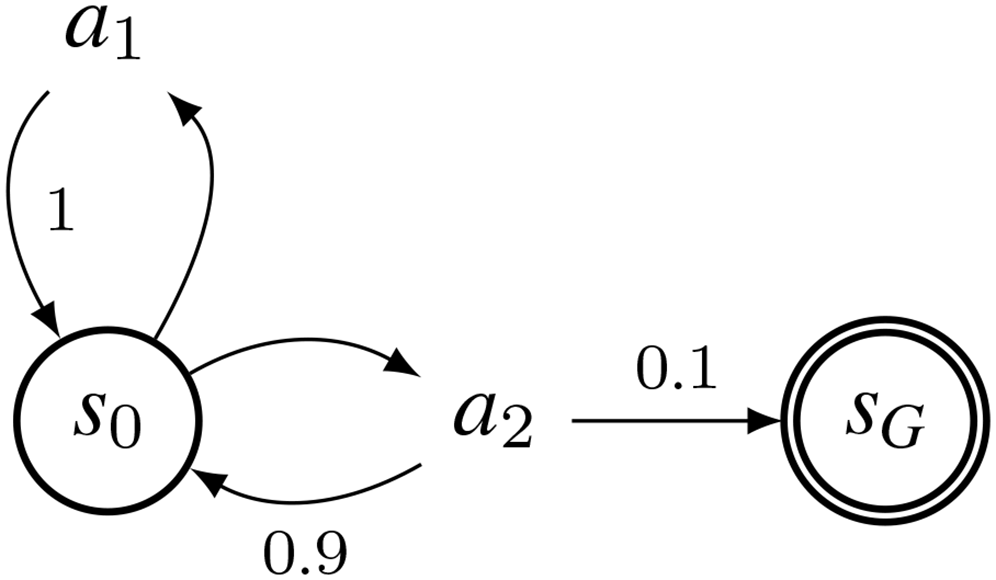
In this setting, due to the transition function, when applying ${\pi }_{\mathcal{m}\mathcal{d}\mathcal{p}}$ in $s_0$ , the most probable next state is $s_0$ , meaning that the observer should bet on $s_0$ . As a consequence, we can evaluate the policies ${\pi }_{a_1}$ and ${\pi }_{a_2}$ that, respectively, always pick $a_1$ and $a_2$ when in $s_0$ :

$$\begin{array}{rl}{V}^{{\pi }_{a_1}}(s_0)& =T(s_0,a_1,s_0)\cdot (R_{\text{pred}}^{\mathcal{S}}(s_0,a_1,s_0)+V^{{\pi }_{a_1}}(s_0))\end{array}$$

(1)

$$\begin{array}{rl}& =1\cdot (0+V^{{\pi }_{a_1}}(s_0))\end{array}$$

(2)

$$\begin{array}{rl}& =0{,}^{\text{[One could argue that the value is undefined.]}}\end{array}$$

(3)

and

$$\begin{array}{rl}{V}^{{\pi }_{a_2}}(s_0)& =T(s_0,a_2,s_0)\cdot (R_{\text{pred}}^{\mathcal{S}}(s_0,a_2,s_0)+V^{{\pi }_{a_2}}(s_0))\end{array}$$

(4)

$$\begin{array}{rl}& +T(s_0,a_2,s_G)\cdot (R_{\text{pred}}^{\mathcal{S}}(s_0,a_2,s_G)+V^{{\pi }_{a_2}}(s_G))\end{array}$$

(5)

$$\begin{array}{rl}& =0.9\cdot (0+V^{{\pi }_{a_2}}(s_0))+0.1\cdot (-1+0)\end{array}$$

(6)

$$\begin{array}{rl}& =0.9\cdot V^{{\pi }_{a_2}}(s_0)-0.1\end{array}$$

(7)

$$\begin{array}{rl}& =-1.\end{array}$$

(8)

${\pi }_{a_1}$ is thus the only optimal policy for state predictability, although it never reaches the terminal state, which breaks assumption (A1).

This negative result does not prevent from using $R_{\text{pred}}^{\mathcal{S}}$ in OASSPs, in particular:

if linearly combined with another reward function that necessarily induces a valid SSP, for example, $R_{\text{pred}}^{\mathcal{A}}$ or a nonpositive reward function (such as $R(s,a,s^{\prime })=-1$ for any $(s,a,s^{\prime })$ ); and

in case of deterministic dynamics; indeed, if a policy $\pi$ induces an absorbing subset of states ${\mathcal{S}}^{\prime }\subseteq \mathcal{S}\setminus {\mathcal{S}}_{\mathcal{T}}$ , then $T(s,\pi (s))\ne T(s,{\pi }_{\mathcal{m}\mathcal{d}\mathcal{p}}(s))$ for some $s\in {\mathcal{S}}^{\prime }$ , so that $R_{\text{pred}}^{\mathcal{S}}(s,\pi (s),T(s,\pi (s)))<0$ , meaning that $\pi$ has a negative infinite value at least in $s$ (so that assumption (A1) holds).

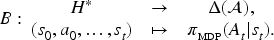
In the case of (discounted) MDPs, we will rely on the same reward definition. The interpretation of $-V^{*}(s)$ is similar if one sees the problem as an equivalent SSP with a $1-\gamma$ termination probability at each time step.

This section introduced the pOAMDP formalism, including two reward functions—based on the idea of rewarding successful guesses—to express action- and state-predictability problems. It also showed that OAMDPs with BST updates are addressed by solving two MDPs consecutively, and demonstrated that, while action predictability induces valid SSPs, this may not be the case for state predictability.

The next two sections study this approach to action and state predictability on simple examples: (1) in silico, observing and analyzing the policies obtained through our approach, and compared with simple MDP policies; and (2) in vivo, that is, confronting actual human observers with several policies.

4. Generating and Interpreting Policies

These first experiments aim at illustrating and better understanding the policies induced by the proposed reward function, and in particular at determining whether they can be considered as predictable. The code is available under an open license here: https://gitlab.inria.fr/po-OAMDP/predictable-OAMDP_ejai25.

4.1. Protocol

To describe the two types of pOAMDPs considered in our experiments, let us just detail the corresponding MDPs, both set in four-connected grid worlds, that the observer will take into account:

an SSP, named maze, in which a robot wants to reach a terminal goal state; and

a discounted MDP (with no terminal state), named firefighter, in which a robot uses water sources to extinguish fires.

To facilitate the analysis, the dynamics of both problems is mostly deterministic.

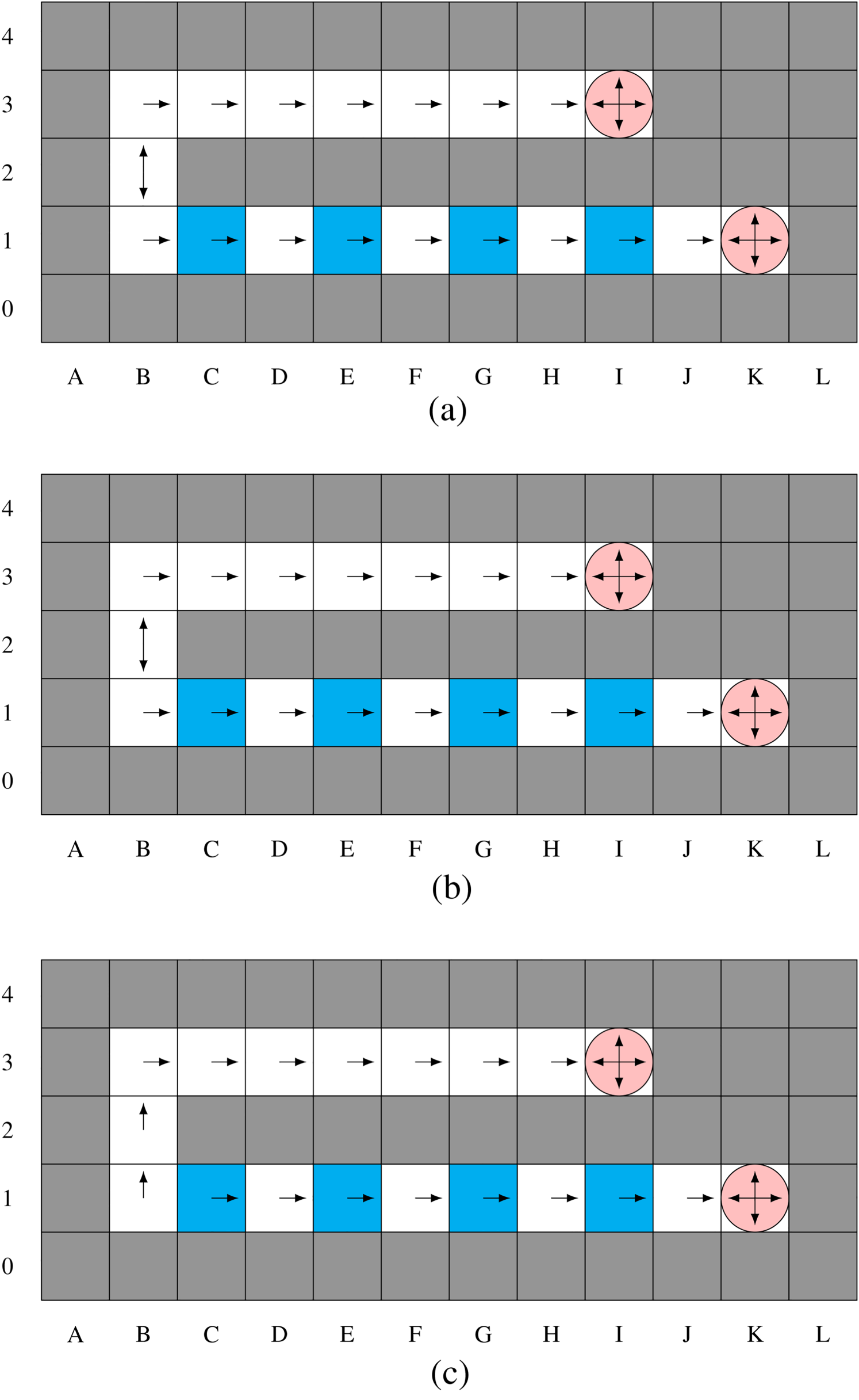
Maze problem

A maze (cf. Figure 4) contains walls (in dark gray), normal cells (in white), slippery cells (in cyan), and terminal cells (pink disks). The starting cell is marked by a circle. More formally, in this SSP:

each state $s$ in $\mathcal{S}$ indicates the $(x,y)$ coordinates of the robot in a normal, slippery, or terminal cell;

${\mathcal{S}}_{\mathcal{T}}$ is a nonempty (but also possibly nonsingleton) subset of $\mathcal{S}$ ;

$\mathcal{A}=\{\mathrm{up},down,left,right\}$ ;

$T(s,a,s^{\prime })$ encodes the robot’s moves: a robot in a normal cell moves in the direction indicated by its action if no wall prevents it; in a slippery cell, the robot has a probability $p$ ( $0.5$ in our experiments) of making a two-cell rather than one-cell move (if possible); in a terminal cell, the robot does not move;

$R_{\mathcal{m}\mathcal{d}\mathcal{p}}$ , the reward function, returns

$*$

a default penalty of $-0.04$ for each move,

$*$

$-1$ when the robot hits a wall,

$*$

$+1$ upon reaching a terminal state $s_f$ , and

$*$

$0$ when the robot stays in the terminal state.

This SSP trivially satisfies assumptions (A1) and (A2).

Figure 4.

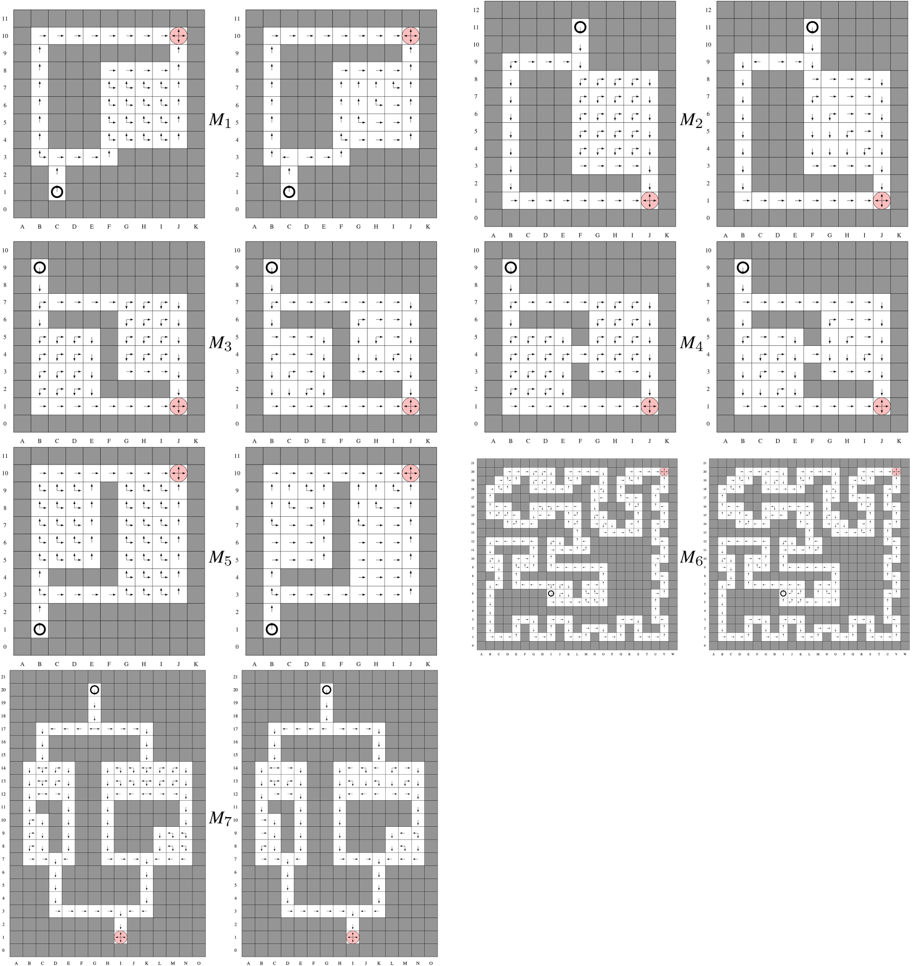
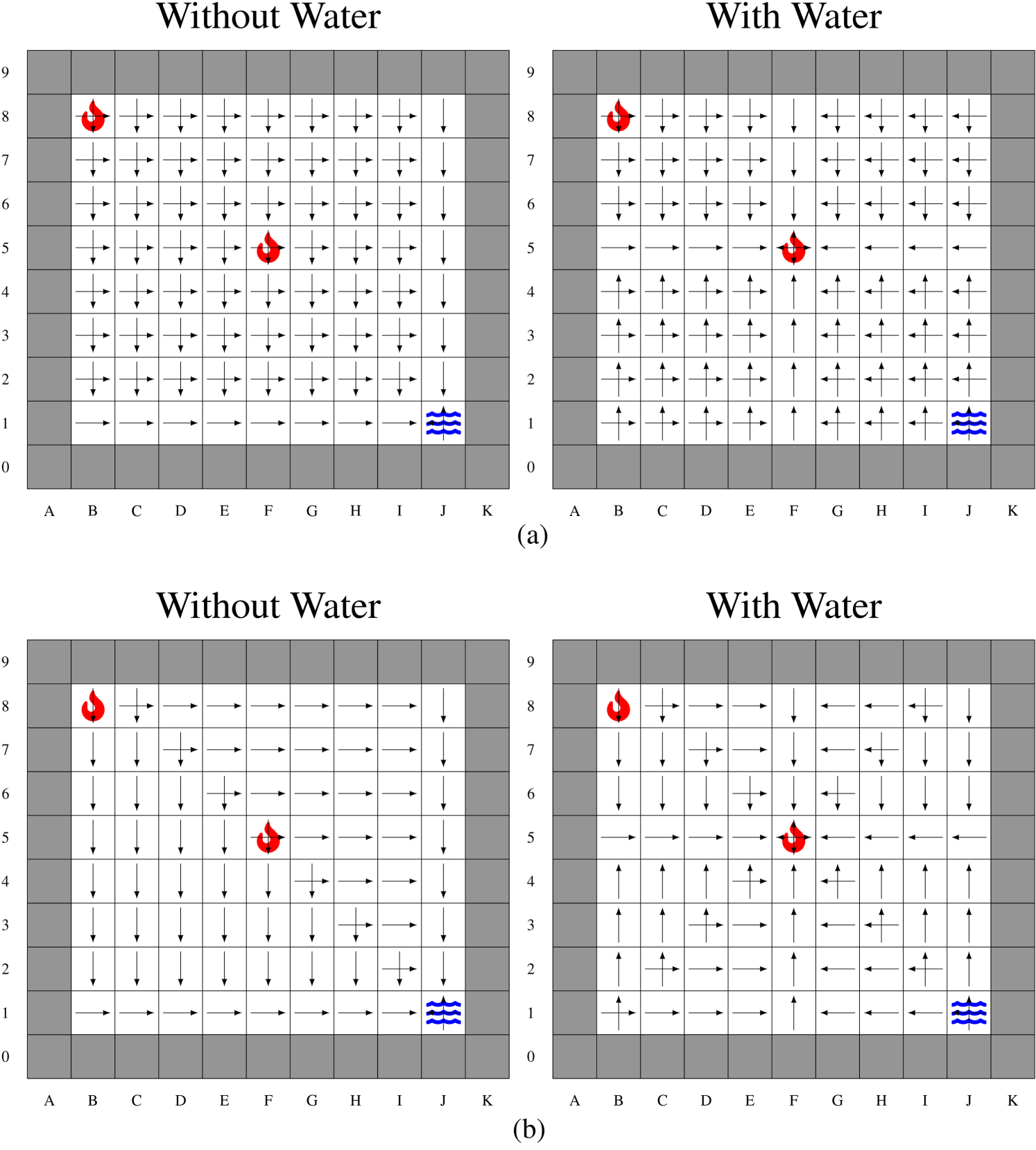
Action Predictability Results Showing, for Mazes $M_1$ – $M_7$ , the Stochastic Policy ${\pi }_{\mathcal{m}\mathcal{d}\mathcal{p}\mathcal{-}\mathcal{s}}$ (Left) (which “covers” all Deterministic Policies ${\pi }_{\mathcal{m}\mathcal{d}\mathcal{p}\mathcal{-}\mathcal{b}}$ ) and the Observer-Aware Markov decision Process (OAMDP) Policy ${\pi }_{\text{pred}}^{\mathcal{A}}$ (Right). All Policies have been Computed Using $\gamma =1$ .

Firefighter Problem

Similar grids are used for the firefighter problem, but with terminal cells replaced by fires and water sources (cf. Figure 6). The robot now has a water tank, which is emptied upon reaching a (never extinguished) fire, and filled upon reaching a (never emptied) water source. More formally, in this $\gamma =0.99$ -discounted MDP:

each state $s$ in $\mathcal{S}$ is represented by a triplet $(x,y,w)$ with $(x,y)$ the robot’s coordinates and $w$ a boolean encoding whether its water tank is full;

$\mathcal{A}=\{\mathrm{up},down,left,right\}$ ;

$T(s,a,s^{\prime })$ is similar to the maze problem, except that $w$ becomes false upon reaching a fire and true upon reaching a water source;

$R_{\mathcal{m}\mathcal{d}\mathcal{p}}$ , the reward function, returns

• $*$

a default penalty of $-0.04$ for each move,

$*$

$-1$ when the robot hits a wall, and

$*$

$+1$ when the robot reaches a fire while carrying water ( $w=$ true).

Optimal MDP policies consist of endlessly going back and forth between a water source and a fire.

Baseline Policies

The pOAMDP solution policy, denoted ${\pi }_{\text{pred}}^{\mathrm{\Theta }}$ , will be compared with near-optimal solutions of the observer MDP obtained as follows. We solve the observer MDP until convergence to an $ϵ$ -optimal value function. Then, in each state $s$ , let $\psi (s)\stackrel{\mathrm{def}}{=}\{a\in \mathcal{A}|Q^{*}(s,a)\ge V^{*}(s,a)-2ϵ\}$ . This set necessarily contains all optimal actions. With this, we can first define ${\pi }_{\mathcal{m}\mathcal{d}\mathcal{p}\mathcal{-}\mathcal{s}}$ , a stochastic policy that, in each state $s$ , samples actions uniformly from $\psi (s)$ .

In practice, algorithms will often be biased, having a preference order over actions. We thus also consider the policies that, in each state $s$ , deterministically pick the preferred action given a predefined order. These biased (and deterministic) policies are denoted ${\pi }_{\mathcal{m}\mathcal{d}\mathcal{p}\mathcal{-}\mathcal{b}}$ , not distinguishing them from each other.

pOAMDP Model

For both types of problems and each grid environment, a pOAMDP is derived using the previously proposed reward function for predictability $R_{\text{pred}}^{\mathrm{\Theta }}$ . The baseline policy ${\pi }_{\mathcal{m}\mathcal{d}\mathcal{p}\mathcal{-}\mathcal{s}}$ described above serves to identify the observer’s possible predictions. Since each pOAMDP can be considered as an MDP, pOAMDPs are solved by using again the VI algorithm with an appropriate discount factor (details in the next section), resulting in the $R_{\text{pred}}^{\mathrm{\Theta }}$ policy. Note that our approach does not make use of the softmax policy, thus making its temperature parameter $\tau$ irrelevant.

4.2. Results

The figures present both stochastic MDP policies ${\pi }_{\mathcal{m}\mathcal{d}\mathcal{p}\mathcal{-}\mathcal{s}}$ (which also “cover” all deterministic policies ${\pi }_{\mathcal{m}\mathcal{d}\mathcal{p}\mathcal{-}\mathcal{b}}$ ), and pOAMDP policies ${\pi }_{\text{pred}}^{\mathrm{\Theta }}$ , the arrows indicating all $ϵ$ -optimal actions.

4.2.1. Maze Problem

Grids Used

The mazes mainly consist of corridors and (empty) rooms.

For action predictability, we expect the pOAMDP policies to prefer corridors over rooms (which allow for more possible optimal actions). Figure 4 shows mazes $M_1$ – $M_7$ , which have been used for action predictability (including experiments with humans discussed in Section 5). They all consist of a number of corridors and rooms, have a starting state $s_0$ (marked by a circle), and an overall increase in complexity from $M_1$ to $M_7$ . The maze $M_8$ in Figure 5 consists of two corridors that lead to a terminal state. One of these corridors contains slippery cells, but the average traversal time is the same for both. This maze’s goal is to observe differences between $R_{\text{pred}}^{\mathcal{A}}$ and $R_{\text{pred}}^{\mathcal{S}}$ .

Figure 5.

Results for Maze $M_8$ . (a) Stochastic Policy ${\pi }_{\mathcal{m}\mathcal{d}\mathcal{p}\mathcal{-}\mathcal{s}}$ ( $\gamma =1$ ); (b) Predictable Observer-Aware Markov Decision Process (pOAMDP) Policy ${\pi }_{\text{pred}}^{\mathcal{A}}$ ( $\gamma =1$ ); and (c) pOAMDP Policy ${\pi }_{\text{pred}}^{\mathcal{S}}$ ( $\gamma =1$ ).

Figure 6.

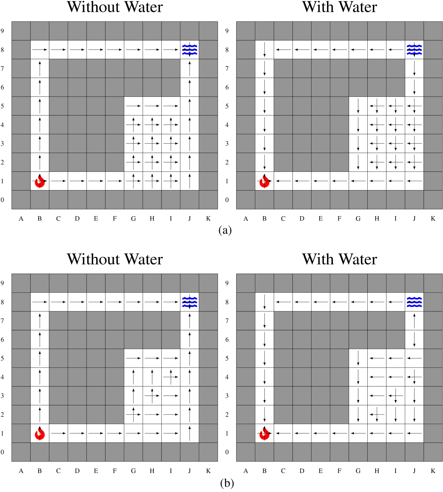
Results for Firefighter Problem F1. (a) Stochastic Policy ${\pi }_{\mathcal{m}\mathcal{d}\mathcal{p}\mathcal{-}\mathcal{s}}$ ( $\gamma =0.99$ ) and (b) pOAMDP Policy ${\pi }_{\text{pred}}^{\mathcal{A}}$ ( $\gamma =0.99$ ).

Each SSP is solved with $\gamma =1$ and $ϵ=0.001$ . As expected, when crossing a room of size $n\times m$ from one corner to the opposite corner, ${\pi }_{\mathcal{m}\mathcal{d}\mathcal{p}\mathcal{-}\mathcal{s}}$ randomly picks one of the $(\genfrac{}{}{0ex}{}{n+m}{n})$ optimal paths, while the only two possible ${\pi }_{\mathcal{m}\mathcal{d}\mathcal{p}\mathcal{-}\mathcal{b}}$ policies follow the walls (clockwise or counterclockwise).

Note: In the following, we mainly focus on action predictability because, here, solution policies turn out to be identical to state predictability. This is favored in deterministic environments, where predicting the next state is often equivalent to predicting the next action.

Analysis of ${\pi }_{\text{pred}}^{\mathcal{A}}$ and ${\pi }_{\text{pred}}^{\mathcal{S}}$

We observe several interesting behaviors with $R_{\text{pred}}^{\mathcal{A}}(s,a,s^{\prime })$ :

The pOAMDP robot (/agent) will plan a longer path through a narrow corridor, where its next action will be easy to predict, rather than a shorter path going through one or multiple rooms as illustrated on $M_1$ and $M_6$ .

In rooms, ${\pi }_{\mathcal{m}\mathcal{d}\mathcal{p}\mathcal{-}\mathcal{s}}$ has two optimal actions except along the two walls near the exit, with a single optimal action. The pOAMDP robot behaves thus more predictably by going toward the closest of these two exit walls and following it, as visible in $M_1$ – $M_7$ .

In $M_3$ , the pOAMDP robot can choose between (i) a corridor leading to a room and (ii) a room leading to a corridor. When $\gamma =1$ , the pOAMDP robot has no preference. When $\gamma <1$ (policy not shown here), the pOAMDP robot prefers to go through a corridor first because the discount puts more importance on early rewards (see cell $(B,7)$ ).

In $M_4$ , adding a door compared to $M_3$ makes for more uncertainty in the left room, so that the robot prefers going toward the right room.

In Figure 5, cell $(B,2)$ , ${\pi }_{\text{pred}}^{\mathcal{A}}$ has no preference between going up and down as, in both cases, there is no ambiguity about optimal actions afterward.

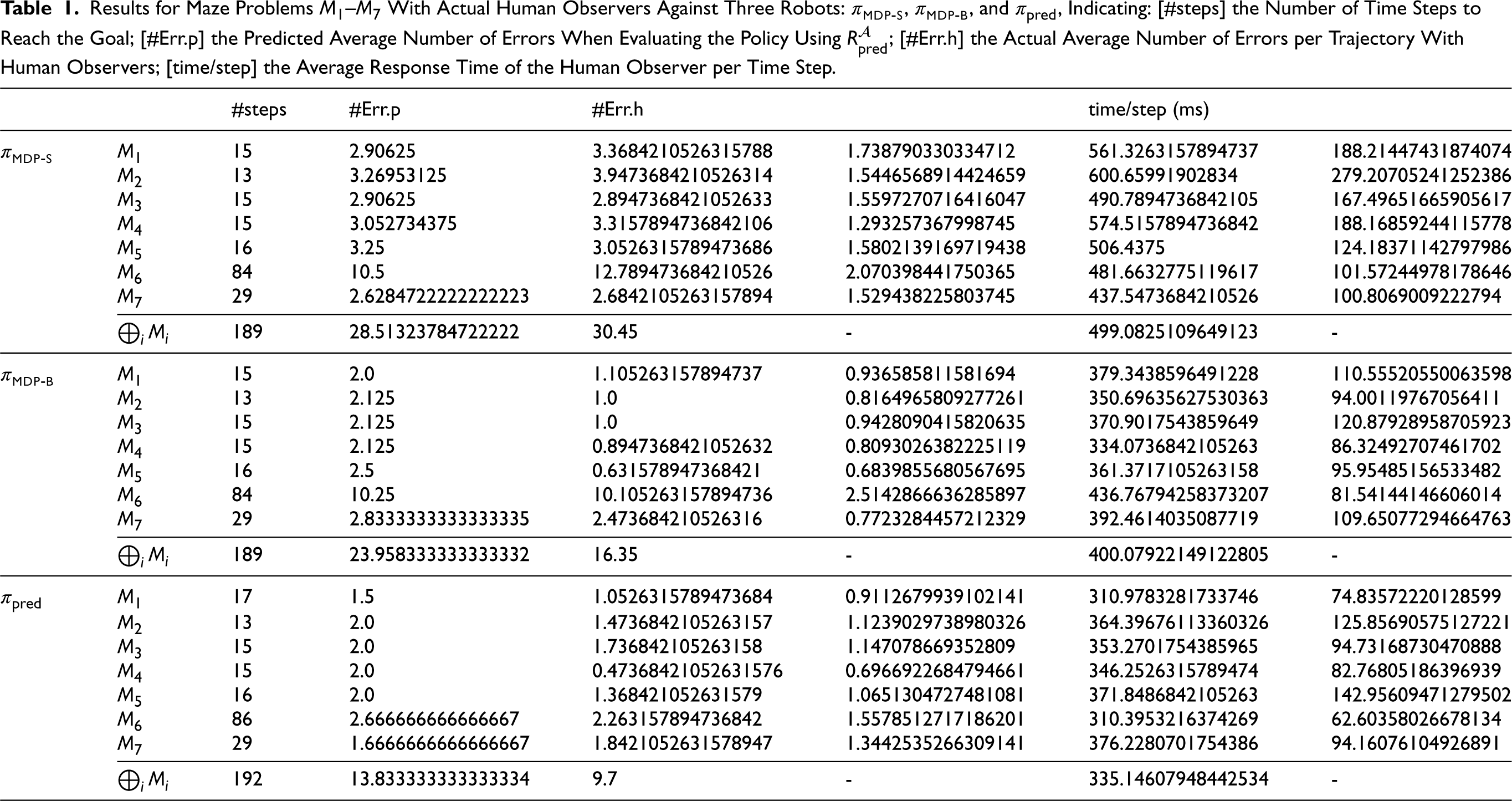
Quantitative results in the second column of Table 1 (#Err.p) are obtained by computing the value of each policy wrt $R_{\text{pred}}^{\mathcal{A}}$ and displaying $-V_{R_{\text{pred}}^{\mathcal{A}}}^{\pi }(s_0)$ . They show that ${\pi }_{\mathcal{m}\mathcal{d}\mathcal{p}\mathcal{-}\mathcal{s}}$ ’s expected number of errors per trajectory is worse than for the two other robot policies, in particular when large rooms exist. Also, ${\pi }_{\text{pred}}^{\mathcal{A}}$ has significantly better results than the two other policies on problems $M_6$ & $M_7$ , which have multiple rooms and are more complex.

Table 1.

Results for Maze Problems $M_1$ – $M_7$ With Actual Human Observers Against Three Robots: ${\pi }_{\mathcal{m}\mathcal{d}\mathcal{p}\mathcal{-}\mathcal{s}}$ , ${\pi }_{\mathcal{m}\mathcal{d}\mathcal{p}\mathcal{-}\mathcal{b}}$ , and ${\pi }_{\text{pred}}$ , Indicating: [#steps] the Number of Time Steps to Reach the Goal; [#Err.p] the Predicted Average Number of Errors When Evaluating the Policy Using $R_{\text{pred}}^{\mathcal{A}}$ ; [#Err.h] the Actual Average Number of Errors per Trajectory With Human Observers; [time/step] the Average Response Time of the Human Observer per Time Step.

		#steps	#Err.p	#Err.h		time/step (ms)
${\pi }_{\mathcal{m}\mathcal{d}\mathcal{p}\mathcal{-}\mathcal{s}}$	$M_1$	15	2.90625	3.3684210526315788	1.738790330334712	561.3263157894737	188.21447431874074
	$M_2$	13	3.26953125	3.9473684210526314	1.5446568914424659	600.65991902834	279.20705241252386
	$M_3$	15	2.90625	2.8947368421052633	1.5597270716416047	490.7894736842105	167.49651665905617
	$M_4$	15	3.052734375	3.3157894736842106	1.293257367998745	574.5157894736842	188.16859244115778
	$M_5$	16	3.25	3.0526315789473686	1.5802139169719438	506.4375	124.18371142797986
	$M_6$	84	10.5	12.789473684210526	2.070398441750365	481.6632775119617	101.57244978178646
	$M_7$	29	2.6284722222222223	2.6842105263157894	1.529438225803745	437.5473684210526	100.8069009222794
	$\underset{i}{⨁}{M}_i$	189	28.51323784722222	30.45	-	499.0825109649123	-
${\pi }_{\mathcal{m}\mathcal{d}\mathcal{p}\mathcal{-}\mathcal{b}}$	$M_1$	15	2.0	1.105263157894737	0.936585811581694	379.3438596491228	110.55520550063598
	$M_2$	13	2.125	1.0	0.8164965809277261	350.69635627530363	94.00119767056411
	$M_3$	15	2.125	1.0	0.9428090415820635	370.9017543859649	120.87928958705923
	$M_4$	15	2.125	0.8947368421052632	0.8093026382225119	334.0736842105263	86.32492707461702
	$M_5$	16	2.5	0.631578947368421	0.6839855680567695	361.3717105263158	95.95485156533482
	$M_6$	84	10.25	10.105263157894736	2.5142866636285897	436.76794258373207	81.54144146606014
	$M_7$	29	2.8333333333333335	2.473684210526316	0.7723284457212329	392.4614035087719	109.65077294664763
	$\underset{i}{⨁}{M}_i$	189	23.958333333333332	16.35	-	400.07922149122805	-
${\pi }_{\text{pred}}$	$M_1$	17	1.5	1.0526315789473684	0.9112679939102141	310.9783281733746	74.83572220128599
	$M_2$	13	2.0	1.4736842105263157	1.1239029738980326	364.39676113360326	125.85690575127221
	$M_3$	15	2.0	1.736842105263158	1.147078669352809	353.2701754385965	94.73168730470888
	$M_4$	15	2.0	0.47368421052631576	0.6966922684794661	346.2526315789474	82.76805186396939
	$M_5$	16	2.0	1.368421052631579	1.0651304727481081	371.8486842105263	142.95609471279502
	$M_6$	86	2.666666666666667	2.263157894736842	1.5578512717186201	310.3953216374269	62.60358026678134
	$M_7$	29	1.6666666666666667	1.8421052631578947	1.3442535266309141	376.2280701754386	94.16076104926891
	$\underset{i}{⨁}{M}_i$	192	13.833333333333334	9.7	-	335.14607948442534	-

In most of these problems, ${\pi }_{\text{pred}}^{\mathcal{A}}$ and ${\pi }_{\text{pred}}^{\mathcal{S}}$ exhibit identical behaviors. This is not the case in maze $M_8$ (Figure 5), as ${\pi }_{\text{pred}}^{\mathcal{S}}$ prefers going up in cell $(B,1)$ , which goes against the observer’s predictions, to follow the path with no slippery cells (as slippery cells induce state uncertainties).

4.2.2. Firefighter Problem

Grids Used

The following grids were used to test the reward functions:

the grid in Figure 6 contains one fire and one water source linked by a room and by a corridor;

the grid in Figure 7 is a room with two fires and one water source;

the grid in Figure 8 contains two fires and two water sources; a part of the map is a room and the other part is a corridor.

Figure 7.

Results for Firefighter Problem F2. (a) Stochastic Policy ${\pi }_{\mathcal{m}\mathcal{d}\mathcal{p}\mathcal{-}\mathcal{s}}$ ( $\gamma =0.99$ ) and (b) Predictable Observer-Aware Markov Decision Process (pOAMDP) Policy ${\pi }_{\text{pred}}^{\mathcal{A}}$ ( $\gamma =0.99$ ).

Figure 8.

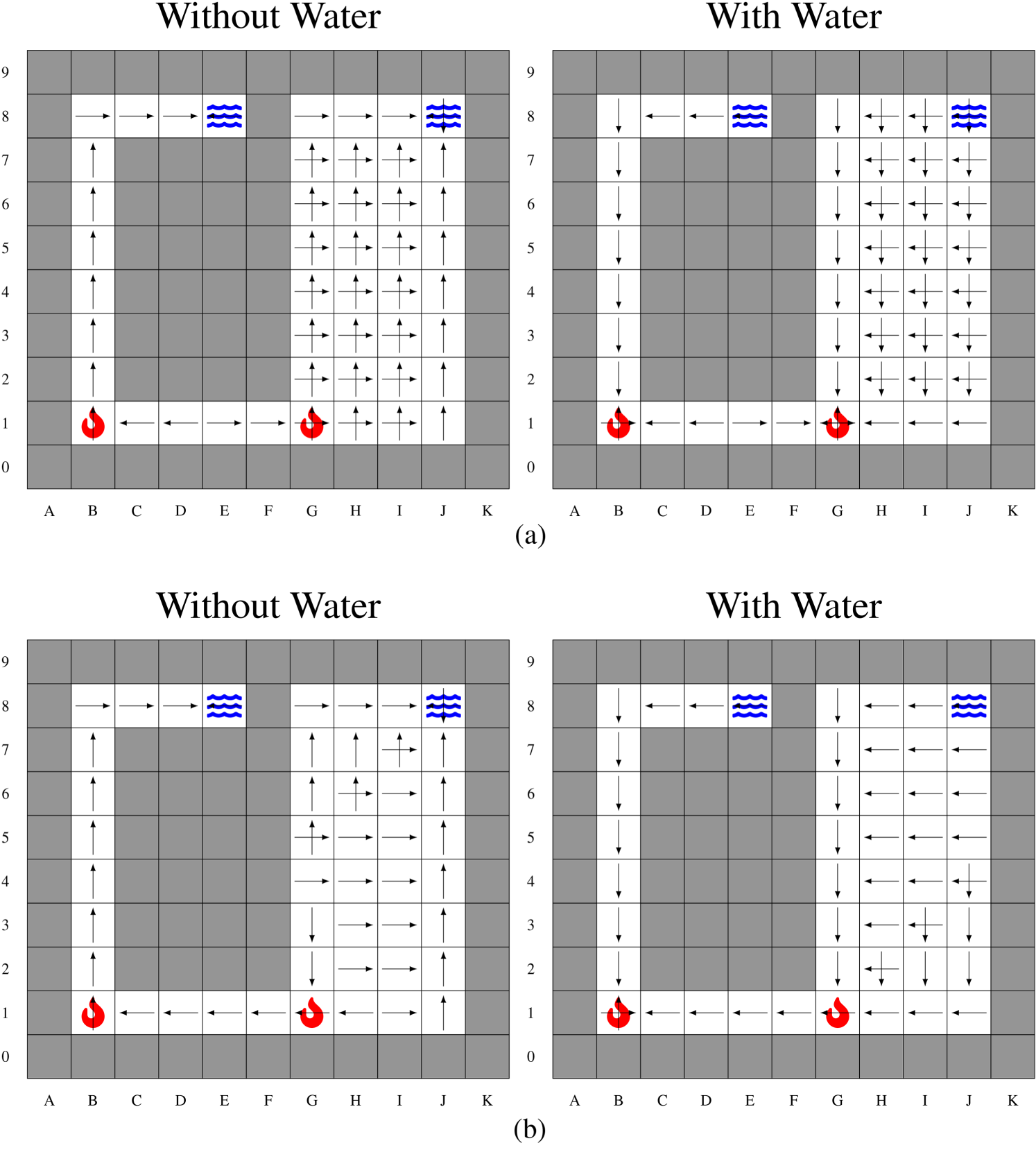
Results for Firefighter Problem F3. (a) Stochastic Policy ${\pi }_{\mathcal{m}\mathcal{d}\mathcal{p}\mathcal{-}\mathcal{s}}$ ( $\gamma =0.99$ ) and (b) Predictable Observer-Aware Markov Decision Process (pOAMDP) Policy ${\pi }_{\text{pred}}^{\mathcal{A}}$ ( $\gamma =0.99$ ).

The underlying MDPs are not SSPs anymore, so that we use $\gamma =0.99$ -discounted pOAMDPs.

Analysis of ${\pi }_{\text{pred}}^{\mathcal{A}}$

A behavior similar to the maze problem can be observed. In Figure 6, ${\pi }_{\text{pred}}^{\mathcal{A}}$ prefers the corridor over the open room. In such rooms, ${\pi }_{\text{pred}}^{\mathcal{A}}$ , as ${\pi }_{\mathcal{m}\mathcal{d}\mathcal{p}\mathcal{-}\mathcal{b}}$ (see Figure 11, page 44), tries to reach a wall and walk along it (Figures 6 and 8). In Figure 7, the pOAMDP robot tries to be more predictable by walking along the wall or by reaching Row 5 or Column F to reduce the number of optimal paths to reach the fire in the middle. In Figure 8, the pOAMDP robot prefers the fire located in $(B,1)$ and the water source located in $(E,8)$ even if another water source or fire spot is closer. This is particularly visible on the “without water” side of the figure, where ${\pi }_{\text{pred}}^{\mathcal{A}}$ always ends up going from $(G,5)$ to $(E,8)$ to refill, possibly after using the water from $(J,8)$ on the fire in $(G,1)$ once.

5. Experimenting With Humans

The objective of pOAMDP solution policies is to make it easier for an observer to predict actions or states. Of particular interest is the case of human observers. An experiment was thus conducted to confront actual human participants with stochastic and biased MDP policies ( ${\pi }_{\mathcal{m}\mathcal{d}\mathcal{p}\mathcal{-}\mathcal{s}}$ and ${\pi }_{\mathcal{m}\mathcal{d}\mathcal{p}\mathcal{-}\mathcal{b}}$ ), and with pOAMDP policies ( ${\pi }_{\text{pred}}^{\mathcal{A}}$ ). We were interested in particular in:

assessing how predictable each type of policy was for humans, by measuring the number of prediction errors;

assessing whether predictions were easy to make, by measuring their response times; and

knowing how the various robot behaviors were perceived by humans.

5.1. Protocol

Participants

Experiments have been conducted with 20 human participants (four women; aged $28.9\pm 7.7$ years) to assess the actual predictability of the three policies at hand on mazes $M_1$ – $M_7$ (Figure 4). All participants provided written consent prior to their participation.

Task

Participants were seated in front of a computer displaying a maze containing a robot and the robot’s goal. For each position of the robot, at each time step, the participant had to indicate the next action by pressing one of the four arrow keys. The robot then moved to the next position according to the policy, independently of the participant’s response, and the participant had to indicate the next action, and so on along the trajectory to the goal.

Experimental Process

Participants began with a learning phase lasting about 1 min, consisting of a maze with a random policy. Then came the test phase, consisting of three sequences of seven mazes each, each sequence associated with a policy. Participants were told that the robot’s behavior was going to change at each sequence. Each robot was identified by a color. The ordering of policies was randomized, as well as the ordering of mazes within a sequence, with the exception that $M_6$ , the largest maze, was always presented in the fourth position. These randomizations are meant to compensate for possible question order biases ² , the exception of $M_6$ being made to limit the bias in its specific case, which we wanted to prioritize in our analyses. For ${\pi }_{\mathcal{m}\mathcal{d}\mathcal{p}\mathcal{-}\mathcal{b}}$ , four different orderings over actions were used as biases (out of $4!=24$ possibilities), and each maze was randomly associated with one of them. All previously mentioned randomizations were controlled (hand-written) to prevent unwanted regularities.

At the end of each sequence (to avoid any forgetting of what he/she just experienced), the participant completed a 3-item questionnaire. For each item, the participant answered on a 7-point Likert scale from “strongly disagree” to “strongly agree.” The three items related to the policy they had just seen and were as follows: (1) this robot was easy to anticipate (Anticipation); (2) its decisions seemed generally logical (Logic); and (3) some of its decisions surprised me (Surprise). Each participant completed this questionnaire three times, once per policy. Once the test phase was over, they completed a questionnaire including: sociodemographic questions; a request to rank the three policies from easiest to most difficult, and another from most sensible to most unexpected.

On average, the experiment lasted 30 min.

Data Analysis

The data recorded during each maze were: the number of errors, that is, the number of times the next move predicted by the participant did not correspond to the move subsequently chosen by the robot; the response time (in ms), that is, from the instant when the robot finished a move to the instant when the participant indicated the position he thought would be the next. Each maze began with a two-square corridor to control the start of each trajectory, and the first square (the first response given by the participants) of each maze was removed from the analyses. One participant was removed from the analyses in Sections 5.2.1 and 5.2.2, as his response times were more than 3 standard deviations above the overall mean. Data processing on errors and response times was therefore carried out on 19 participants.

For the questionnaire, each of the three items was analyzed (Anticipation, Logic, and Surprise), see Section 5.2.3.

To determine whether there were any significant differences between the three policies, standard errors were calculated for the quantitative variables, as well as for the questionnaire.

5.2. Results

5.2.1. Numbers of Errors and Response Times

The main quantitative results are presented in Table 1, page 25, as well as in Figure 9 for errors and in Figure 10 for response times, for each policy–maze combination, plus a fake maze $\underset{i}{⨁}{M}_i$ whose results are obtained by assuming that the other mazes have been concatenated.

Figure 9.

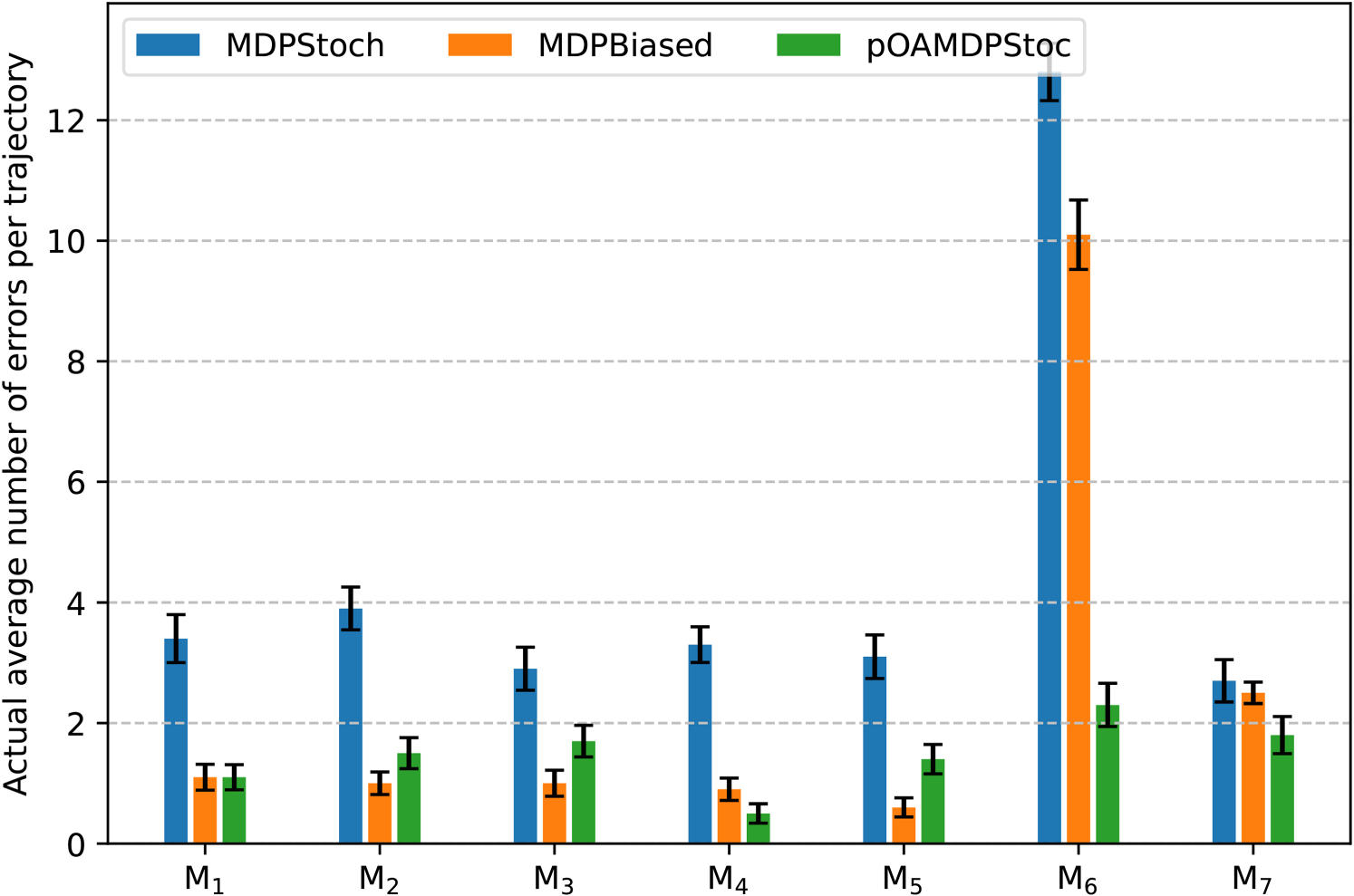
Graph Representing the Average Number of Errors Made by the Participants for Each Maze.

Figure 10.

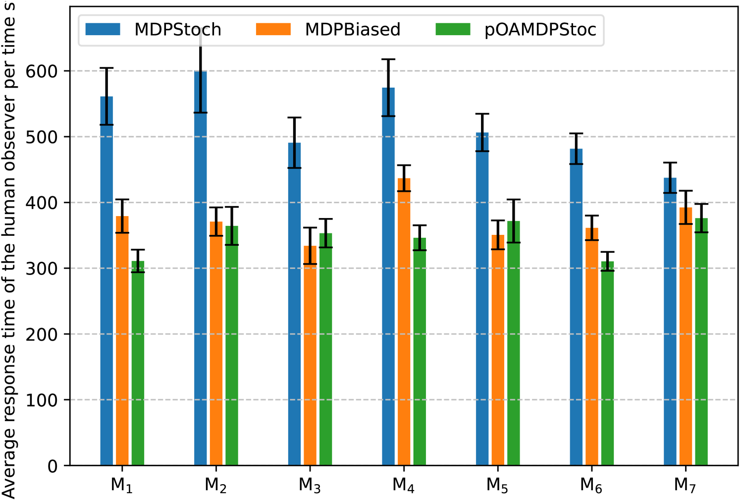
Graph Representing the Average Response Time of the Participants for Each Maze.

Figure 11.

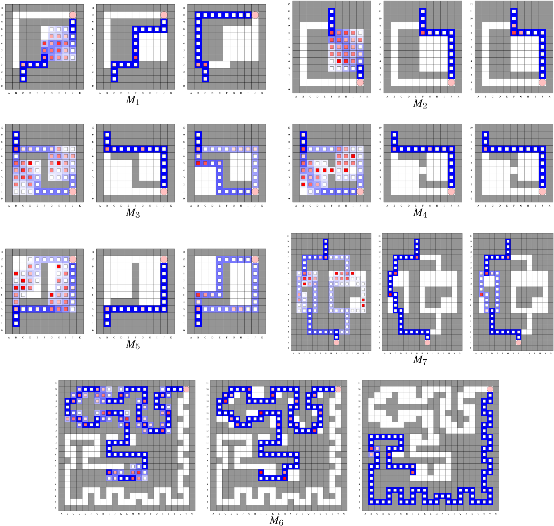
[Error Rate] Heatmaps Showing, for Each Cell, (1) [in Background] the Probability of Visit During a Trajectory from Dark Blue ( $P=1$ ) to White ( $P=0$ ), and (2) [in the Middle] the Action-Prediction Error Rate from Dark Red ( $P=1$ ) to White ( $P=0$ ). These Heatmaps are Provided for Each Maze and Each policy, from Left to Right: Stochastic MDP Policy, Biased MDP Policy, and pOAMDP Policy. Note: MDP = Markov Decision Process; pOAMDP = Predictable Observer-Aware MDP.

The first column provides the (constant) lengths of trajectories in each case as an indicator of the problem size. As anticipated, ${\pi }_{\mathcal{m}\mathcal{d}\mathcal{p}\mathcal{-}\mathcal{s}}$ and ${\pi }_{\mathcal{m}\mathcal{d}\mathcal{p}\mathcal{-}\mathcal{b}}$ generate minimal-length trajectories, while ${\pi }_{\text{pred}}^{\mathcal{A}}$ generates slightly longer ones in some cases ( $M_1$ + $M_6$ ) to follow more predictable paths.

The second column then shows the expected number of errors per trajectory according to our model ( $-V_{R_{\text{pred}}^{\mathcal{A}}}^{\pi }(s_0)$ ), which can be compared with the measured values with human observers in the third column. Values are rather similar for ${\pi }_{\mathcal{m}\mathcal{d}\mathcal{p}\mathcal{-}\mathcal{s}}$ , with typically a few more errors made by humans. Human scores are notably better than anticipated for ${\pi }_{\mathcal{m}\mathcal{d}\mathcal{p}\mathcal{-}\mathcal{b}}$ (and also better than human scores with ${\pi }_{\mathcal{m}\mathcal{d}\mathcal{p}\mathcal{-}\mathcal{s}}$ ), because humans very quickly learn the robot’s bias, which facilitates predictions in large rooms. The benefit of learning is very limited in complex mazes with many small rooms as $M_6$ . Human scores with ${\pi }_{\text{pred}}^{\mathcal{A}}$ are worse than with ${\pi }_{\mathcal{m}\mathcal{d}\mathcal{p}\mathcal{-}\mathcal{b}}$ on simple mazes (where learning biases help), but notably better on complex mazes $M_6$ + $M_7$ .

The fourth column indicates the average response time (in ms) per cell, which appears to increase with the probability of making errors. These average response times are lower for ${\pi }_{\mathcal{m}\mathcal{d}\mathcal{p}\mathcal{-}\mathcal{b}}$ and ${\pi }_{\text{pred}}^{\mathcal{A}}$ than for ${\pi }_{\mathcal{m}\mathcal{d}\mathcal{p}\mathcal{-}\mathcal{s}}$ . An important difference between response times of ${\pi }_{\mathcal{m}\mathcal{d}\mathcal{p}\mathcal{-}\mathcal{b}}$ and ${\pi }_{\text{pred}}^{\mathcal{A}}$ can be observed for $M_6$ . In this maze, it is harder for the human to learn the robot’s bias of ${\pi }_{\mathcal{m}\mathcal{d}\mathcal{p}\mathcal{-}\mathcal{b}}$ , while ${\pi }_{\text{pred}}^{\mathcal{A}}$ plans its actions to go through states with reduced action ambiguity.

5.2.2. Heatmaps

Heatmaps allow us to visualize where in the maze the participants made mistakes or were faster/slower to make a decision.

Error Rate Heatmaps

Error rate heatmaps for each maze in each policy are shown Figure 11. They are defined as follows:

the blue color represents the average number of visits computed as $\mathrm{\#}visits/\mathrm{\#}participants$ , and

the red color represents the average error rate computed as $\mathrm{\#}errors/\mathrm{\#}visits$ .

Note that, in cells with a low number of visits (light blue background color), the error rate estimate is poor compared to often-visited cells (dark blue background color). In unvisited cells (white background color), there is no error rate to estimate, hence the lack of an inner square.

The results given by the error rate heatmaps show that:

as expected, participants made many mistakes in open areas with the stochastic MDP policy;

in the pOAMDP policy, mistakes were mostly made in the beginning when participants needed to make a choice, for example, in maze $M_1$ , cell $(C,3)$ ;

in some cases, as in maze $M_1$ , cell $(B,3)$ , participants make mistakes even if there is no ambiguity over the robot’s next action. One hypothesis to explain this observation is that the participants try to anticipate the robot’s next action so that, when they make a mistake, they are likely to also make another one for the next action. This is coherent with some remarks made by the participants afterward: they anticipated the robot’s behavior over several time steps and, when the robot’s behavior did not match their expectations, they were unable to correct their predictions;

for the pOAMDP policy, participants tend to make mistakes whenever the robot changes direction. It seems that, for a human observer, changing direction is more costly than going forward;

except for maze $M_6$ (which was designed specifically to minimize the usefulness of the bias), participants perform well with the biased policy. The chosen bias for the maze problem probably facilitates human prediction a lot.

Response-Time Heatmaps

Response-time heatmaps for each maze in each policy are shown in Figure 12. The response-time heatmap is defined as follows:

the blue color represents the average number of visits computed as $\mathrm{\#}visits/\mathrm{\#}participants$ , and

the green color represents the average response time computed as $\mathrm{\#}time/\mathrm{\#}visits$ .

To make the heatmaps more readable, we cap the values to 1,000 ms, any value above 1,000 ms being indicated by a black cell. The goal of these heatmaps was to see where the participants’ decision-making was slow, if there was any kind of anticipation, and the overall response time depending on the policies.

Figure 12.

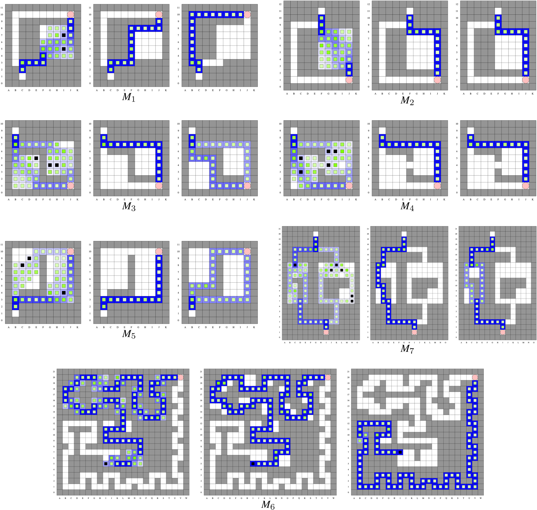
[Response-Time] Heatmaps Showing, for Each Cell, (1) [in Background] the Probability of Visit During a Trajectory From Dark Blue ( $P=1$ ) to White ( $P=0$ ), and (2) [in the Middle] the Response Time From Green (1,000 ms) to White (0 ms). These Heatmaps are Provided for Each Maze and Each Policy, From Left to Right: Stochastic MDP Policy, Biased MDP Policy, and pOAMDP Policy. Note: MDP = Markov Decision Process; pOAMDP = Predictable Observer-Aware MDP.

The response-time heatmaps show that:

in open areas, the participants take more time to make a decision;

consistent with the error heat map, for the pOAMDP policy, participants take more time to make a decision at the beginning, where they need to make a choice;

in the pOAMDP policy, we can notice that, after unexpected actions, the participants take more time for the next prediction. For example, in $M_1$ , cell $(C,3)$ , the robot action surprised the participants and their response time is higher in the next few cells. These cells also match the cells that were wrongly predicted in the error rate heatmap; and

the response time in corridors is less important, which is due to the participants’ anticipation.

Heatmaps of “Reflex” Responses

Heatmaps of “reflex” responses for each maze in each policy are shown in Figure 13. In case of a response time below 150 ms, the decision is more of a reflex, and the participant will not be able to correct his choice if needed (Henry & Rogers, 1960; Marin & Danion, 2019). These heatmaps show which portion of participants answer in <150 ms in a state. They are more precisely defined as follows:

the blue color represents the average number of visits computed as $\mathrm{\#}visits/\mathrm{\#}participants$ , and

the black color represents the rate of response times below 150 ms, computed as $N/\mathrm{\#}visits$ with $N$ the number of times a participant answers in <150 ms.

To make the heatmaps more readable, we cap the values to a 50% rate of response times below 150 ms. The goal of this heatmap was to see where humans tend to predict the robot’s action using anticipation or reflex responses. For example, when asked to predict the robot’s move in a corridor at time $t$ , some human participants might anticipate the prediction they will have to make at $t+1$ (and afterward), thus pressing keys as fast as possible along the corridor. This should result in a series of response times below 150 ms. Note that not all participants will anticipate the robot’s next move at $t+1$ , and some of them might wait for the screen to redraw the robot’s new position at $t+1$ before answering.

Figure 13.

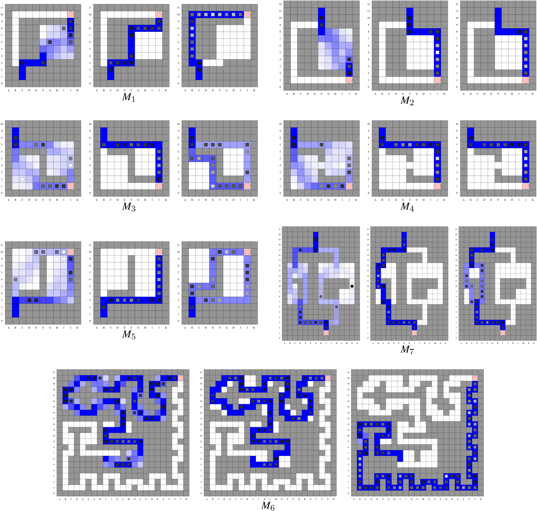
[“Reflex” Responses] Heatmaps Showing, for Each Cell, (1) [in Background] the Probability of Visit During a Trajectory From Dark Blue ( $P=1$ ) to White ( $P=0$ ), and (2) [in the Middle] the Rate of $<150$  ms Response Times From Black (Max. Rate: 50% or More) to White (Min. Rate: 0%). These Heatmaps are Provided for Each Maze and Each Policy, from Left to Right: Stochastic MDP Policy, Biased MDP Policy, and pOAMDP Policy. Note: MDP = Markov Decision Process; pOAMDP = Predictable Observer-Aware MDP.

This is also the reason why we use the 50% cap.

These response time heatmaps show that:

in rooms, most response times are above 150 ms, except along walls, either because following the wall is optimal, or because the robot is obviously going in a straight line. Note that the stochastic MDP policy has more chances to go through the center of rooms than to follow walls;

in the corridors, many participants answer in <150 ms, as can be seen in $M_1$ and in $M_2$ for example. As explained earlier, in a straight line, participants can anticipate the next action and be much faster.

5.2.3. Questionnaire and Ranking

After each sequence of mazes corresponding to a policy, participants were asked to rate this policy on a scale of 1 to 7 according to three dimensions: Anticipation, Logic, and Surprise (see Section 5.1). The average scores obtained, as well as standard errors, are shown in Figure 14. Overlapping error bars (based on standard errors) indicate no differences, while nonoverlapping error bars indicate significant differences. Concerning Anticipation, the results seem to indicate that ${\pi }_{\mathcal{m}\mathcal{d}\mathcal{p}\mathcal{-}\mathcal{s}}$ is considered more difficult to anticipate than the other two policies and that ${\pi }_{\mathcal{m}\mathcal{d}\mathcal{p}\mathcal{-}\mathcal{b}}$ is tendentially a little more difficult to anticipate than ${\pi }_{\text{pred}}^{\mathcal{A}}$ . Concerning Logic, the results seem to indicate no significant difference between the three policies, with ${\pi }_{\mathcal{m}\mathcal{d}\mathcal{p}\mathcal{-}\mathcal{b}}$ tending to be judged slightly more logical than the other two. Concerning Surprise, the results seem to indicate no significant difference between the three policies.

Figure 14.

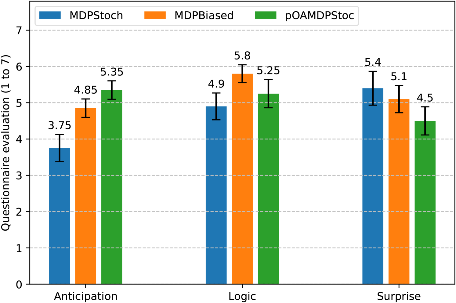
Graph Showing Questionnaire Results (Mean Score and Standard Error) on a 7-Point Likert Scale for Each of the Three Policies and for the Three Dimensions Assessed (Anticipation, Logic, and Surprise).

The results of the ranking of the three policies given at the end by the participants in terms of Anticipation and Logic are given by Table 2 (complete orderings). Note that one participant only returned a partial ordering in terms of Anticipation, hence some columns summing to 19 instead of 20. The two rankings show very similar patterns. For both Anticipation and Logic, as presented in Table 2 (score rankings), (1) ${\pi }_{\mathcal{m}\mathcal{d}\mathcal{p}\mathcal{-}\mathcal{s}}$ , which most participants consider hard to predict and even random, is typically ranked last, sometimes second, and (2) participants have a preference for ${\pi }_{\text{pred}}^{\mathcal{A}}$ over ${\pi }_{\mathcal{m}\mathcal{d}\mathcal{p}\mathcal{-}\mathcal{b}}$ .

Table 2.

Human Preferences Over Policies, Where S $={\pi }_{\mathcal{m}\mathcal{d}\mathcal{p}\mathcal{-}\mathcal{s}}$ , B $={\pi }_{\mathcal{m}\mathcal{d}\mathcal{p}\mathcal{-}\mathcal{b}}$ , and P $={\pi }_{\text{pred}}$ .

(a) Anticipation: Complete orderings
order	#votes
PBS	8
BPS	5
PSB	3
BSP	2
SBP	1
Total	19

(b) Anticipation: Score ranking
	S	B	P
1st	$1$	$7$	$11$
2nd	$5$	$9$	$5$
3rd	$14$	$3$	$3$
Total	20	19	19

(c) Logic: Complete orderings
order	#votes
PBS	8
BSP	4
PSB	3
BPS	3
SBP	2
Total	20

(d) Logic: Score ranking
	S	B	P1
1st	$2$	$7$	$11$
2nd	$7$	$10$	$3$
3rd	$11$	$3$	$6$
Total	20	20	20

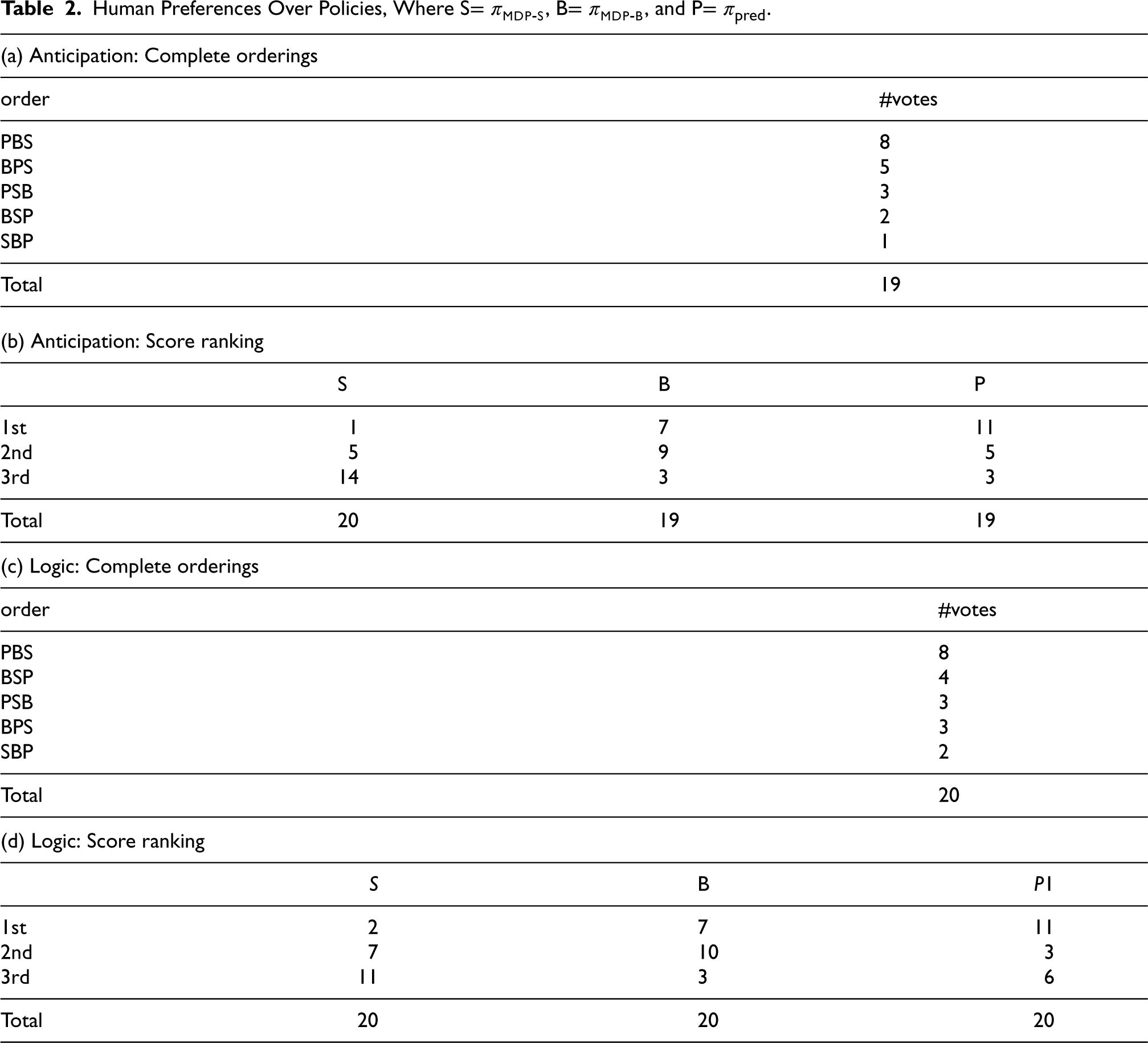
Participants often declare that the initial choice of ${\pi }_{\text{pred}}^{\mathcal{A}}$ can be surprising. This is especially the case in maze $M_6$ , and if the participants had worked with ${\pi }_{\text{pred}}^{\mathcal{A}}$ after ${\pi }_{\mathcal{m}\mathcal{d}\mathcal{p}\mathcal{-}\mathcal{s}}$ and ${\pi }_{\mathcal{m}\mathcal{d}\mathcal{p}\mathcal{-}\mathcal{b}}$ . However, despite those statements, humans still performed better with ${\pi }_{\text{pred}}^{\mathcal{A}}$ (especially in maze $M_6$ ).

5.3. Discussion

There are a few differences between the biased MDP policy and the pOAMDP policy in terms of errors, response times, and human perception, in comparison with the stochastic MDP policy, whose behavior is much harder to predict. The pOAMDP policies’ response times are better on some mazes ( $M_1$ , $M_4$ , and $M_6$ ). The pOAMDP policy induces fewer errors on more complex mazes ( $M_6$ and $M_7$ ), while the biased MDP policy induces fewer errors on mazes $M_3$ and $M_5$ , where the pOAMDP policy is not deterministic (having two possible trajectories) and where the biased MDP policy (1) turns less (on average) and (2) quickly becomes very predictable due to its bias toward the right. Subjective feedback from human participants is consistent with observed performance. The pOAMDP policy was preferred, probably because it seems easier to anticipate, while the biased MDP policy is considered slightly more logical (as it always follows the shortest paths).

The pOAMDP policy is more predictable in complex mazes such as $M_6$ , which is interesting if we want to consider more realistic scenarios. However, in less complex mazes, we do not observe significant differences between the pOAMDP policy and the biased policy. Considering more mazes such as $M_6$ in the experiment could improve the results and better emphasize the differences between the biased policy and the pOAMDP policy. The biased condition was added to this study to be able to compare the pOAMDP policy not only to a stochastic policy but also to a policy that could be easier to anticipate for the participants. We were expecting the differences between the pOAMDP policy and the biased policy to be less important than the differences between the stochastic MDP policy and the pOAMDP policy. However, the bias used for the maze was learned really fast by the participants and facilitated their predictions to the point where in certain mazes, there were not any differences between the two. A better model of a human observer would thus account for the possible biases of the robot, for example, the bias being a hidden state variable (a type in the OAMDP sense) that the observer could try to infer. This being said, a scenario that could better match the human participants’ model of the robot could be if the robot’s state were described not only by its location $(x,y)$ , but also by a direction $d\in \{\mathrm{North},South,East,West\}$ , and action set $\mathcal{A}=\{\mathrm{forward},turnRight,turnLeft\}$ , so that, without modifying the reward function, minimizing trajectory lengths will lead to prefer straight lines whenever possible.

6. Conclusion

We have introduced a new formalism, predictable observer-aware MDPs (pOAMDPs), that allows deriving policies whose next actions or next states are more predictable and proposed accounting not only for discounted problems, but also for stochastic shortest-path problems (which requires ensuring that valid solution policies can be found). With the objective of minimizing the number of prediction errors along a trajectory in an undiscounted setting, and assuming rational observer predictions, we derived two reward functions, respectively, for action and state predictability, and demonstrated that they both induce valid stochastic shortest-path problems, that is, the solution predictable policies reach terminal states with probability 1. A notable property is that the solving complexity of pOAMDPs is comparable to MDPs, thus much less than OAMDPs. In some cases, the resulting policies select counter-intuitive actions early on to increase predictability later on. The interpretation of generated policies shows significant reductions in the expected number of errors when using pOAMDP solutions on some scenarios (up to fourfold), and also benefits from using biased MDP policies, which often follow walls. The results of the experiment with human participants are consistent with these observations.

As illustrated by some benchmark problems, the proposed performance criterion can lead to less efficient policies in terms of the original performance criterion (here used only for the observer predictions). This can be addressed in various ways as, for instance, by linearly combining both reward functions, or, using constrained MDPs (Altman, 1999; Trevizan et al., 2017b), by minimizing the prediction error while constraining the value of the original criterion.

On another note, considering goal-oriented problems as we did would of course also be relevant for Miura and Zilberstein’s OAMDPs, first to determine which of their scenarios result in valid SSPs. Then, to handle SSPs with traps, that is, subsets of (nonterminal) states that cannot be escaped, an interesting direction would be to extend our work to generalized SSPs (Kolobov et al., 2011; Trevizan et al., 2017a).

Finally, we had to depart from Miura and Zilberstein’s original formalism and their static types (Miura & Zilberstein, 2021), but an important perspective is to generalize both formalisms, making for a more unified theory of observer-aware sequential decision-making. We believe that a key point to achieve this is to restrict the observer’s observability of states and actions so that the target variable, whether static or dynamic, can be a state variable, even for action predictability. What is more, this partial observability would also allow covering more real-world scenarios. In this setting, we envision looking at the continuity properties of the optimal value function to possibly propose bounding approximators and derive point-based solvers (as was done for partially observable MDPs and related models Dibangoye et al., 2016; Horák & Bošanský, 2019; Horák et al., 2017; Kurniawati et al., 2008; Pineau et al., 2006; Shani et al., 2013; Smith & Simmons, 2005; Spaan & Vlassis, 2005).