Sage Journals: Discover world-class research

Abstract

To reach a given goal, a mobile robot first computes a motion plan (ie a sequence of actions that will take it to its goal), and then executes it. Markov Decision Processes (MDPs) have been successfully used to solve these two problems. Their main advantage is that they provide a theoretical framework to deal with the uncertainties related to the robot's motor and perceptive actions during both planning and execution stages. This paper describes a navigation approach using an MDP-based planning method and Markov Localisation. The planning method uses a hierarchic representation of the robot's state space. Besides, the actions used better integrate the kinematic constraints of a wheeled mobile robot. These two features yield a motion planner more efficient and better suited to plan robust motion strategies. Also, this paper focuses on the experimental aspects related to the use of Markov Techniques with a particular emphasis on how two key elements were obtained by learning, namely the transition function (that encodes the uncertainties related to the robot actions) and the sensor model. Experiments carried out with a real robot demonstrate the robustness of the whole navigation approach.

Keywords

Autonomous Navigation Mobile Robot Markov Decision Processes Markov

1. Introduction

By design, the purpose of a mobile robot is to move around in its environment. To reach a given goal, the typical mobile robot first computes a motion strategy, ie a sequence of actions that will take it to its goal, and then executes it. Many researchers have studied these two problems since the late sixties-early seventies. In 1969, (Nilsson, 1969) introduced a planning approach based upon a graph representation of the environment whose nodes correspond to particular parts of the environment, and whose edges are actions to move from a particular part of the environment to an other. A graph search would return the motion strategy to reach a given goal. Since then, many different types of representations of the environment and many different planning techniques have been proposed (for instance, using a geometric model of the environment, motion planning computes a motion, ie a continuous sequence of positions, to move from one position to an other (Latombe, 1991)). However, the key principle remains the same: a planning stage¹ is followed by an execution stage.

The decoupling between the planning stage and the execution stage relies on the underlying assumption that the robot will be able to successfully execute the motion strategy computed by the planning stage. In most cases, this assumption is unfortunately violated, mostly because actions are non deterministic: for various reasons (eg wheel slippage), a motion action does not always take the robot where intended.

One way to solve this uncertainty problem is to address it in the execution stage: mobile robots are equipped with different sensors in order to perceive their environment and monitor the execution of the planned motion. Corrective measures are taken when required. In this framework, the first problem that a mobile robot has to solve is to localise itself. To that end, a number of localisation techniques have been proposed (Borenstein, Everett, & Feng., 1996): they are based on probabilistic models of actions and perceptions and rely on tools such as Kalman filters (Kalman, 1960; Maybeck., 1979), particle filters (Thrun, 2002), or Markov Localisation (Burgard, Fox, Hennig, & Schmidt, 1996; Fox, Burgard, & Thrun, 1998).

On the other hand, since the early nineties, approaches based on Partially Observable Markov Decision Processes (POMDP) (Bellman, Holland, & Kalaba, 1959) have been used to address the uncertainty problem in the motion planning stage. Such approaches that also rely upon a graph representation of the robot's state space provide a theoretical framework to deal with the uncertainties related to the robot's motor and perceptive actions. The output of a POMDP-based planning system is not a motion plan but rather a motion policy that gives the optimal action to perform given the belief that the robot has about its current state.

In theory, the combination of a POMDP-based planner and an execution stage relying upon a probabilistic localisation technique such as Markov Localisation (Burgard et al., 1996; Fox et al., 1998) yields a robust navigation system, ie a navigation system that does take into account the uncertainties affecting the robot so as to increase the probability to reach the goal.

Things are not that simple in practice however. The intrinsic complexity of a POMDP-based planner restricts its application to relatively simple problems (cf the complexity results establishedin (Madani, Hanks, & Condon, 2003; Papadimitriou & Tsisiklis, 1987)). Previous approaches that compute an exact optimal policy cannot handle problems with more than a few hundred states (Zhang & Zhang, 2001; Mundhenk, Goldsmith, Lusena, & Allender, 2000). Computing an approximate solution is one way to tentatively reduce the complexity but at the expense of the policy robustness (Roy, Gordon, & Thrun, 2005).

The review of the literature shows that, in practice, Markov Decision Processes (MDP) are used instead of POMDP. In MDP, the policy is computed assuming that, at execution stage, the robot knows its current state. MDPs have been successfully applied to more complex planning problem (Cassandra, Kaelbling, & Littman, 1994; Cassandra, Kaelbling, & Kurien, 1996). However, the algorithmic complexity of MDP remains high and realistic problems are likely to require too huge a number of states (Littman, Dean, & Kaelbling, 1995). To address this issue, a number of so-called aggregation techniques have been proposed. The idea is to reduce the number of states by aggregating together states that share common properties. Ref. (Dean, Givan, & Kim, 1998) for instance aggregates states sharing the same set of actions. In (Hauskrecht, Meuleau, Kaelbling, Dean, & Boutilier, 1998), a hierarchical representation of the space state is defined according to the geographic location of the states. States in the same geographic area are aggregated to obtain a set of high-level states. In a office environment for in tance, the states located in a given corridor are aggregated and define a high-level state. High level actions corresponding to transitions between high-level states are then required. In (Laroche, 2000a), partial plans are efficiently computed using a graph representation of the environment made from a topological representation of the environment. In all these methods, the aggregation of states is manually performed and is based on some a priori knowledge about the nature of the environment.

Now, in most applications, whether using aggregation techniques or not, the actions used to pass from one state to another are usually remote from the low-levelmotion commands that the robot will have to perform. It is especially true in the case where a hierarchical representation of the environment is used. Abstracting the actions yields a serious problem: how to identify the uncertainty model attached to an action? This model is essential in the computation of the optimal policy.

Characterising in a meaningful way the uncertainty corresponding to a high-level action such as “move to the next room” is next to impossible in practice. Given a robotic system, we believe it is important that the actions remains as close as possible of the low-level commands that the robot will execute. They should reflect the kinematic properties of the robot at hand. For a wheeled mobile robot for instance, the typical action sequence “rotate towards the goal, go straight and rotate again” which is used to reach a given state is not kinematically sound. A circular arc motion is more natural in the sense that it minimises wheel slippage.

MDP requires that a certain number of variables and models be characterised: what is a state? What is an action? What is the uncertainty attached to a given action? What is the uncertainty attached to the sensors? etc. In most cases, these models are given a priori (which raises the question of their validity). More interesting are the works aiming at learning these models and parameters (Koenig & Simmons, 1998; Shatkay, 1999). They usually operate in the Hidden Markov Model framework² and use the well-known Baum-Welch learning algorithm (Baum, 1972) to estimate the different parameters of the MDP model.

This paper describes a robust navigationmethod that combines a MDP-based planner along with a Markov Localisation-based execution module. It aims at solving several of the problems mentioned above with an emphasis on the applicability of the approach to real-life situations (as opposed to toy examples). To that end, a lot of effort have been put on the experimental validation of our work with an actual robot trying to perform realistic navigation tasks (which is something rarely done with MDP-based systems).

As far as MDP is concerned, our contribution is twofold: we first propose a fully automated state aggregation technique that permits to significantly reduce the number of states (and starting, to apply MDP to more realistic problems). Our aggregation technique relies upon a tool well known in Computational Geometry, the quadtree decomposition. It is important to note that this technique does not require any a priori knowledge about the structure of the state space considered. Second, for a wheeled mobile robot, we introduce actions that take into account the kinematic properties of this type of robot. Our actions results in smoother and more natural motion (that tends to minimize wheel slippage). These actions combine elementary motions for which it is possible to experimentally learn the corresponding uncertainty models. These two features yield an MDP-based planner more efficient and better suited to plan robust motion strategies.

On the experimental front, we propose a method to learn the parameters of the MDP and Markov Localisation models required. This method makes its estimation using only motors commands and raw sensor data. It requires neither a priori knowledge nor abstraction of any kind. The paper is organised as follows: The problem is stated in section 2. Section 3 describes the theoretical tools used in our navigation scheme (MDP and Markov Localisation respectively). The state aggregation method, the actions and the uncertainty model corresponding to the actions are respectively detailed in sections 4, 5 and 6. The reward function witch is a necessary part of MDP is defined in section 7. Section 8 summarises the experiments carried out with an actual robot. Finally, conclusions and future perspectives are given in section 9.

2. Statement of the Problem

As mentioned earlier, the purpose of this work is to automate the navigation of a robotic system R placed in an environment W . The ubiquitous case of a differential drive mobile robot moving in a two-dimensional workspace cluttered up with polygonal obstacles is considered. The kinematics of the differential drive mobile robot R is depicted in Fig. 1. R is equipped with two wheels whose velocity is controlled independently. Such a system is nonholonomic, meaning that R must instantaneously move in a direction perpendicular to the wheels' axle (assuming that each wheel rolls without slipping that is). It should be noted however that R can rotate on the spot (the readerinterested in the issues related to the nonholonomy problem is referred to (Laumond, 1998)).

Fig. 1.

Model of a differential drive robotic system.

Let q denote a configuration³ of R , it is defined by the triple q = (x,y,θ) with (x, y) in ℝ² the coordinates of the reference point P of R , and θ in S¹ its main orientation. The set of the possible configurations defines C, the configuration space of R . The size of R is defined as Δ_min, ie the radius of the smallest circle circumscribing R . It is assumed that R is equipped with a set of sensors (range senors typically) that return an observation of the environment. Let o denote such an observation. It goes without saying that an actual robotic system such as R is plagued with uncertainty whether it be at the control level or at the perception level. In spite of these uncertainties, the purpose of the work presented herein is to ensure that R can reach a given goal qg in a robust manner.

3. Outline of the Approach

As mentioned earlier, our robust navigation scheme combines a MDP-based planner along with a Markov Localisation-based execution module. The next two sections recall the basics of MDP and Markov Localisation respectively. The third section outlines the overall structure of our robust navigation scheme.

2.1. Markov Decision Processes

Markov Decision Processes constitute a theoretical framework to model and solve planning problems where actions are uncertain. First, we define the Markov Decision Process model and secondly we briefly introduce the algorithms generally used to solve the planning problem.

2.1.1. Definition

A Markov Decision Process (MDP) models a robot which interacts with its environment. It is defined as a 4-tuple {S, A, T, R}.

–
S is a finite set of states characterising the environment of the robot in our case. S is usually obtained by a regular decomposition of the environment or thanks to a topological map;
–
A is a finite set of actions which permits the transition between states. There is generally a discrete number of actions.
–
T:S × A × S → [0, 1] is the state transition function which encodes the probabilistic effects of actions; T(s_i, a, s_j) is the probability to go from state s_i to state s_j when action a is performed.
–
R:S → ℝ is the reward function used to specify the goal the agent has to reach and the dangerous parts of the environment. R(s) gives the reward the agent gets for being in state s.

2.1.2. Optimal Policy

In MDP, we suppose the robot knows at each instant its current state. Actions must provide all the information for predicting the next state. Once the set of states S has been defined and the goal state chosen, an optimal policy gives the optimal action to execute in each state of S in order to reach the goal state(s) (according to a given optimality criterion).

The two most important algorithms used tocalculate the optimal policy are: Value Iteration (Bellman et al, 1959) and Policy Iteration (Howard., 1960). The Value Iteration algorithm proceeds by little improvement at each iteration and requires a lot of iterations. Policy Iteration however, yields greater improvement at each iteration and accordingly needs fewer iterations, but each iteration is very expensive.

Complexity results for these algorithms can be found in (Littman et al, 1995). Each iteration is achieved in |S|³ + O(|A||S|²) for Policy Iteration and O(|A||S|²) for Value Iteration. The number of iterations needed to converge is quite difficult to determine, it seems polynomials in |S| and |A| for both algorithms (Littman et al, 1995).

3.2. Markov Localisation

In this section, we describe the method we have used to address the execution stage. To perform execution, the robot has to localise itself. The purpose of localisation is to determine the current state of the robot using its perceptive capacities and its previous actions. In order to determine this current state, we use Markov Localisation (Fox et al., 1998) that estimates the global position of a mobile robot based on its past observations and actions. More formally, let L_t be a random variable representing the state of the robot at time t, Bel(L_t = s_i) denotes the probability of the robot being in state s_i at time t knowing the observations and actions done until time : Bel(L_t = s_i) = P(s_i|o₁, …, o_t, a₁, …, a_t). Knowing Bel(L_t−1), o_t, the observation obtained and a_t, the action performed at time t, Markov Localisation permits to determine Bel(L_t) for each state $s_{i} \in S : B e l (⌈ L_{t} = s_{i} ⌉) = \frac{P (o_{t} | s_{i}) \sum_{s_{j} \in S} T (s_{j}, a_{t - 1}, s_{i}) B e l (⌈ L_{t - 1} = s_{j} ⌉)}{\sum_{s_{k} \in S} B e l ([L_{t} = s_{k}])}$ To use Markov Localisation, we need to determine P(o_t|[L_t = s_i]) called the sensor model and T([L_t−1 = s_j], a_t−1, [L_t = s_i]) that corresponds to the transition function defined in the planning stage. Typically these two elements of the Markov Localisation permits to take into account the uncertainty on the robot's observations and actions.

The initialisation of Bel(L₀) depends on the knowledge about the starting state:

–
If the starting state is known with absolute certainty: Bel(L₀) is a Dirac distribution centered at the starting state. In this case, we talk about “tracking problem”.
–
If the starting state is unknown: Bel(L₀) is a uniform distribution. We talk about “global localisation”.

Once we have computed this distribution, we choose the most probable state as the current state of the robot (if there are several states with maximum probability, one of them is selected randomly).
3.3. Navigation Scheme

The planning stage produces an optimal policy π which gives the optimal action to execute in each state of S in order to reach a goal state. The purpose of the execution stage is to ensure that the robot reaches its goal using this optimal policy. So, the execution stage has to know at each time, the current state of the robot. At each time t, Bel(L_t) is the probability distribution over the state of the environment. Using Bel(L_t), we choose the most probable state as the current state of the robot (if there are several states with maximum probability, one of them is randomly selected). Then the robot executes the action associated to this state and makes an observation. Using this new action and observation, Bel(L_t+1 = s_i) is computed for s_i. This cycle is repeated until the robot reaches the goal.

4. Definition of the Set of States

4.1. Principle

The set of states S is a discrete representation of C, the configuration space of R. Each state s_i, corresponds to a subset of C. As mentioned earlier, states are, in most cases, defined manually or, automatically, thanks to a regular discretisation of the workspace.

We propose to use the classical technique known as quadtree decomposition (Finkel & Bentley, 1974) both to automate the definition of S and optimise the number of states.

Quadtree decomposition is a hierarchical decomposition scheme that bas been used in areas as different as computer vision (Ballard & Brown, 1982), databases (Bentley, 1975), or geographic information system (C.A. Shaffer & Nelson, 1987). Its principle is illustrated in Fig. 2 for a two-dimensional space.

Fig. 2.

Quadtree decomposition principle.

It recursively divides the environment in four identical square cells. Each cell is labelled as being “free” if there is no obstacle inside, “full” if it is entirely filled with an obstacle and “mixed” otherwise. Mixed cells are divided again in four and the process goes on until a given resolution level is reached. The output of the quadtree decomposition is a hierarchical tree of free cells completed with the adjacency relationships between the cells (two cells are neighbours if they share a common edge). The number and size of the resulting cells depends on both the resolution level and the obstacles' shape.

4.2. Defining a State

The set of states is automatically defined through the combination of a quadtree decomposition of the workspace W , ie the two-dimensional xy component of C, and a regular discretisation of the θ dimension.

The workspace W is decomposed using quadtree decomposition down to a resolution level corresponding to the size Δ_min of the robotic system considered.

The quadtree decomposition of W yields a set of square cells. Each cell c_i is characterised by the coordinates (x_i, y_i) of its center and its size Δ_i, (defined as the half-length of a side of the cell). Let δ_θ denote the discretisation range of the θ dimension, it yields a finite number [2π/δ_θ] of nominal orientations.

A quadtree cell c_i and a nominal orientation θ_i define Γ_i, a three-dimensional subset of C:

Γ_{i} = {x_{i} \pm \frac{1}{2} Δ_{i}, y_{i} \pm \frac{1}{2} Δ_{i}, θ_{i} \pm \frac{1}{2} δ_{θ}}

(1)

Such a subset Γ_i defines the state s_i. In summary, a state s_i is fully characterised by its center q_i = {x_i, y_i, θ_i} and its dimensions Δ_i and δ_θ.

4.3. Reduction of the Number of States

Besides permitting the automatisation of the definition of the set of states, the main interest of the quadtree decomposition is to reduce the number of states: fewer states are required to model workspaces containing wide obstacle-free areas. In the example depicted in Fig. 3 for instance, the number of cells obtained after the quadtree decomposition is 580 (with a regular decomposition, the number of cell would be 1024).

Fig. 3.

Example of a two-dimensional workspace (left), and the resulting quadtree decomposition (right). Grey cells are partially occupied whereas black cells are fully occupied by an obstacle.

At a given resolution level, the number of cells produced by the quadtree decomposition is highly dependent on the shape and disposition of the environment's obstacles. It is therefore difficult to estimate a priori what the gain in the cell number will be. To show the interest of the approach, a statistical evaluation of the gain in the cell number was carried out. This gain was estimated with respect to two factors: the size of the environment and the size of the free space in the environment.

The results obtained are summarised in Figs. 4 and 5. In both cases, measures were established using a set of one thousand randomly-generated test environments. A test environment is computed by drawing a random number of random sized polygons.

Fig. 4.

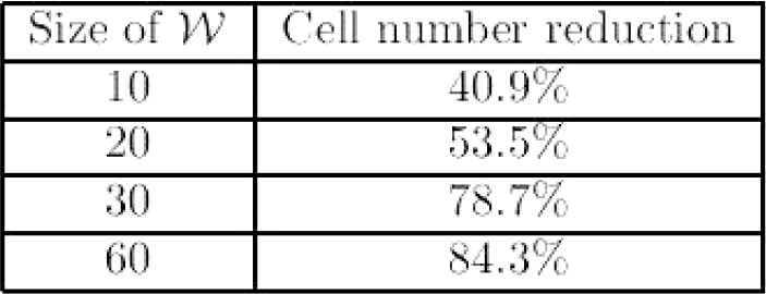
Evolution of the gain in the cell number wrt the size of the environment (expressed as n times the size of the robotic system).

Fig. 5.

Evolution of the gain in the cell number wrt the proportion of free space in the environment (for fixed-sized environments of twenty times the robot size).

These results show how significant the reduction of the number of cells can be, especially when the size of the environment grows large with respect to the size of the robotic system considered.

Of course, the gain in the cell number yields a reduction of the number of states which in turn permits to apply the MDP planning approach to bigger and more complex environments.

5. Definition of the Set of Actions

5.1. Principle

An action is the means by which the robotic system passes from one state to another. The review of the literature shows that actions are usually considered somewhat abstractedly (Cassandra et al., 1996) (Laroche, 2000b). In most cases, they do not take into account the kinematics of the robotic system at hand.

For instance, a classical action of the type “rotate towards the goal state, move straight to the goal state, and rotate again so as to reach the final orientation” is the kind of action that certainly ignores the specifics of a wheeled mobile robot whose orientation error is adversely affected by on-the-spot rotations (Fig. 6-left). Given that actions, and more importantly the uncertainty attached to them, are essential to the definition of the transition function T, we believe that they should be defined taking into account the kinematic properties of the robotic system considered.

Fig. 6.

Classical “rotate-go straight-rotate” action (left) vs Dubins action (right).

In our case, the kinematics of R, the differential drive system, is close to that of a car-like system. One way to change the orientation of R while minimising the orientation error is to move along a circular arc. Accordingly, we introduce a novel type of action: passing from one state to another is achieved through a sequence of elementary actions where an elementary action is either a straight line or a circular arc motion. Such actions are henceforth called Dubins actions as per (Dubins, 1957) that characterized similar actions for car-like systems moving forward only. An example of a Dubins action is depicted in Fig. 6-right.

5.2. Defining a Dubins Action

Given two states s_i and s_j, the Dubins action that connects them is denoted a_ij. It is defined by the collision-free Dubins path that connects q_i and q_j, ie the centers of both states s_i and s_j. The collision-free condition is met by ensuring that the path corresponding to aij remains at a distance greater than Δ_min/2 from the boundary of the cell corresponding to the union of the two cells corresponding to s_i and s_j. The isotropical growth of the boundary of this cell determines the part of the workspace W wherein the Dubins path must lie (Fig. 7).

Fig. 7.

Workspace region (in white) wherein a Dubins path must lie so as to be collision-free.

Now, because of the quadtree decomposition scheme introduced to define the states of R , the cells corresponding to two neighboring states can be significantly different in size. Their respective positions can also vary (cf §4). Accordingly, a particular Dubins action has to be defined for each cell arrangement. Fortunately, it can be done in a straightforward manner for a given cell arrangement (cf (Dubins, 1957)). Besides, the fact that the quadtree decomposition is carried out down to a given resolution level ensures that the number of cell arrangements is finite yielding thus a finite number of Dubins actions. So, this finite number is composed of a discrete set of elementary actions characterized by a finite number of lengths for straight motions and a finite number of radius sizes for circular arc motions. Fig. 6-right depicts examples of such Dubins actions. For the sake of completeness, the “rotate-go straight-rotate” action is kept to permit the transition between two states for which it is impossible to determine a proper Dubins action connecting the two. It happens for instance when two states differ only in their orientation component.

6. Definition of the Transition Function

The transition function T is central to a Markov Decision Process. It is T that encodes in a probabilistic manner the non deterministic effects of actions. Recall that T(s_i, a, s_j) is the probability to go from state s_i to state s_j when action a is executed. Clearly, T is closely related to the way the configuration error evolves when R executes a given action a. The next two sections respectively describes how the configuration uncertainty changes when R executes an action (§6.1), and how the transition function T is determined (§6.2).

6.1. Configuration Uncertainty Evolution

The knowledge that R has of its current configuration is always uncertain, ie with a limited accuracy. Classically, we have chosen a Gaussian probabilistic representation to model the configuration uncertainty (Smith & Cheeseman, 1986).

The uncertainty attached to a configuration q_k is therefore represented by its 3 × 3 covariance matrix C_k.

When R moves around, it relies upon its odometric sensors to localize itself. It is a well-known fact that odometry yields a cumulative and unbounded configuration uncertainty (the so-called drift problem (Borenstein et al, 1996)). Accordingly, the configuration uncertainty of R increases when R moves around. To model this evolution, we introduce the Uncertainty Evolution Function U that characterizes the evolution of the configuration uncertainty when R executes a given action. U(q_s, a_sg) returns the pair {q_g, C_g}, ie the nominal configuration q_g reached at the end of the action asg and the corresponding covariance C_g, assuming the uncertainty on the starting configuration q_s is null.

Giving a priori a correct characterization of U for each asg is a difficult task. The evolution of the configuration uncertainty is indeed due to the various sources of error that affect the actual robotic system R (eg command errors, wheel slippage, etc). These sources of error are very difficult to model. For this reason, we decided instead to identify U through learning. The learning procedure operates by determining the configuration uncertainty for each kind of elementary action that can compose an action, eg straight motions, circular arc motions and on-the-spot rotations. The configuration uncertainty for a given action asg is obtained by combining the configuration uncertainty of its different components. The learning procedure is detailed in section 8.3.

6.2. Defining the Transition Function

Let s_i denote an initial state and Γ_i be the corresponding three-dimensional subset of C. Let us assume that R is located at the configuration q_i = (x_i, y_i, θ_i), ie the center of Γ_i. When R executes the action a_ij, it reaches the nominal configuration, ie the center of Γ_j, corresponding to the state s_j. The covariance C_j attached to q_j is obtained thanks to the Uncertainty Evolution Function U. The pair {q_j, C_j} defines a three-dimensional Gaussian in the configuration space C of the robotic system R . In this case, ie when R is located at q_i = (x_i, y_i, θ_i), the probability T(s_i, a_ij, s_k) to go from the configuration q_i to an arbitrary state s_k when action a_ij is executed, is characterized by the integral of the Gaussian {q_j, C_j} over the subset Γ_k associated with s_k:

T (q_{i}, a_{i j}, s_{k}) = \frac{1}{α_{1}} \int_{Γ_{k}} {exp}^{- (q - q_{j}) C_{j}^{- 1} {(q - q_{j})}^{T}} d q

(2), with

α_{2} = β_{2} {(2 π)}^{3 / 2} \sqrt{det C i} .

In reality, the actual configuration of R is uncertain. Once again assuming that that the initial configuration has a Gaussian uncertainty characterized by its covariance matrix, T(s_i, a_ij, s_k) is defined as:

\begin{array}{l} T (s_{i}, a_{i j}, s_{k}) = \frac{1}{α_{2}} \int_{Γ_{i}} [{exp}^{- (q - q_{i}) C_{i}^{- 1} {(q - q_{i})}^{T}} \\ T (q_{i}, a_{i j}, s_{k})] d q \end{array}

(3), with

α_{2} = β_{2} {(2 π)}^{3 / 2} \sqrt{det C_{i}} .

A practical way to compute (3) is given in section 8.3.3.

7. Reward Function

In order to specify the goal the robot has to reach, a reward function must be specified. This reward function is defined as follows:

R (s) = {\begin{array}{l} 0 & if s is a goal \\ - 1 & otherwise \end{array}

This function is used in (Dean, Kaelbling, Kirman, & Nicholson, 1993) and (Laroche, Charpillet, & Schott, 1999). This simple reward function is sufficient and permits to distinguish the goal state from other states.

8. Experimental Results

Evaluating our navigation scheme on a real robot is an essential step to prove its efficiency and robustness. After a brief presentation of the robot, the procedures used to experimentally learn the transition function (ie the action uncertainty model), and the sensor model are described. Experimental results obtained for both the planning and the execution stages are finally presented.

8.1.
The robot we use is the Koala⁴ (Fig. 8(a)), it moves in a static known indoor environment cluttered with polygonal obstacles. It has a square size of approximately 30 per 30 centimeters. It has six wheels differentially driven. It is equipped with sixteen infrared proximity sensors (Fig. 8(b)). These sensors have a very limited range of perception: they detect obstacles in front of them at a distance of about fifteen centimeters, and within a field-of-view of ten degrees. The sensors' response is very noisy further reducing their reliability. Let us note how navigating such a robot is challenging as far as uncertainty is concerned: its sensory equipment is really poor and the uncertainty attached to its motions is high because of its wheels configuration (high wheel slippage).

Fig. 8.
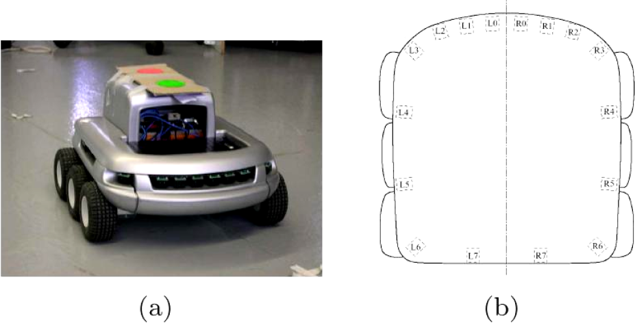
The Koala robot and the infrared sensors layout.
8.2. Experimental Set-Up for Learning Transition Function

To perform learning, we need to accurately know the configuration of the robot when it moves in its environment. To determine this configuration, we have used a camera placed on the ceiling and two coloured reference marks placed on the Koala to track its actual configuration (Fig. 9). Using colour filters on camera's images, the centres of the two coloured marks are detected with high accuracy and an homography is applied to obtain the robot's configuration (it was obtained with a 2 millimeter error margin).

Fig. 9.

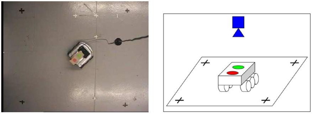
Experimental set-up used to learn the transition function.

8.3 Learning the Transition Function

We have seen the importance of the transition function T: it encodes in a probabilistic manner the non-determinist effects of the actions performed by the robot (cf section 6). In order to apply our method on the Koala, we need to compute this function according to the Koala's motion uncertainties.

To begin with, the configuration uncertainty for each elementary action is obtained by learning. To do so, we have defined an experimental set-up to perform this learning. Then, combining the uncertainty model of the different elementary actions composing a given Dubins action, we can obtain its uncertainty model. Finally, the transition function T is computed for a specific action and a specific initial state according to the configuration uncertainty of the action. This method provides a transition function for every Dubins actions and any initial state according to the displacement uncertainty of the Koala.

8.3.1. Uncertainty Evolution Function for Elementary Actions

The purpose of the learning step is to measure and model the uncertainty of the actions executed by the Koala, in particular the configuration uncertainty of elementary actions (cf section 6.1). For each elementary action a, we have to learn the Uncertainty Evolution Function U(q_s, a) which returns the pair {q_g, C_g} ie the nominal configuration q_g reached after action a and the corresponding covariance matrix C_g.

To estimate the pair {q_g, C_g}, we collect experimental data. For each elementary action a, we let the robot perform this action several times. For each run, knowing exactly the initial configuration q_s, we measure the exact configuration after the action is done (using our camera system). With those measures, we can compute the average and the covariance {q_g, C_g} of this data to obtain the Uncertainty Evolution Function U_a for the elementary action considered. Fig. 10(b) depicts an example of the Uncertainty Evolution Function U_a obtained for a particular circular arc motion a shown on Fig. 10(a).

Fig. 10.

Example of an elementary action a (right) and the the associated Uncertainty Evolution Function obtained through learning (left).

8.3.2. Uncertainty Evolution Function for Dubins Actions

The Uncertainty Evolution Function U_a for a given Dubins action a is obtained in a straightforward manner by combining the Uncertainty Evolution Function of each elementary action composing it. More precisely, for a Dubins action a composed of n elementary actions we have U(q_s, a) = {q_g, C_g} where q_g is the configuration reached by the final elementary action of a, and C_g is the covariance matrix defined as:

C_{g} = \prod_{k = n}^{2} C_{k}^{T} C_{1} \prod_{k = n}^{2} C_{k}

(4)

The learning stage duration is reduced since we just need to perform learning of elementary actions to obtain uncertainty model of all actions.

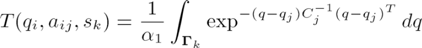
8.3.3. Computation of the Transition Function

Given the Uncertainty Evolution Function for an action a_ij and the initial state s_i of the robot, we have to compute for all states s_k ∈ S the transition function T(s_i, a_ij, s_k). We proceed as follow:

A set of one hundred configurations is randomly drawn in si. This draw is performed according to a Gaussian distribution defined by {q_i, C_i} with C_i selected as a function of the cell width. It permits to model the uncertainty on the configuration in the initial state before the action is done.

For each drawn configuration in si, we randomly draw a large set of configuration samples (about one thousand samples) according to the result {q_j, C_j} of the Uncertainty Evolution Function of a_ij.

Finally, the probability for R to reach a specific state s_k, after a_ij is performed, is given by the number of drawn configurations in the subset Γ_k corresponding to s_k (normalized wrt the total number of samples).

Figure 11 illustrates the computation principle for one drawn configuration in si (depicted by the cross): using the Uncertainty Evolution Function of a_ij (depicted by the ellipse), a large set of configurations is drawn (depicted by the points) and by counting the number in each state we obtain the probability to reach it after the action is done. Thus, we obtain the probability of reaching any state after the action ay is performed by the robot from state s_i.

Fig. 11.

Illustration of the Transition Function computation

8.4. Learning the Sensor Model

To use Markov localization, it is necessary to define a sensor model in order to obtain P(O_t|[L_t = s_i]) (the probability of doing the observation O_t knowing that the robot is in state s_i at time t).

The Koala is equipped with sixteen infrared proximity sensors, so a Koala's observation corresponds to the data of these sixteen sensors and O_t is a sixteen dimensional vector. A sixteen dimensional Gaussian has been selected to model the sensor model associated to each state. The next two sections describe in detail how the learning of this Gaussian is done for each state.

8.4.1. Typical States

Performing the learning for each states of S with a real robot is impossible when the number of states becomes important. It turns out however that a lot of states are similar with respect to the obstacles that surround them. This property allows us to define so-called typical states (Fig. 12). The number of typical states depends on the environment's size and on the resolution level of the quadtree decomposition. Let N be the resolution level of the quadtree decomposition, the upper bound of the number of typical states is $8 \times \sum_{l = 0}^{N} (2^{k} + 4)$ and the maximum number of states (corresponding to a regular decomposition) is 8 × 2^2N. Thus when N increases, the maxi mum number of typical states becomes less than the maximum number of states. So, we reduce the duration by performing the learning only on the set of typical states.

Fig. 12.

Examples of typical states

8.4.2. Experimental Set-Up

To learn the sensor model using the robot in the real environment, we follow this procedure for each typical states_t:

For a given number No of iterations (approximately one hundred):

The robot is randomly placed in γ_t;

For each configuration, an observation O_t is recorded.

A sixteen dimensional Gaussian is defined according to the obtained data. The average vector μ_O and the covariance matrix C_O are computed using the classical formulas: $μ_{O} = \frac{\sum_{t = 1}^{N_{O}} O_{t}}{N_{O}}$ and $C_{O} = \frac{\sum_{t = 1}^{N_{O}} (O_{t} - μ_{O}) \cdot {(O_{t} - μ_{O})}^{T}}{N_{O}}$ .

By defining the sensor model using the real environment and the real robot, we ensure it will match the reality during execution step.

8.5. Planning Results

Figs. 13 and 14 show two plans generated using our method. On these plans, full cells are in black, free cells in white and mixed cells in grey. The goal corresponds to the crossed cell. Each light grey arrow represents an on-the-spot rotation. Dubins actions are represented by black segments and circular arcs (with arrowheads attached to show the orientations).

Fig. 13.

Plan for 464 states (58 cells, 8 orientations) computed with Value Iteration in 7s.

Fig. 14.

Plan for 144 free states (18 cells, 8 orientations) computed with Value Iteration in 45 s.

When the plan is computed, we assign to each state an action which is the optimal action in order to reach the goal. The discretization range δ_θ of the θ dimension is chosen to be π/4. Thus, it yields eight nominal orientations. So, on the plan, we have eight states for one cell, thus there is eight actions per cell. Each action corresponds to the optimal action for one state.

On these figures, we can see that the main feature of MDP is kept: uncertainty on the action is integrated in the planning process. Indeed, safe actions are chosen: there are on-the-spot rotations and simple Dubins actions (like single translations or large circular arc motions). In these cases, the large number of on-the-spot rotations is induced by the environment's size. Indeed, the state definition produces small states and thus few complex Dubins actions can be performed.

Fig. 15 shows the optimal path extracted from a plan. It illustrates how smoother paths are obtained, especially when the robot has to cross a large free space. Because of the quadtree decomposition that yields large cells and the Dubins actions, the final motion obtained is not a lengthy sequence of short translations and rotations on spot. It features instead a few long circular or straight line motions. Furthermore, smoother path means a reduced uncertainty on the final configuration.

Fig. 15.

Optimal path extracted from a plan for 608 free states (76 cells, 8 orientations).

8.6. Execution Results

In this section, we show an example of execution using our approach. In this example, the Koala evolves in the static environment depicted in Fig. 16(a), and its goal is to reach the grey cell.

Fig. 16.

Execution steps at times t = 0 (left) and t = 1 (right)

Here, we are interested in a problem in which we suppose that the robot does not know its starting configuration, ie a global localization problem.

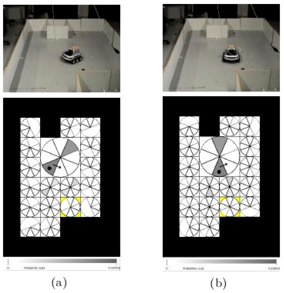
During execution we show, after each time the robot has done an observation, the real position of the robot (given by a photo) and the distribution Bel(L_t) over the set of state. So, the probability Bel([L_t = s]) which represents the robot's belief that it is in a state s at time t is depicted by a pie chart included in c and covering the range ori (hence we have eight slices in a cell because we consider eight subranges of possible orientations). The colour of a slice depends on the value of Bel([L_t = s]): the highest the probability is, the darkest it is represented. For more details, a scale is given below each environment's representations (this scale depends on the best probability we have). Also, if there are no slices corresponding to a state, this mean that the probability of being in this state is null. The state chosen to be the current state of the robot (among the states with maximum probability) is shown with a black spot and the optimal action attached to it is represented by a black arrow, and was obtained using the optimal policy. The policy computed for our environment is given in Fig. 14. Below, we describe in detail an execution in this environment and Fig. 16, 17, 19, 20 depict the different steps of this execution.

Fig. 17.

Execution steps at times t = 2 (left) and t = 3 (right)

Fig. 18.

Execution steps at times t = 4 (left) and t = 5 (right)

Fig. 19.

Execution steps at times t = 6 (left) and t = 7 (right)

Fig. 20.

Execution steps at times t = 8 (left) and t = 9 (right)

At time t = 0, before the first observation, the robot is put in an arbitrary configuration (Fig. 16(a)), and the distribution Bel(L₀) is set to uniform. The goal cell is depicted in light grey. Then at time t = 1 a first observation is made and Bel(L₀) is updated to obtain Bel(L₁). The robot perceives a wall on its front right and nothing else around (Fig. 16(b)). So, it does not know exactly where it is, but it believes that it should be in state corresponding to this observation. The current state among the high-probably states is chosen to be the high probably state at the bottom left. So, the robot will perform the optimal action (a rotation on the spot to the left depicted by the dark arrow) attached to the current state, according to optimal policy (Fig. 14).

From time t = 2 to time t = 4, the robot has done rotations on the spot and has made new observations. Thus its belief has been updated according to both action and sensor models. At time t = 3 the observation does not match very well the action model: it knows that it has done a rotation, but the sensors indicates a wall at its right. Because of its arbitrary starting orientation, its actual orientation is not perfectly known, so different states match this observation. But at time t = 4, the observation done and the action applied confirm its real configuration: it believes that there is a wall on its back. At time t = 5 the robot is in the whole place and its sensors can't sense any obstacle due to their short range of perception. It does not know if it comes from East or West. At this time, the real configuration of the robot corresponds to its believes, but it is not on the center of the big cell, it is on the South border of this cell oriented to the West.

From time t = 6 to time t = 8 it continues to execute actions and to update its belief knowing it is still in the centre of the environment. And finally at time t = 9, it has performed the action and made an observation that it is front of a wall. Knowing it was somewhere in the whole space of environment facing the South-East, and it has now a wall on front of it, it is sure at 71 percent that it has reached the goal. The execution is a success since it has really reached the goal.

Several experiments were carried out with our robot. In most cases, the execution runs in which the robot knew its initial state proved successful (except in situations where, because of the symmetries occurring in the environment, the robot could not disambiguate its current state). The success rate when the robot did not know its initial state was less important but remained satisfactory giving the robot at hand and the quality (or lack thereof) of its sensory equipment.

9. Conclusion and Perspectives

This paper has described a robust navigation method that combines a MDP-based planner along with a Markov Localization-based execution module.

As for the MDP-based planner, we propose to reduce the state space through the use of a hierarchic representation of the robot's environment. This hierarchic representation, based on a quadtree decomposition, has one main advantage: it automatically defines the set of states and so no assumption or a priori knowledge about the robot's environment is needed. We also propose to use smoother actions that better integrate the kinematic constraints of a wheeled mobile robot. These two features yield a motion planner more efficient and better suited to plan robust motion strategies.

For both the planning and execution stage, the learning of the transition function and the sensor model has allowed the implementation of our approach on a real robotic platform. Experimental results, carried out with a challenging platform have demonstrated the validity and the robustness of our navigation scheme.

The next step of this work is to develop replaning of actions. In the planing stage, we suppose that actions start in the middle of a state and stop in the middle of another state (this is the assumption made in MDP), in practice this is not the case. The purpose would be to modify this action during execution, in function of perception, so that an action starting anywhere in a state, stopping as close as possible in the middle of the stop cell.

Footnotes

1

In reactive systems, the planning stage amounts to very little.

2

Hidden Markov Model are close to MDP except that they do not include actions.

3

The configuration of a robotic system is a set of independent parameters that uniquely defines the position and orientation of every point of the system.

4

References

Ballard

, & Brown

(1982). Computer Vision. Prentice–Hall, Englewood Cliffs, NJ.

Baum

L. E.

(1972). An Inequality and Associated Maximization Technique in Statistical Estimation for Probabilistic Functions of a Markov Process. Inequalities, 3, 1–8.

Bellman

Holland

, & Kalaba

(1959). On an Application of Dynamic Programming to the Synthesis of Logical Systems, Vol. 6. ACM Press.

Bentley

J. L.

(1975). Multidimensional Binary Search Trees Used fro Associative Searching. Communications of the ACM, 19, 509–517.

Borenstein

Everett

, & Feng

(1996). Navigating Mobile Robots: Systems and Techniques. Kluwer Academic Publishers. A. K. Peters, Ltd., Wellesley, MA.

Burgard

Fox

Hennig

, & Schmidt

(1996). Estimating the Absolute Position of a Mobile Robot Using Position Probability Grids. In AAAI/IAAI, Vol. 2, pp. 896–901.

Shaffer

C.A.

Shaffer

H. S.

, & Nelson

(1987). QUILT: A geographic information system based on quadtrees. Tech. rep., University of Maryland.

Cassandra

A. R.

Kaelbling

L. P.

, & Kurien

J. A.

(1996). Acting under uncertainty: Discrete Bayesian models for mobile robot navigation. In Proceedings of IEEE/RSJ International Conference on Intelligent Robots and Systems.

Cassandra

A. R.

Kaelbling

L. P.

, & Littman

M. L.

(1994). Acting Optimally in Partially Observable Stochastic Domains. In Proceedings of the Twelfth National Conference on Artificial Intelligence (AAAI-94), Vol. 2, pp. 1023–1028 Seattle, Washington, USA. AAAI Press/MIT Press.

10.

Dean

Givan

, & Kim

K.-E.

(1998). Solving Stochastic Planning Problems with Large State and Action Spaces. In Artificial Intelligence Planning Systems, pp. 102–110.

11.

Dean

Kaelbling

L. P.

Kirman

, & Nicholson

(1993). Planning With Deadlines in Stochastic Domains. In Prooceedings of the 11th National Conference on Artificial Intelligence, pp. 574–579.

12.

Dubins

L. E.

(1957). On curves of minimal length with a constraint on average curvature, and with prescribed initial and terminal positions and tangents. AJM, 79, 497–517.

13.

Finkel

, & Bentley

(1974). Quad trees: a data structure for retrieval on composite keys. Acta Inform., 4, 1–9.

14.

Fox

Burgard

, & Thrun

(1998). Active Markov Localization for Mobile Robots. In Robotics and Autonomous Systems, Vol. 25, pp. 195–207.

15.

Hauskrecht

Meuleau

Kaelbling

L. P.

Dean

, & Boutilier

(1998). Hierarchical Solution of Markov Decision Processes using Macro-actions. In Uncertainty in Artificial Intelligence, pp. 220–229.

16.

Howard

R. A.

(1960). Dynamic Programming and Markov Processes. MIT Press, Cambridge, Massachussets, U.S.A.

17.

Kalman

(1960). A new approach to linear filtering and prediction problems. Trans. Of the ASME, Journal of basic engineering, 82, 35–45.

18.

Koenig

, & Simmons

(1998). Xavier: A Robot Navigation Architecture Based on Partially Observable Markov Decision Process Models. MIT Press.

19.

Laroche

Charpillet

, & Schott

(1999). Mobile robotics planning using abstract markov decision processes. In IEEE International Conference Tools with Artificial Intelligence.

20.

Laroche

(2000a). Building Efficient Partial Plans using Markov Decision Processes. In 12th IEEE International Conference on Tools with Artificial Intelligence (ICTAI'00).

21.

Laroche

(2000b). Processus D'ecisionnels de Markov appliqu'es la planification sous incertitude. Ph.D. thesis, Universitée Henri Poincaré Nancy.

22.

Latombe

J.-C.

(1991). Robot Motion Planning. International Series in Engineering and Computer Science; Robotics: Vision, Manipulation and Sensors. Kluwer Academic Publishers, Boston, MA, U.S.A. 651 pages.

23.

Laumond

J.-P.

(Ed.). (1998). Robot motion planning and control, Vol. 229 of Lecture Notes in Control and Information Science. Springer.

24.

Littman

M. L.

Dean

T. L.

, & Kaelbling

L. P.

(1995). On the complexity of solving Markov decision problems. In Proceedings of the Eleventh Annual Conference on Uncertainty in Artificial Intelligence (UAI–95), pp. 394–402 Montreal, Quebec, Canada.

25.

Madani

Hanks

, & Condon

(2003). The undecidability of probabilistic planning and related stochastic optimization problems.

26.

Maybeck

P. S.

(1979). Stochiastic Models, Estimation, and Control, Volume 1. Academic Press, Inc.

27.

Mundhenk

Goldsmith

Lusena

, & Allender

(2000). Complexity of finite horizon Markov decision process problems. J. ACM, 47(4), 681–720.

28.

Nilsson

N. J.

(1969). A Mobile Automaton: An Application of Artificial Intelligence Techniques. In Proc. of the 1st IJCAI, pp. 509–520 Washington, DC.

29.

Papadimitriou

, & Tsisiklis

J. N.

(1987). The complexity of Markov decision processes. Math. Oper. Res., 12(3), 441–450.

30.

Roy

Gordon

, & Thrun

(2005). Finding Approximate POMDP solutions Through Belief Compression. Journal of Artificial Intelligence Research, 23, 1–40.

31.

Shatkay

(1999). Learning Hidden Markov Models with Geometrical Constraints. In Uncertainty in Artificial Intelligence, pp. 602–611.

32.

Smith

R. C.

, & Cheeseman

(1986). On the representation and estimation of spatial uncertainty. Int. Journal of Robotics Research, 5(4), 56–68.

33.

Thrun

(2002). Particle filters in robotics. In Proceedings of the 17th Annual Conference on Uncertainty in AI (UAI).

34.

Zhang

, & Zhang

(2001). Speeding Up the Convergence of Value Iteration in Partially Observable Markov Decision Processes. JAIR, 14, 29–51.

Robust Navigation using Markov Models

Abstract

Keywords

1. Introduction

2. Statement of the Problem

2.1. Markov Decision Processes

2.1.1. Definition

3.2. Markov Localisation

4. Definition of the Set of States

4.1. Principle

5.1. Principle

6.1. Configuration Uncertainty Evolution

6.2. Defining the Transition Function

8. Experimental Results

8.3.1. Uncertainty Evolution Function for Elementary Actions

8.4.1. Typical States

8.5. Planning Results

Footnotes

1

2

3

4

References