Sage Journals: Discover world-class research

Abstract

This paper presents exact local interpretable model-agnostic explanation (ELIME) algorithm for explainable machine learning, which provides a comprehensible explanation of the decision-making process and predictions of machine learning models. Building upon existing model-agnostic interpretation methods, our approach enhances feature importance evaluation through single-feature sensitivity analysis and introduces a weighted distance metric based on sensitivity values. This sensitivity information is utilized for both calculating distances and generating training data for model fitting, improving the quality and reliability of the explanations. The enhanced ELIME algorithm is particularly effective for tabular classification domains, offering explanations that closely resemble the decision boundaries of the model. Comparative analysis with local interpretable model-agnostic explanation (LIME), deterministic LIME (DLIME), and active learning-based DLIME (AL-DLIME) demonstrates that while ELIME achieves superior fidelity and accuracy compared to DLIME and AL-DLIME, its stability is lower. However, ELIME outperforms LIME across all three metrics.

Keywords

explainable artificial intelligence machine learning interpretability model-agnostic interpretation black-box models

1. Introduction

The reliability and safety of machine learning models are especially crucial because they have been gradually applied to safety-critical fields including medical diagnostics (Kermany et al., 2018; Shinde, 2023), autonomous driving (Morooka et al., 2023), and airplane collision avoidance systems (Julian et al., 2019; Manfredi & Jestin, 2016). However, because they contain a large number of nonlinear internal relations, models such as convolutional neural networks (CNN) and deep neural networks are typically viewed as “black boxes” (Hassija et al., 2024; Minh et al., 2022), making it difficult for humans to intuitively understand the model’s decision-making process, and providing no means of knowing the model’s learning outcomes. This makes the machine learning model noninterpretable and further impedes human understanding of the model’s decision-making process, as well as their trust in the prediction results of the model (Van der Velden et al., 2022).

Therefore, constructing human-understandable explanations for machine learning models is critical to their safety and reliability (Longo et al., 2024; Mersha et al., 2024). Transparency can be improved by explaining the model’s predicted results. Potential misclassification and anomalous model behavior can be detected and improved, enhancing model safety. Explainable machine learning can improve the model’s credibility, which can help humans understand the model’s decision-making process and behavioral patterns. In the end, humans will be able to trust and accept the prediction results made by the model, thereby enhancing its reliability (Yang et al., 2022).

The model-agnostic approach to interpretation aims to develop a generalized algorithm that can explain any model so that it can be applied to provide explanations for various types of machine learning models (Henckaerts et al., 2022). As shown in Figure 1, the model predicts that the patient has influenza, and the explanatory model gives an explanation for this prediction based on the patient’s condition. According to the explanation, “sneezing” and “headache” are considered by the explanation model to support the prediction of influenza, while “no fatigue” is considered to be opposing. With the explanations, humans know the basis for the model’s predictions and can make an informed decision about whether to believe the model’s predictions (Dwivedi et al., 2023).

Figure 1.

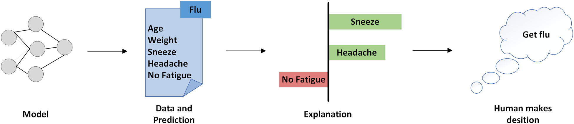
An example of a model-agnostic interpretable methods.

Local interpretable model-agnostic explanation (LIME; Ribeiro et al., 2016) is a well-known model-agnostic algorithm based on instances. To make local perturbation samples, the method randomly disrupts instances. It then fits the prediction results of the perturbation samples to a linear model, producing model-independent explanations for the instances that require interpretation. LIME has been applied to the medical field many times, for example, for interpreting intensive care data (Katuwal & Chen, 2016) and cancer data (Moreira et al., 2020; Zhang et al., 2018). However, LIME lacks stability, and stability is crucial for the model’s interpretation results, especially in the medical field (Kaur et al., 2021), where instability erodes confidence in the interpretation.

A method based on LIME is called deterministic LIME (DLIME; Zafar & Khan, 2021). The method uses agglomerative hierarchical clustering (AHC) to classify the dataset into different clusters (Li et al., 2022) and uses the K-nearest neighbor (KNN) classifier to find the data that is closest to the instance to be interpreted. To train a simple model to generate explanations, all of the data in the cluster where that data is located is selected. Although the DLIME explanation results are more stable when random perturbations are removed, this process also makes the explanation results highly dependent on the distribution of samples in the dataset. There may be significant differences in the fidelity and accuracy of the interpretations obtained from different instances to be interpreted.

Building upon DLIME, active learning-based DLIME (AL-DLIME; Holm & Macedo, 2023) further enhances the model’s interpretability. The method has two main objectives: avoiding the nondeterminism of LIME to ensure more stable explanations, and training the surrogate model with a restricted selection of instances, which is particularly useful in domains where labeled data is scarce. AL-DLIME provides a comprehensive comparison between LIME and DLIME, focusing on model performance and faithfulness to the underlying black box models, while maintaining the quality of generated explanations in terms of accuracy, consistency, and faithfulness.

In conclusion, LIME suffers from the problem of unstable interpretation results, even if it offers a sound thinking paradigm for model-agnostic interpretability. DLIME and AL-DLIME improve stability by clustering, but the fidelity and accuracy of the interpretation results remain to be proven, as other data instances in the dataset can differ significantly from the instances needed to be interpreted.

In order to improve the fidelity and accuracy of interpretation results, exact LIME (ELIME) is proposed. ELIME incorporates single-feature sensitivity analysis to calculate sensitivity values, which are then used to weight the features in a weighted Euclidean distance metric. This approach allows for a more nuanced similarity measurement. Additionally, ELIME generates training data based on these sensitivity values to improve the quality of the explanations. This method aims to provide explanations that closely approximate the decision boundary of the original model, achieving superior fidelity and accuracy compared to DLIME and AL-DLIME.

The main contributions of this paper are as follows: (1)

We introduce the concept of single-feature sensitivity analysis to evaluate the impact of each feature on model predictions. These sensitivity values are used as weights in a weighted Euclidean distance metric to enhance the accuracy of similarity measurements.

(2)

We generate training data based on sensitivity results, allowing for interpretation results that more closely approximate the local decision boundary of the model.

(3)

We conduct comprehensive experimental evaluations using established metrics (stability, fidelity, and accuracy) to validate the effectiveness of our method, demonstrating its superiority through comparative analysis.

2. Related Work

An important indicator of an explanation method’s classification is whether it is related to the model type (Kaur et al., 2022). Depending on whether they make use of information regarding the internal parameters of the model, explanation methods can be categorized into two types: both model-agnostic and model-related.

2.1. Model-Related Explanation Methods

The deep interpretation technique used in the model-related explanation method is a white-box-based method for interpreting machine learning models using known model architectures, parameters, and training data. The representative algorithms of this technique are class activation mapping (CAM; Zhou et al., 2016), gradient-weighted CAM (Grad-CAM; Selvaraju et al., 2020), and so on.

CAM is a model-related interpretation method for interpreting CNN models. CAM is based on the linear relationship between the classification output layer and the convolutional layer of the previous layer, and through the overall average pooling operation, the weights related to the categories of the prediction results are linearly superimposed on the activation maps of the convolutional layer, and the final activation maps of the prediction results are generated, which use heat maps to highlight the most relevant content in the input images.

Grad-CAM improves upon CAM. To generate a highlighted heat map, Grad-CAM utilizes backpropagation techniques, where the signals backpropagated to the convolutional layers are used as weights, and then the picture feature convolutional layers are linearly superimposed.

2.2. Model-Agnostic Explanation Methods

Using a black-box model, this model-agnostic explanation method figures out what something means by examining provided inputs and outputs. It does not need any data from inside the model, such as the network structure and parameters (Lundberg & Lee, 2017).

Among the most representative model-agnostic interpretation techniques is LIME, or the model-agnostic locally interpretable method. By randomly perturbing the input instances, LIME generates samples of perturbations. It then predicts each sample of perturbations using the model to be explained. Finally, it performs linear regression on these predictions to generate explanations, establishing a relationship between the input variables and the predictions to demonstrate the model’s explanation of the predictions for individual instances.

DLIME is an improvement to LIME in the tabular domain. DLIME uses AHC of the data within the training set and then uses the KNN method to select the cluster in which the instances are located and uses the samples within that cluster as perturbation samples instead of the randomly generated perturbation samples in LIME, and then performs linear regression on the instances within the cluster to generate explanations.

Building upon DLIME, AL-DLIME introduces an active learning strategy to optimize instance selection. By carefully choosing the most informative samples for training the surrogate model, it reduces the dependency on large amounts of labeled data. While this approach successfully improves the stability of explanations compared to DLIME, experimental results suggest that there might be tradeoffs between stability and other performance metrics such as fidelity and accuracy across different types of datasets.

3. ELIME Framework

ELIME enhances the interpretability of black-box models through feature sensitivity analysis and critical value-based sampling. The implementation flow is shown in Figure 2.

Figure 2.

Exact local interpretable model-agnostic explanation (ELIME) flowchart.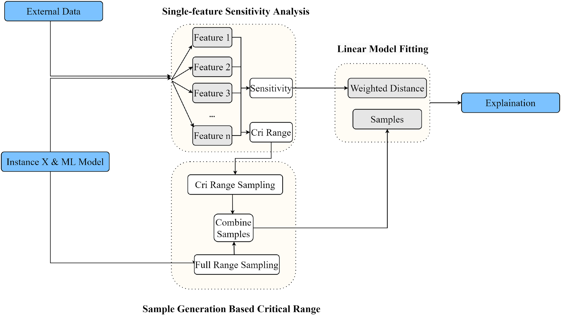

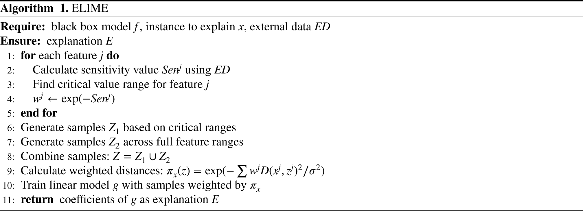
For each feature, ELIME performs sensitivity analysis by varying the feature value while keeping other features constant (Algorithm 1 Steps 1 and 2). The analysis uses the test set data distribution to determine feature value ranges and calculate sensitivity values. The sensitivity value for each feature is calculated based on the magnitude of prediction changes, with features causing larger prediction variations receiving higher sensitivity scores. These sensitivity values are then transformed into weights using an exponential function.

The method then identifies critical value ranges where feature changes cause significant shifts in model predictions (Algorithm 1 Step 3). ELIME generates two types of perturbation samples: ones focused around critical values to capture significant decision boundaries and ones distributed across the full feature range to ensure comprehensive coverage. Both types of samples follow the feature’s valid value ranges, but differ in their sampling density distribution. The similarity between perturbed samples and the instance being explained is calculated using a weighted Euclidean distance (Algorithm 1 Steps 4 and 9), where weights are derived from feature sensitivity values.

The final explanation is obtained through a linear regression model trained on the generated samples (Algorithm 1 Step 10), with sample weights determined by their proximity to the instance being explained. This approach ensures that the explanation accurately reflects the local decision boundary while accounting for the varying importance of different features. The coefficients of this trained model serve as the final explanation.

The ELIME method can be formally expressed as follows:

\begin{aligned} ξ (x) = \underset{g \in G}{argmin} L (f, g, π_{x}) + Ω (g), \end{aligned}

(1)

\begin{aligned} π_{x} (z) = e^{\frac{- w^{i} D (x^{i}, z^{i})^{2}}{σ^{2}}}, \end{aligned}

(2)

\begin{aligned} Θ = argmin \sum_{j = 1}^{M} | f (x_{j}) - g (x_{j}) |, \end{aligned}

(3)

where

ξ (x)

represents the interpretation result generated for instance

x

L (f, g, π_{x})

denotes the closeness of the fitted model

g

to the original model

f

Ω (g)

is the complexity measure of the interpretable model

g \in G

π_{x}

denotes the similarity measure between the input sample and the perturbed samples, weighted by feature sensitivity values.

Θ

represents the minimization of prediction error between the original model

f

and the fitted model

g

across all generated perturbation samples.

3.1. Single Feature Sensitivity analysis

Single feature sensitivity analysis (Nguyen et al., 2023) is used to determine the extent to which a feature affects the prediction results by analyzing the sensitivity of the model’s prediction results to each feature. The sensitivity value of the feature is calculated, and the sensitivity value is used as the basis for weighting the calculated similarity measure for that feature.

The single feature sensitivity analysis method satisfies the following three properties embedded in LIME, which allow the single feature sensitivity analysis to be used in conjunction with LIME while its results are compatible with the interpreted results of LIME.

Local: In LIME, the behavior of the model is analyzed in a small part of the input space. Pseudo-instances are created by perturbation, and a local linear model is trained to get close to the original model’s predictions. Single-feature sensitive value analysis also satisfies the same localization as LIME by analyzing model behavior in a specific input context, that is, for a specific feature varying over a range of minima and maxima in the dataset, in that this makes it as suitable as LIME for understanding the decision-making process of the model at a specific instance.

Single Feature: LIME expresses the degree of importance of each feature through a linear regression model, with the formula expressed as follows: $f (x) = β_{1} x_{1} + β_{2} x_{2} + \dots + β_{n} x_{n} + β_{0}$ . The importance of each feature in the formula is expressed in terms of a separate parameter, without taking into account the effects of multifeature interactions. Single-feature sensitive value analysis satisfies single-feature nature as LIME does, focusing on the model’s sensitivity to a single feature in the input, keeping other characteristics unchanged, and observing how the model predictions change as the single feature of the instance changes, which allows the analysis to be more focused on each feature and can provide insights into the impact of a single input feature on the model’s predictions.

Meanwhile, this paper’s method pays more attention to the deeper connotations of single features, indicating the impact of each feature on the prediction results. This paper assumes a simple linear regression model $f (x) = β_{1} x_{1} + β_{2} x_{2} + β_{0}$ , the contribution of features to the final prediction result is: $ω (x_{1}) + ω (x_{2}) = y - β_{0}$ . That is, when the prediction result y and the constant term $β_{0}$ are determined, the total contribution of the features is a constant, so the features that have a greater impact on the prediction result should be given a greater weight so that they have a greater contribution to the linear regression result.

Model-Agnostic: LIME is a model-agnostic interpretation method that treats the model as a black box and can be used to interpret any machine learning model without knowing the model’s internal structure. Single-feature sensitivity value analysis satisfies model-agnostic as well as LIME criteria and performs exploratory analysis of single features to help analyze which feature of the input the model is more sensitive to, thus providing help for further interpretation.

The basic idea of single-feature sensitivity value analysis is to select features to be varied, record the changes in the predicted results, and at the same time visualize the process so that it can intuitively reflect how a particular input feature affects the output variable. The sensitivity value of a single feature is defined as the ratio of the degree of change in the prediction result to the degree of change in the input feature, which provides the basis for further study of the model and subsequently plays a crucial role in model interpretability analysis, optimization of the model, and improvement of decision-making.

For practical implementation considerations and numerical stability, the sensitivity calculation is refined as:

sensitivity = \frac{1}{Δ_{outputs} + 1},

(4)

where

Δ_{outputs}

represents the range of prediction changes when varying the feature value across its valid range. Adding 1 to the denominator ensures numerical stability and prevents division by zero. This formulation means that features causing larger variations in predictions will receive smaller sensitivity values, which are then transformed into weights through

w^{i} = \exp (- S_{sen}^{i})

. This design ensures that features with higher impact on predictions (larger

Δ_{outputs}

) receive more attention in the sampling process while maintaining numerical stability.

The formula for weighted Euclidean distance based on single feature sensitivity values is as follows:

D (x^{i}, z^{i}) = \sqrt{\sum_{i = 1}^{m} w^{i} (x^{i} - z^{i})^{2}}

(5)

where

x^{i}

and

z^{i}

denote the ith feature vector of the two points, respectively,

m

represents the space’s dimension, or the number of instance features.

w^{i} (x^{i} - z^{i})

denotes the weighted difference of features in the ith dimension, and

D (x^{i}, z^{i})

denotes the square root of the sum of the squares of the weighted differences of features in all dimensions, that is, the weighted Euclidean distance.

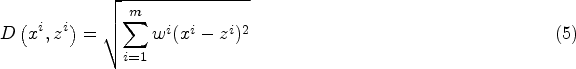
For practical implementation, $Δ_{outputs}$ is calculated as the maximum difference in prediction values when varying a feature across its range:

Δ_{outputs} = max_{i, j} | {outputs}_{i} - {outputs}_{j} |,

(6)

where

{outputs}_{i}

and

{outputs}_{j}

represent any two prediction values when varying the feature value. This approach captures the largest prediction change caused by the feature variation, providing a robust measure of feature sensitivity.

As shown in Figure 3, features with larger $Δ_{outputs}$ values (e.g., prothrombin time with 0.84) will receive more focused sampling around their critical values compared to features with smaller variations (e.g., gender with 0.038). This adaptive sampling strategy ensures that the explanation model captures the most influential feature relationships while maintaining comprehensive coverage of the feature space.

Figure 3.

$Δ_{outputs}$ of single feature sensitivity analysis. (a) Sex and (b) Protime.

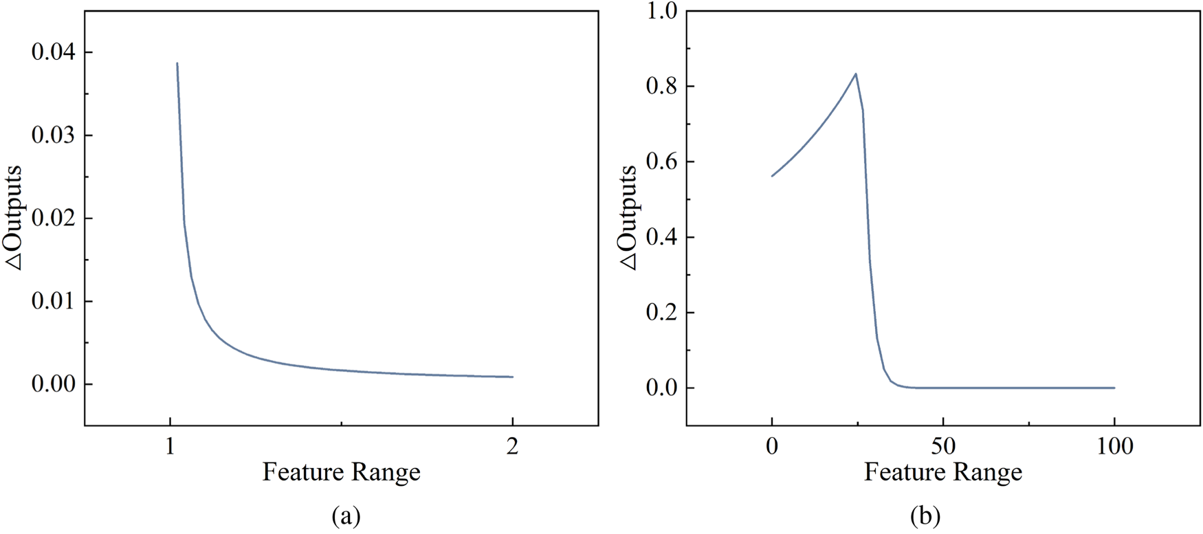
In summary, the weighted Euclidean distance allows different features to be weighted, thus considering feature importance, which can better reflect the degree of contribution of different features to the distance. This is especially important for features with different scales and importance, which can avoid the influence of some insensitive features on the distance calculation and is more in line with the idea of local model-agnostic linear regression methods.

3.2. Critical Value Range Determination and Sample Generation

After obtaining the feature sensitivity values, ELIME identifies critical value ranges where changes in feature values lead to significant shifts in model predictions. This approach helps to better capture the local decision boundary characteristics and generate more informative perturbation samples for subsequent linear regression fitting.

The critical value range for each feature is determined by analyzing how the model’s predictions change across different feature values:

critical_points = {i | Δ_{{outputs}_{i}} > threshold},

(7)

where

threshold

(default value 0.1) determines the significance of prediction changes. The

Δ_{{outputs}_{i}}

represents the difference between consecutive prediction values when varying the feature. If no critical points are found using the initial threshold, the algorithm adaptively adjusts to ensure at least some critical points are identified, falling back to the entire feature range only as a last resort.

For sample generation, ELIME employs a stratified approach based on these critical ranges. For continuous features, ELIME employs a dual sampling strategy: (1)

Sixty percent (60%) of samples are generated near the critical range using a normal distribution centered at the midpoint of the critical range with a standard deviation of 0.2 times the range width.

(2)

Forty percent (40%) of samples are uniformly distributed across the feature’s entire valid range.

For categorical features, the sampling maintains fixed proportions based on the identified critical values. When no critical values are found (i.e.,

Δ_{outputs} \leq threshold

), the algorithm falls back to sampling based on the feature’s observed frequency distribution in the test set.

These generated samples, combined with the weighted Euclidean distance metric, are then used in the same linear regression fitting process as LIME to create a locally interpretable model. The key difference lies in how ELIME generates these samples, using feature sensitivity analysis and critical value-based sampling to produce more representative perturbations. This approach leads to more accurate and reliable local explanations while maintaining the computational efficiency of LIME’s linear regression framework.

4. Experimental Setup and Evaluation

To comprehensively evaluate ELIME’s performance alongside LIME, DLIME, and AL-DLIME, we conduct experiments using established evaluation metrics from recent interpretability research. Our evaluation framework combines and adapts metrics from several key studies in the field. The experimental equipment’s CPU is an Intel i5-9300HF, 2.40 GHz, and the graphics card is an NVIDIA GeForce GTX1650 with 4 GB of video memory.

4.1. Experimental Setup

Datasets. We use two healthcare domain datasets from the UCI repository. The Hepatitis Patient (HP) dataset (Diaconis & Efron, 1983) contains 155 instances with 19 features, including demographic information (age, sex), clinical symptoms, and laboratory test results. The target variable is binary, indicating patient survival status (DIE/LIVE). The Indian Liver Patient Dataset (ILPD; Ramana et al., 2011) consists of 583 instances with 10 features, comprising demographic data and blood test results. The target variable indicates the presence (1) or absence (0) of liver disease. After standardization and preprocessing, both datasets are split into training and test sets with a ratio of $4 : 1$ .

Black Model Setting. Due to the small size of the dataset, we chose to use a decision tree classifier as the black-box model. This not only helps to handle the limited amount of data but also allows for consistency with existing methods (such as AL-DLIME) for effective comparison. The decision tree is configured with Gini impurity, setting the minimum number of samples per leaf to 1, the minimum number of samples for a split to 2, and the maximum number of features to the square root of the total number of features. The trained model achieves accuracies of 100% and 68.74% on the HP dataset and ILPD, respectively, providing a suitable foundation for our interpretation experiments.

Interpretation Methods. For LIME, we generate 5,000 perturbed samples per instance to ensure robust local explanations. DLIME and AL-DLIME utilize hierarchical clustering to prepare clustered data from the test sets, ensuring consistent feature selection. ELIME employs single-feature analysis with the test sets.

4.2. Evaluation Metrics

The evaluation of interpretation methods requires comprehensive metrics to assess their reliability and effectiveness. Following the evaluation framework established by Ribeiro et al. (2016) and extended by subsequent studies, we adopt three key metrics: stability, fidelity, and accuracy, each measuring different aspects of interpretation quality.

4.2.1. Stability

Zafar and Khan (2021) used Jaccard’s distance for evaluating interpretation consistency, and measures how reliably an interpretation method produces similar explanations for the same instance across multiple runs. For each instance, we generate 10 explanations and compute the pairwise Jaccard similarity (Kosub, 2019) coefficient between feature sets identified in different runs. For two feature sets $e_{i}$ and $e_{j}$ from different runs, the Jaccard similarity is calculated as:

J (e_{i}, e_{j}) = \frac{| e_{i} \cap e_{j} |}{| e_{i} \cup e_{j} |} .

(8)

The final stability score for an instance is computed by averaging the pairwise similarities across all 10 runs, with higher values indicating more stable explanations. This metric, widely used in interpretation evaluation studies (Molnar, 2020), provides a robust measure of interpretation consistency.

A stability score closer to 1.0 indicates higher consistency in feature identification across multiple runs, which is desirable as it demonstrates the method’s reliability in producing consistent interpretations.

4.2.2. Fidelity

LIME extracts a set of “golden features” from the black-box model and compares this feature set with the features identified by the interpretable model to evaluate fidelity. DLIME uses the cosine similarity between true predictions and the predictions from the interpretable model to quantitatively assess the fidelity of the explanation results. We propose a more direct evaluation approach inspired by LIME’s fidelity assessment method. Similarly, our fidelity metric leverages the interpretable nature of decision trees by directly comparing the features identified by our interpretation method with those actually used in the decision tree’s path. For an instance $x$ , we first obtain the set of features $F_{path} (x)$ used in the decision tree’s path, then generate an interpretation with the same number of features $F_{interp} (x)$ . The fidelity score is calculated as:

Fidelity (x) = \frac{| F_{interp} (x) \cap F_{path} (x) |}{| F_{interp} (x) \cup F_{path} (x) |} .

(9)

This adaptation provides a more direct measure of interpretation quality by evaluating how accurately the method identifies the truly important features used in the model’s decision-making process.

Higher fidelity scores (closer to 1.0) indicate better alignment between the interpretation method’s identified features and the actual features used in the decision tree’s decision path, demonstrating more accurate feature importance identification.

4.2.3. Accuracy

For accuracy assessment, we implement two complementary feature deletion experiments, building upon the methodology proposed by Hooker et al. (2019) and Ancona et al. (2018). This dual-approach evaluation provides a more comprehensive understanding of feature importance:

(1)
Single feature deletion evaluates the impact of removing pairs of the most important features in each round. For a given instance x and its important feature pairs $F_{p}$ , the accuracy score is computed as:
${Accuracy}_{single} (x) = 1 - \frac{1}{| F_{p} |} \sum_{(f_{1}, f_{2}) \in F_{p}} | P (x) - P (x_{- (f_{1}, f_{2})}) |,$
(10)
where $P (x)$ is the original prediction probability, and $P (x_{- (f_{1}, f_{2})})$ is the prediction probability after modifying the feature pair $(f_{1}, f_{2})$ .
(2)
Incremental feature deletion progressively masks features in order of their importance, measuring the cumulative impact on predictions. For an instance x and its ordered feature set $F = {f_{1}, \dots, f_{n}}$ , the accuracy is calculated as:
${Accuracy}_{incremental} (x, k) = 1 - | P (x) - P (x_{- {f_{1}, \dots, f_{k}}}) |,$
(11)
where $k$ represents the number of features masked in each round. For both experiments, we implement feature modification by replacing feature values with their opposite values from the training data distribution: for categorical features (such as sex and presence of symptoms), we use the alternative category, while for continuous features (such as bilirubin levels), we select values from the opposite end of the distribution—using the 10th percentile value if the original value is above the 75th percentile, and vice versa. This approach maintains the data’s structural integrity while effectively neutralizing the feature’s original impact.
Both deletion experiments are conducted over multiple rounds $(n = 5)$ and averaged across different test instances to ensure robust evaluation. In these experiments, lower scores indicate that the modified features have a greater impact on the model’s predictions, suggesting better feature importance identification. Particularly, lower scores in the early rounds (especially round 1) are especially significant, as they indicate that the interpretation method successfully identified the most crucial features first. This is because: (1)
In single feature deletion, a low initial score means the first pair of identified features significantly affects the model’s predictions when modified.
(2)
In incremental deletion, a low initial score indicates that the first features identified are indeed the most influential, as their modification causes the largest deviation from the original predictions.
This comprehensive accuracy evaluation framework allows us to validate both the individual and cumulative importance of features identified by our interpretation method. The early-round performance is particularly important as it demonstrates the method’s ability to prioritize the most influential features, while the overall pattern across rounds provides insights into the method’s feature importance ranking capability.
5. Experimental Results

Figure 4 demonstrates the interpretation results from different methods on the same instance from the HP dataset. For each method, we present two separate interpretation runs (top and bottom rows) to illustrate the consistency of feature importance identification across multiple explanations of the same instance.

Figure 4.

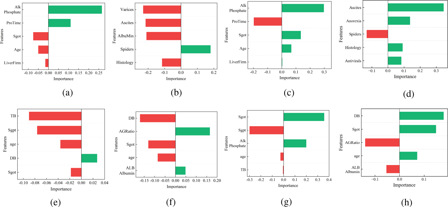
Interpretation results of different interpretation methods for HP instances: (a) LIME, (b) DLIME, (c) ELIME, (d) AL-DLIME, (e) LIME, (f) DLIME, (g) ELIME, and (h) AL-DLIME. Note. LIME = local interpretable model-agnostic explanation; DLIME = deterministic LIME; ELIME = exact LIME; AL-DLIME = active learning-based DLIME.

The interpretation results are visualized as bar charts, where the length and color of each bar represent both the magnitude and direction of feature importance. Green bars indicate a positive correlation with the prediction (supporting features), while red bars show a negative correlation (opposing features). The absolute length of each bar corresponds to the feature’s importance weight in the interpretation.

Comparing the two runs for each method reveals different levels of consistency. LIME shows notable variations between runs, with features such as “Phosphate” and “ProTime” changing in both importance and direction. DLIME and AL-DLIME demonstrate high consistency, maintaining the same feature sets and importance rankings across runs. ELIME shows improved stability over LIME while preserving some natural variation in feature importance weights. These initial visual comparisons motivate our subsequent quantitative analysis, where we will systematically evaluate each method’s performance through three key metrics: stability, fidelity, and accuracy. The following sections present detailed experimental results that validate these preliminary observations and provide comprehensive insights into the relative strengths of each interpretation approach.

5.1. Stability

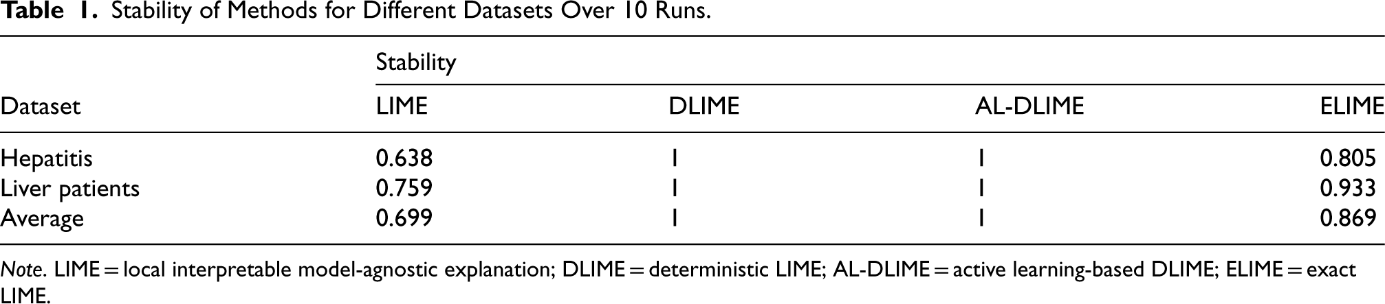
Table 1 presents the stability comparison among LIME, DLIME, AL-DLIME, and ELIME methods across different datasets. The experimental results show that DLIME and AL-DLIME achieve perfect stability (1.0) for all datasets. This is due to two main reasons: first, although the feature importance values may vary between runs, the ranking of features remains consistent. Our stability evaluation focuses on feature ranking consistency, which results in a perfect score when the order is unchanged. Second, both DLIME and AL-DLIME employ deterministic mechanisms in their sampling and feature selection processes, ensuring consistent feature rankings across multiple runs.

Table 1.
Stability of Methods for Different Datasets Over 10 Runs.

$Stability$

Dataset LIME DLIME AL-DLIME ELIME

Hepatitis 0.638 1 1 0.805

Liver patients 0.759 1 1 0.933

Average 0.699 1 1 0.869

	$Stability$
Hepatitis	0.638	1	1	0.805
Liver patients	0.759	1	1	0.933
Average	0.699	1	1	0.869

Note. LIME = local interpretable model-agnostic explanation; DLIME = deterministic LIME; AL-DLIME = active learning-based DLIME; ELIME = exact LIME.

In contrast, ELIME shows improved stability over LIME, with average stability scores of 0.805 and 0.933 for the hepatitis and liver patients datasets, respectively. This improvement is attributed to ELIME’s use of single-feature analysis, which enhances the consistency of feature selection. However, ELIME still allows for some variability in feature importance values, which is why its stability is not as high as DLIME and AL-DLIME.

Figure 5 visualizes the stability performance of each method on the HP dataset. LIME exhibits the lowest stability, with significant variations in feature rankings between runs. DLIME and AL-DLIME maintain consistent feature rankings, as indicated by the uniform patterns in their heatmaps. ELIME, while not achieving perfect stability, demonstrates a more stable feature selection process compared to LIME, highlighting its balanced approach to interpretation.

Figure 5.

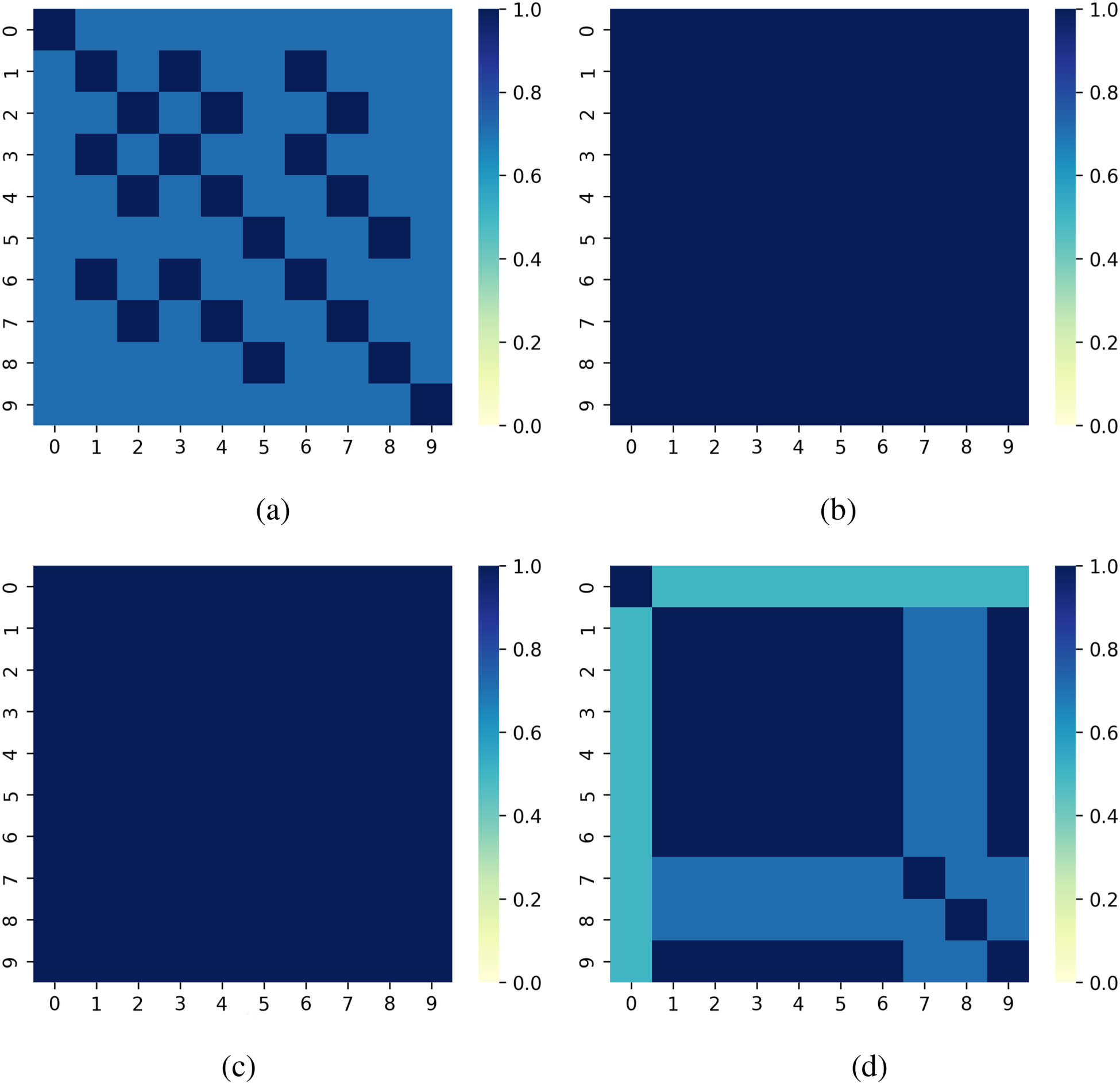
Comparison of different methods’ stability on different instances for Hepatitis Patient dataset: (a) LIME, (b) DLIME, (c) AL-DLIME, and (d) ELIME. Note. LIME = local interpretable model-agnostic explanation; DLIME = deterministic LIME; AL-DLIME = active learning-based DLIME; ELIME = exact LIME.

These results suggest that while DLIME and AL-DLIME achieve perfect stability through deterministic approaches, ELIME provides a more flexible solution by maintaining high stability while allowing for necessary variability in feature importance.

5.2. Fidelity

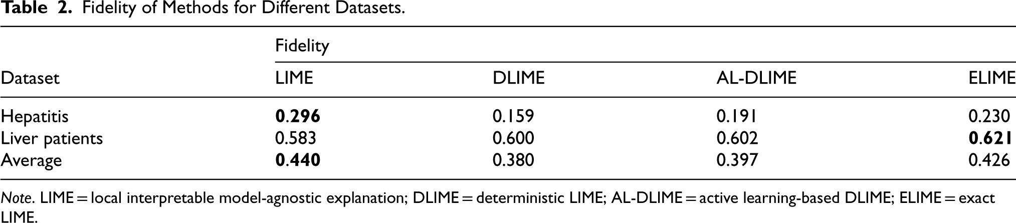
Table 2 presents the fidelity comparison among LIME, DLIME, AL-DLIME, and ELIME methods across different datasets. The experimental results show that ELIME achieves the highest average fidelity (average 0.426) compared to DLIME and AL-DLIME (average 0.380 and 0.397). This superior performance can be attributed to ELIME’s single-feature analysis approach, which allows it to more accurately identify the truly important features used in the decision tree’s path. In the table, bold values denote the highest fidelity scores per dataset, highlighting the top-performing method.

The fidelity performance varies significantly between datasets, primarily due to their different sizes. For the Hepatitis dataset (155 instances), all methods show relatively low fidelity scores (0.159–0.296), with LIME achieving marginally better performance (0.296) than ELIME (0.230). This suggests that with limited data, all methods struggle to accurately identify the decision tree’s key features, though LIME maintains a slight advantage.

In contrast, for the larger Liver Patient dataset (583 instances), all methods show improved fidelity scores (0.583–0.621). DLIME, AL-DLIME, and ELIME achieve similar performance, while LIME shows slightly lower fidelity (0.583). This improvement across all methods with larger data volume indicates that more data helps methods better capture the model’s decision-making process. However, ELIME still maintains its advantage, suggesting that its feature analysis approach is more robust across different data conditions.

These results demonstrate that while data size significantly impacts fidelity performance, ELIME’s approach to feature importance analysis provides reliable interpretations regardless of dataset size.

5.3. Accuracy

Tables 3 through 6 present the results of feature importance evaluation through deletion experiments on both HP dataset and ILPD. The values represent the similarity between the model’s original predictions and predictions after feature deletion, where lower values indicate a greater impact of deleted features, thus suggesting better feature importance identification. In these tables, the lowest first-round similarity scores are highlighted in bold, indicating that the corresponding method was most effective at identifying crucial features from the outset.

Table 2.
Fidelity of Methods for Different Datasets.

$Fidelity$

Dataset LIME DLIME AL-DLIME ELIME

Hepatitis 0.296 0.159 0.191 0.230

Liver patients 0.583 0.600 0.602 0.621

Average 0.440 0.380 0.397 0.426

	$Fidelity$
Hepatitis	0.296	0.159	0.191	0.230
Liver patients	0.583	0.600	0.602	0.621
Average	0.440	0.380	0.397	0.426

Note. LIME = local interpretable model-agnostic explanation; DLIME = deterministic LIME; AL-DLIME = active learning-based DLIME; ELIME = exact LIME.

Table 3.

Results for Single Feature Deletion Across Five Rounds (HP Datasets).

	Round
Model	1	2	3	4	5
LIME	0.667	0.933	1.000	1.000	1.000
DLIME	0.933	0.867	0.800	0.867	1.000
AL-DLIME	0.867	0.800	0.933	0.933	0.867
ELIME	0.533	0.667	0.867	0.933	1.000

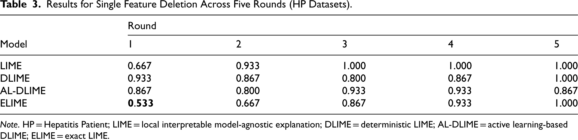
Note. HP = Hepatitis Patient; LIME = local interpretable model-agnostic explanation; DLIME = deterministic LIME; AL-DLIME = active learning-based DLIME; ELIME = exact LIME.

For single feature deletion on the smaller HP dataset (Table 3), ELIME demonstrates superior performance with the lowest first-round similarity score (0.533), significantly outperforming LIME (0.667), AL-DLIME (0.867), and DLIME (0.933). This indicates ELIME’s strong capability in identifying important feature pairs when working with limited data.

The subsequent rounds reveal distinct patterns for different methods. Theoretically, as less important features are modified in later rounds, the similarity scores should increase, eventually approaching 1.000 when truly unimportant features are being modified. ELIME follows this expected pattern with gradually increasing scores (0.533–1.000), suggesting it correctly identifies and ranks features based on their true importance. LIME also shows an increasing trend and reaches perfect similarity (1.000) quickly by round 3.

In contrast, AL-DLIME shows concerning fluctuations, with scores actually decreasing in later rounds (0.933–0.867). This unexpected pattern suggests that with limited data, AL-DLIME may have incorrectly pushed some important features to later rounds in its ranking. Similarly, DLIME’s nonmonotonic pattern (0.867–0.800–0.867) indicates potential issues in feature importance ordering when working with small datasets.

The HP incremental deletion experiment (Table 4) reveals more complex patterns in feature importance identification. While ELIME achieves the lowest first-round similarity (0.600), its subsequent performance shows unexpected fluctuations (0.667–0.533 and back to 0.600). DLIME and AL-DLIME show a more expected pattern with steadily decreasing scores from high initial values (1.000 and 0.933) to lower levels (0.733). However, LIME’s erratic pattern (0.733–0.800–0.600) suggests potential issues with contrasting features, similar to what we observed in the ILPD later.

Table 4.

Results for Incremental Feature Deletion Across Five Rounds (HP Datasets).

	Round
Model	1	2	3	4	5
LIME	0.733	0.733	0.800	0.667	0.600
DLIME	1.000	0.933	0.800	0.800	0.733
AL-DLIME	0.933	0.867	0.800	0.733	0.733
ELIME	0.600	0.667	0.533	0.533	0.600

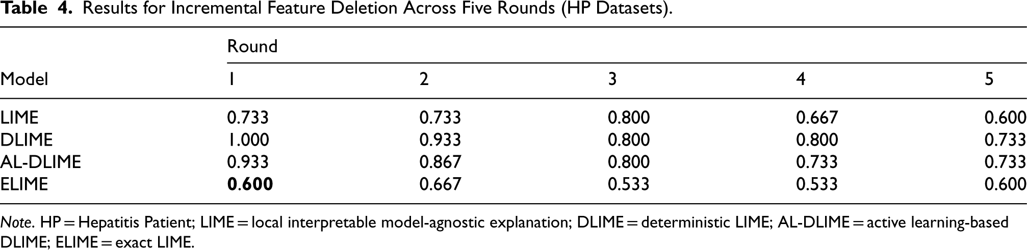
Note. HP = Hepatitis Patient; LIME = local interpretable model-agnostic explanation; DLIME = deterministic LIME; AL-DLIME = active learning-based DLIME; ELIME = exact LIME.

These results, when combined with the single deletion findings, reveal an interesting dynamic in small datasets: the complex interplay between positively influential features and contrasting features becomes more pronounced when working with limited data, making it harder for all methods to consistently rank feature importance, though each shows different strengths in different evaluation contexts.

Interestingly, when tested on the larger ILPD, the results reveal different patterns. In single feature deletion (Table 5), while DLIME and LIME achieve better first-round scores (0.667) compared to ELIME and AL-DLIME (0.733), the subsequent rounds tell a more complex story. LIME’s fluctuating pattern (0.733, 0.667, 0.800, 0.667) is particularly revealing—these oscillations suggest that LIME has incorrectly prioritized multiple contrasting features (features that push predictions in the opposite direction) in its importance ranking. When these contrasting features are removed, the model’s predictions actually become more similar to the original predictions, resulting in higher similarity scores.

Table 5.

Results for Single Feature Deletion Across Five Rounds (ILPD Datasets).

	Round
Model	1	2	3	4	5
LIME	0.667	0.733	0.667	0.800	0.667
DLIME	0.667	0.667	0.667	0.667	0.867
AL-DLIME	0.733	0.600	0.600	0.533	0.933
ELIME	0.733	0.667	0.600	0.733	0.933

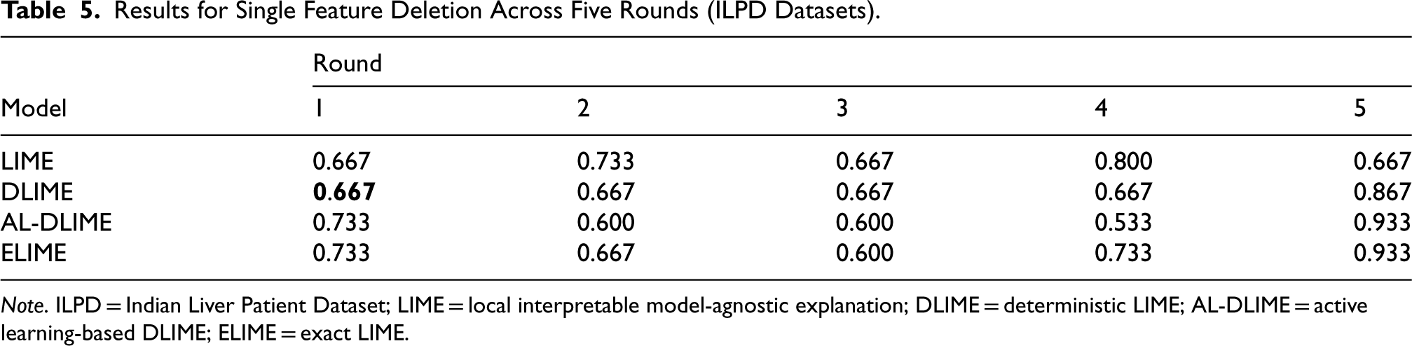
Note. ILPD = Indian Liver Patient Dataset; LIME = local interpretable model-agnostic explanation; DLIME = deterministic LIME; AL-DLIME = active learning-based DLIME; ELIME = exact LIME.

Table 6.

Results for Incremental Feature Deletion Across Five Rounds (ILPD Datasets).

	Round
Model	1	2	3	4	5
LIME	0.867	0.733	0.800	0.733	0.600
DLIME	0.800	0.667	0.600	0.600	0.667
AL-DLIME	0.733	0.733	0.600	0.600	0.667
ELIME	0.667	0.733	0.533	0.533	0.533

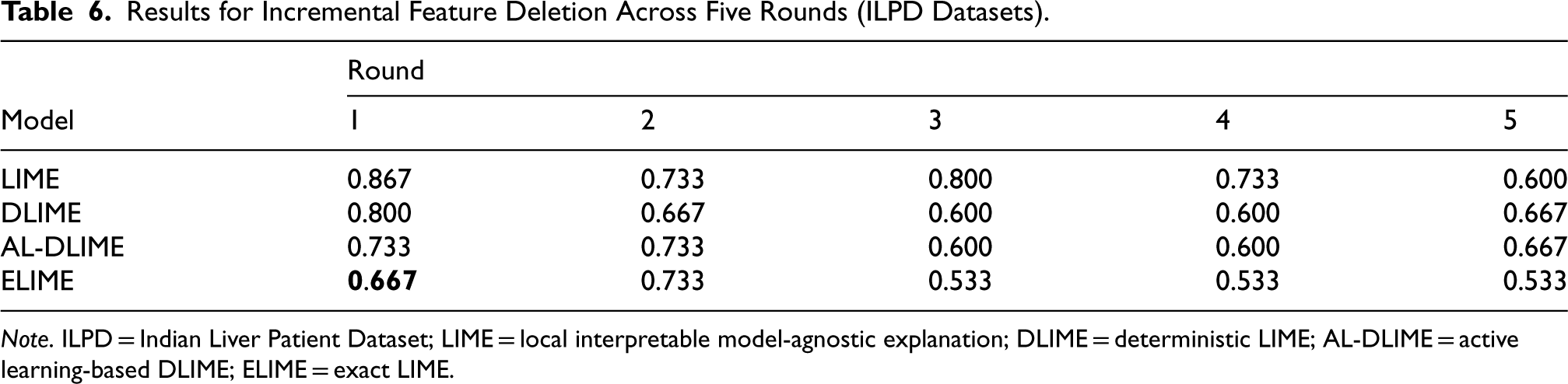
Note. ILPD = Indian Liver Patient Dataset; LIME = local interpretable model-agnostic explanation; DLIME = deterministic LIME; AL-DLIME = active learning-based DLIME; ELIME = exact LIME.

The other three methods demonstrate a more logical pattern: they show decreasing similarity scores until reaching a turning point, indicating they have correctly identified positively influential features first. Specifically, ELIME reaches its lowest point at round 3 (0.600), while DLIME maintains stability until round 4 and AL-DLIME continues decreasing until round 4 (0.533) before increasing. This systematic decrease followed by an increase suggests these methods first identify genuinely important features before encountering contrasting features in later rounds.

In the ILPD incremental deletion experiment (Table 6), ELIME achieves the lowest first-round similarity score (0.667), followed by AL-DLIME (0.733), DLIME (0.800), and LIME (0.867). The high initial score and subsequent fluctuations in LIME’s performance further confirm its tendency to misrank contrasting features. DLIME and AL-DLIME show a gradual decrease until round 3 (0.600) before stabilizing or slightly increasing, while ELIME reaches and maintains the lowest similarity score (0.533) from round 3 onwards, suggesting it most effectively identifies and orders truly influential features.

These findings reveal a crucial distinction in feature importance identification: while all methods can identify important features, ELIME and clustering-based methods (DLIME and AL-DLIME) are better at distinguishing between positively influential features and contrasting features. LIME’s performance suggests it may struggle with this distinction, often ranking contrasting features alongside or ahead of positively influential ones. This ability to properly order features based on their true directional impact is particularly important for real-world applications where understanding the nature of feature influence is crucial for decision-making.

6. Conclusions

This paper introduces ELIME, an enhanced model-agnostic interpretation method for tabular data that improves upon existing methods through single-feature analysis and deterministic sampling. Our comprehensive experiments reveal several key strengths of ELIME: (1) superior performance in identifying important feature pairs when working with limited data, (2) consistent ability to identify the most crucial individual features regardless of dataset size, and (3) better capability in distinguishing between positively influential features and contrasting features compared to LIME. These characteristics make ELIME particularly valuable for applications where precise feature importance identification is crucial, especially in scenarios with limited data availability. The key innovations of ELIME—single-feature analysis and deterministic sampling based on hierarchical clustering—not only contribute to more reliable and accurate interpretations, but also help maintain the model-agnostic nature of LIME while addressing its limitations in feature importance ranking.

Future work will focus on extending ELIME to handle more complex data types and exploring ways to further enhance the method’s ability to capture feature interactions, particularly in scenarios where contrasting features play significant roles in model predictions.

Footnotes

ORCID iDs

Junyan Qian

Xiaofu Du

Ming Ling

Hao Ding

Funding

The authors disclosed receipt of the following financial support for the research, authorship, and/or publication of this article: This work was supported by the Guangxi Natural Science Foundation of China under Grant 2024GXNSFBA010248, in part by the National Natural Science Foundation of China under Grants 62162004 and U21A20474, and in part by Guangxi Collaborative Innovation Center of Multi-Source Information Integration and Intelligent Processing.

Declaration of Conflicting Interests

The authors declared no potential conflicts of interest with respect to the research, authorship, and/or publication of this article.

References

Ancona

Ceolini

Öztireli

Gross

(2018). Towards better understanding of gradient-based attribution methods for deep neural networks. In Proceedings of the International conference on learning representations (ICLR) (pp. 1–16). OpenReview.net. https://openreview.net/forum?id=Sy21R9JAW

Diaconis

Efron

(1983). Computer-intensive methods in statistics. Scientific American, 248, 116–131. https://www.jstor.org/stable/24968902

Dwivedi

Dave

Naik

Singhal

Omer

Patel

Qian

Wen

Shah

Morgan

, et al. (2023). Explainable AI (XAI): Core ideas, techniques, and solutions. ACM Computing Surveys, 55, 1–33. https://doi.org/10.1145/3561048

Hassija

Chamola

Mahapatra

Singal

Goel

Huang

Scardapane

Spinelli

Mahmud

Hussain

(2024). Interpreting black-box models: A review on explainable artificial intelligence. Cognitive Computation, 16, 45–74. https://doi.org/10.1007/s12559-023-10179-8

Henckaerts

Antonio

Côté

M.-P.

(2022). When stakes are high: Balancing accuracy and transparency with model-agnostic interpretable data-driven surrogates. Expert Systems with Applications, 202, 117230. https://doi.org/10.1016/j.eswa.2022.117230

Holm

Macedo

(2023). The accuracy and faithfullness of AL-DLIME-active learning-based deterministic local interpretable model-agnostic explanations: A comparison with LIME and DLIME in medicine. In L. Longo (Ed.) Explainable artificial intelligence (vol. 1901, pp. 33–99). Springer. https://doi.org/10.1007/978-3-031-44064-9_31

Hooker

Erhan

Kindermans

P.-J.

Kim

(2019). A benchmark for interpretability methods in deep neural networks. In Proceedings of the International conference on neural information processing systems (NeurIPS) (pp. 1–12). Curran Associates. https://proceedings.neurips.cc/paper_files/paper/2019/file/fe4b8556000d0f0cae99daa5c5c5a410-Paper.pdf

Julian

K. D.

Kochenderfer

M. J.

Owen

M. P.

(2019). Deep neural network compression for aircraft collision avoidance systems. Journal of Guidance, Control, and Dynamics, 42, 598–608. https://doi.org/10.2514/1.G003724

Katuwal

G. J.

Chen

(2016). Machine learning model interpretability for precision medicine. 1–4. arXiv preprint arXiv:1610.09045.

10.

Kaur

Uslu

Durresi

Badve

Dundar

(2021). Trustworthy explainability acceptance: A new metric to measure the trustworthiness of interpretable AI medical diagnostic systems. In Complex, intelligent and software intensive systems: Proceedings of the 15th international conference on complex, intelligent and software intensive systems (CISIS-2021) (vol. 278, pp. 35–46). Springer. https://doi.org/10.1007/978-3-030-79725-6_4

11.

Kaur

Uslu

Rittichier

K. J.

Durresi

(2022). Trustworthy artificial intelligence: a review. ACM Computing Surveys (CSUR), 55, 1–38. https://doi.org/10.1145/3491209

12.

Kermany

D. S.

Goldbaum

Cai

Valentim

C. C.

Liang

Baxter

S. L.

McKeown

Yang

Yan

, et al. (2018). Identifying medical diagnoses and treatable diseases by image-based deep learning. Cell, 172, 1122–1131. https://www.cell.com/cell/fulltext/S0092-8674(18)30154-5

13.

Kosub

(2019). A note on the triangle inequality for the Jaccard distance. Pattern Recognition Letters, 120, 36–38. https://doi.org/10.1016/j.patrec.2018.12.007

14.

Rezaeipanah

El Din

E. M. T.

(2022). An ensemble agglomerative hierarchical clustering algorithm based on clusters clustering technique and the novel similarity measurement. Journal of King Saud University-Computer and Information Sciences, 34, 3828–3842. https://doi.org/10.1016/j.jksuci.2022.04.010

15.

Longo

Brcic

Cabitza

Choi

Confalonieri

Del Ser

Guidotti

Hayashi

Herrera

Holzinger

, et al. (2024). Explainable artificial intelligence (XAI) 2.0: A manifesto of open challenges and interdisciplinary research directions. Information Fusion, 106, 102301. https://doi.org/10.1016/j.inffus.2024.102301

16.

Lundberg

S. M.

Lee

S.-I.

(2017). A unified approach to interpreting model predictions. Advances in Neural Information Processing Systems, 4768–4777. https://dl.acm.org/doi/abs/10.5555/3295222.3295230

17.

Manfredi

Jestin

(2016). An introduction to ACAS Xu and the challenges ahead. In 2016 IEEE/AIAA 35th digital avionics systems conference (DASC) (pp. 1–9). IEEE. https://doi.org/10.1109/DASC.2016.7778055

18.

Mersha

Lam

Wood

AlShami

Kalita

(2024). Explainable artificial intelligence: A survey of needs, techniques, applications, and future direction. Neurocomputing, 599, 128111. https://doi.org/10.1016/j.neucom.2024.128111

19.

Minh

Wang

H. X.

Y. F.

Nguyen

T. N.

(2022). Explainable artificial intelligence: a comprehensive review. Artificial Intelligence Review, 55, 3503–3568. https://doi.org/10.1007/s10462-021-10088-y

20.

Molnar

(2020). Interpretable machine learning: A guide for making black box models explainable (pp. 140–235). Leanpub.

21.

Moreira

Sindhgatta

Ouyang

Bruza

Wichert

(2020). An investigation of interpretability techniques for deep learning in predictive process analytics. 1–15. arXiv preprint arXiv:2002.09192.

22.

Morooka

F. E.

Junior

A. M.

Sigahi

T. F.

Pinto

J. D. S.

Rampasso

I. S.

Anholon

(2023). Deep learning and autonomous vehicles: Strategic themes, applications, and research agenda using SciMAT and content-centric analysis, a systematic review. Machine Learning and Knowledge Extraction, 5, 763–781. https://doi.org/10.3390/make5030041

23.

Nguyen

T.-D.

Cherif

Mahieux

P.-Y.

Lux

Aït-Mokhtar

Bastidas-Arteaga

(2023). Artificial intelligence algorithms for prediction and sensitivity analysis of mechanical properties of recycled aggregate concrete: A review. Journal of Building Engineering, 66, 105929. https://doi.org/10.1016/j.jobe.2023.105929

24.

Ramana

B. V.

Babu

M. S. P.

Venkateswarlu

, et al. (2011). A critical study of selected classification algorithms for liver disease diagnosis. International Journal of Database Management Systems, 3, 101–114. https://doi.org/10.5121/ijdms.2011.3207

25.

Ribeiro

M. T.

Singh

Guestrin

(2016). “Why should I trust you?” explaining the predictions of any classifier. In Proceedings of the 22nd ACM SIGKDD international conference on knowledge discovery and data mining (pp. 1135–1144). ACM. https://doi.org/10.1145/2939672.2939778

26.

Selvaraju

R. R.

Cogswell

Das

Vedantam

Parikh

Batra

(2020). Grad-cam: Visual explanations from deep networks via gradient-based localization. In Proceedings of the IEEE International Conference on Computer Vision (ICCV) (pp. 618–626). IEEE. https://doi.org/10.1007/s11263-019-01228-7

27.

Shinde

(2023). Deep learning approaches for medical image analysis and disease diagnosis. International Journal of Multidisciplinary Innovation and Research Methodology, 2, 57–66. https://doi.org/10.1155/2021/6215281

28.

Van der Velden

B. H.

Kuijf

H. J.

Gilhuijs

K. G.

Viergever

M. A.

(2022). Explainable artificial intelligence (XAI) in deep learning-based medical image analysis. Medical Image Analysis, 79, 102470. https://doi.org/10.1016/j.media.2022.102470

29.

Yang

Xia

(2022). Unbox the black-box for the medical explainable AI via multi-modal and multi-centre data fusion: A mini-review, two showcases and beyond. Information Fusion, 77, 29–52. https://doi.org/10.1016/j.inffus.2021.07.016

30.

Zafar

M. R.

Khan

(2021). Deterministic local interpretable model-agnostic explanations for stable explainability. Explainable Artificial Intelligence (XAI), 3, 525–541. https://doi.org/10.3390/make3030027

31.

Zhang

A. Y.

Lam

S. S. W.

Liu

Pang

Chan

L. L.

Tang

P. H.

(2018). Development of a radiology decision support system for the classification of MRI brain scans. In Proceedings of the 2018 IEEE/ACM 5th international conference on big data computing applications and technologies (BDCAT) (pp. 107–115). IEEE. https://doi.org/10.1109/BDCAT.2018.00021

32.

Zhou

Khosla

Lapedriza

Oliva

Torralba

(2016). Learning deep features for discriminative localization. In Proceedings of the IEEE conference on computer vision and pattern recognition (CVPR) (pp. 2921–2929). IEEE. https://doi.org/10.1109/CVPR.2016.319

	$Stability$
Dataset	LIME	DLIME	AL-DLIME	ELIME
Hepatitis	0.638	1	1	0.805
Liver patients	0.759	1	1	0.933
Average	0.699	1	1	0.869

ELIME: Exact Local Interpretable Model-Agnostic Explanation

Abstract

Keywords

1. Introduction

2.1. Model-Related Explanation Methods

2.2. Model-Agnostic Explanation Methods

3. ELIME Framework

4.1. Experimental Setup

4.2. Evaluation Metrics

4.2.1. Stability

Table 1. Stability of Methods for Different Datasets Over 10 Runs. Stability Dataset LIME DLIME AL-DLIME ELIME Hepatitis 0.638 1 1 0.805 Liver patients 0.759 1 1 0.933 Average 0.699 1 1 0.869

5.3. Accuracy

Table 2. Fidelity of Methods for Different Datasets. Fidelity Dataset LIME DLIME AL-DLIME ELIME Hepatitis 0.296 0.159 0.191 0.230 Liver patients 0.583 0.600 0.602 0.621 Average 0.440 0.380 0.397 0.426

Footnotes

ORCID iDs

Funding

Declaration of Conflicting Interests

References

Table 1.
Stability of Methods for Different Datasets Over 10 Runs.

$Stability$

Dataset LIME DLIME AL-DLIME ELIME

Hepatitis 0.638 1 1 0.805

Liver patients 0.759 1 1 0.933

Average 0.699 1 1 0.869

Table 2.
Fidelity of Methods for Different Datasets.

$Fidelity$

Dataset LIME DLIME AL-DLIME ELIME

Hepatitis 0.296 0.159 0.191 0.230

Liver patients 0.583 0.600 0.602 0.621

Average 0.440 0.380 0.397 0.426