SCOP: Schrödinger Control Optimal Planning for Goal-based Wealth Management

Abstract

We consider the problem of optimization of contributions of a financial planner such as a working individual towards a financial goal such as retirement. The objective of the planner is to find an optimal and feasible schedule of periodic installments to an investment portfolio set up towards the goal. Because portfolio returns are random, the practical version of the problem amounts to finding an optimal contribution scheme such that the goal is satisfied at a given confidence level. This paper suggests a semi-analytical approach to a continuous-time version of this problem based on a controlled backward Kolmogorov equation (BKE) which describes the tail probability of the terminal wealth given a contribution policy. The controlled BKE is solved semi-analytically by reducing it to a controlled Schrödinger equation and solving the latter using an algebraic method. Numerically, our approach amounts to finding semi-analytical solutions simultaneously for all values of control parameters on a small grid, and then using the standard two-dimensional spline interpolation to simultaneously represent all satisficing solutions of the original plan optimization problem. Rather than being a point in the space of control variables, satisficing solutions form continuous contour lines (efficient frontiers) in this space.

1. Introduction

We consider the problem of optimization of contributions of a financial planner such as a working individual towards a financial goal such as retirement. The objective of the planner is to find an optimal and feasible schedule of periodic installments to an investment portfolio set up towards the goal. Because portfolio returns are random, in practice this problem amounts to finding an optimal contribution scheme such that the goal is satisfied at a given confidence level. This problem is similar to the celebrated Merton (1971) optimal consumption problem (Merton, 1971), however it differs from the latter in at least three important aspects.

First, we do not address a portfolio optimization part of this problem, instead assuming that an investment portfolio set towards the goal has a fixed equity to cash ratio which is maintained by a financial fiduciary. This implies that a part of a regular cash contribution to the portfolio from the planner that is invested in equity is fixed by the fiduciary and is not subject to optimization. ¹

Second, we do not maximize any utility of consumption, and respectively do not consider any consumption process either. Instead, we work directly with contributions to the financial plan as decision variables constrained by a net income, and our objective is to exceed a certain target wealth level at a terminal time T at a given confidence level α. In this sense, our problem formulation fits the setting of goal-based wealth management, see e.g., Das et al. (2018) and references therein.

The problem as formulated belongs in the class of optimal stochastic control problems, and thus could in principle be solved using conventional tools such as dynamic programming (DP) or reinforcement learning (RL). ² However, our problem is not necessarily a problem of adaptive (closed-loop) control type that are usually addressed with DP and RL methods. Retirement planning usually involves setting up a plan upfront, which is then revisited, if necessary, on the annual basis. A typical plan usually involves a time line of annual installments, where annual contributions planned for the future are scheduled to increase to adjust for inflation, as well as possibly incorporate benefits from expected future increases in wages or other investable income. Such settings are typical for open-loop control problems, where an agent decides on the policy at the start, and then keeps it fixed for a certain fixed number of steps, without adapting it at each steps as is done in DP or RL.

Another important difference of our problem from the setting of DP or RL is that the latter methods solve a maximization problem for a value (or action-value) function. If the value function has a global maximum as a function of a deterministic policy, then there should be a policy - a point in a multi-dimensional action space whose position depends on the state - that attains this maximum. In contrast, a proper framework for decision-making in our setting is the framework of satisficing decision making of Simon (1955, 1979). With this framework, we do not maximize an objective function. Instead, we only want to bring it to a certain goal level that we define beforehand. This involves two steps: search (i.e., exploring the objective function for different values of input controls), and satisficing (i.e., picking a solution that satisfies the goal criterion) (Simon, 1979). Clearly, with this setting, feasible problems should in general produce continuous lines in the action space, rather than isolated points, as optimal solutions.

This paper suggests a semi-analytical solution to a continuous-time version of the problem formulated above. We use a probabilistic approach that amounts to analysis of two related equations. The first one is Fokker-Planck equation (FPE) whose solution is the probability density of the terminal wealth at the at time T, for a given contribution plan. The second equation is the backward Kolmogorov equation (BKE) which gives the probability of the terminal wealth to fall below a certain target wealth at a given confidence level α. We solve the resulting controlled FPE and BKE equations semi-analytically by reducing them to controlled Schrödinger equations, ³ and then solving the latter equations in a semi-closed form using an algebraic method. These semi-analytical solutions are computed simultaneously for all values of two control parameters describing annual contributions and their growth rate, on a small 2D grid of their discretized admissible values. Once the values of the tail BKE probability are computed for all nodes on the grid, its values for arbitrary inputs are cheaply obtained using the standard 2D cubic spline interpolation. This completes the search step of satisficing decision-making in our problem.

Once the search stage is completed, the satisficing part is rather simple, as all it takes is to draw constant-probability lines at the confidence levels α on the surface of the BKE tail probability function viewed as a function of initial controls. This task can be done using the standard 2D spline interpolation plus a root-finding algorithm, or equivalently using a contour-plotting algorithm that already combines the first two algorithms.

Therefore, in our approach, dubbed the Schrödinger Control Optimal Planning, or SCOP for short, the initial problem of contribution optimization amounts to the standard 2D spline interpolation plus a root-solving (or equivalently contour-plotting) algorithm, whose end result gives a visual representation of all possible satisficing plans at different confidence levels. Such visual representation is conceptualized via the notion of efficient frontiers: constant-level lines on the 2D surface of the BKE probability as the function of controls. This gives the planner the ability to perform a real time policy optimization for a given goal, or scenario analyses for different settings of the planning problem.

The paper is organized as follows. In Section 2, we present the theoretical framework for our problems. Section 3 describes our method for retirement plan optimization. Finally, a summary and an outlook for future research are presented in Section 4. All technical details and derivations are left to Appendices A, B, and C. The appendices have a hierarchical structure, i.e., Appendices B and C clarify certain technical details for topics discussed in Appendix A.

2. Optimal Contribution Problem

2.1. The Investment Portfolio Dynamics

We consider a financial planner such as a retirement planner with a planning horizon T who invests in a portfolio created towards a goal, expressed as a desired terminal wealth at time T. The investment portfolio has a fixed ratio 0 ≤ ω ≤ 1 of equity to the total portfolio value (e.g., ω = .9), which is assumed to be maintained by a fiduciary that manages the portfolio on client’s behalf.

Let c _t Δt be the after-tax money flow from the planner to the portfolio in the time step [t, t + Δt]. This investment of cash from the planner forces the fiduciary to buy the amount of equity equal to ωc _t Δt, which also incurs proportional transaction cost νω|c _t |Δt, where 0 ≤ ν ≤ 1 is a parameter. As we have c _t ≥ 0 in our problem, in what follows we omit the absolute value expression in the transaction cost formula.

The investment portfolio is composed of cash b _t and equity s _t . We assume that the cash infusion to the portfolio happens at time t₊ immediately after t, followed by an immediate purchase of equity by the fiduciary. The cash and equity positions at time t₊ are then obtained as follows:

$\begin{array}{lll}{b}_t^{+}& =& b_t+\left(\left(1-\omega \right)c_t-\nu \omega c_t\right)\mathrm{\Delta }t\\ s_t^{+}& =& s_t+\omega c_t\mathrm{\Delta }t\end{array}$

(1)

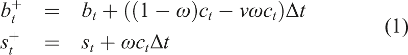
This produces the following update rule for the total portfolio value Π _t ≔ b _t + s _t :

${\mathrm{\Pi }}_t^{+}={\mathrm{\Pi }}_t+\left(c_t-\nu \omega c_t\right)\mathrm{\Delta }t$

(2)

We assume that equity has random returns

$\begin{array}{ll}{r}_e\left(t\right)={\widehat{r}}_e+\frac{{\widehat{\sigma }}_e}{\sqrt{\mathrm{\Delta }t}}{\xi }_t,& {\xi }_t\sim \mathcal{N}\left(0,1\right)\end{array}$

(3)

with a mean value ${\widehat{r}}_e$ , while the cash component has a deterministic return r _f . Using the fact that s _t = ωV _t and taking the continuous-time limit Δt = dt → 0, we obtain a stochastic differential equation (SDE) for the portfolio value V _t :

$d{\mathrm{\Pi }}_t=\left(\overline{r}{\mathrm{\Pi }}_t+u_t\right)dt+\sigma \hspace{0.17em}{\mathrm{\Pi }}_{t}d{W}_t$

(4)

here W _t is a standard Brownian motion, and the decision variable u _t and parameters $\overline{r},\sigma$ are defined as follows:

$\begin{array}{lll}{u}_t:=\left(1-\nu \omega \right)c_t,& \overline{r}:=r_f+\omega \left({\widehat{r}}_e-r_f\right),& \sigma :=\omega {\widehat{\sigma }}_e\end{array}$

(5)

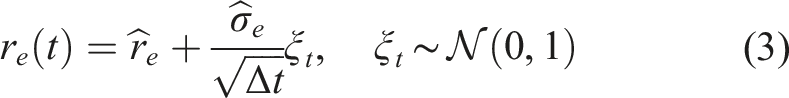
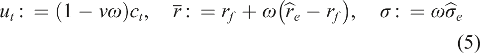
In this paper, we consider contribution policies parameterized in terms of an initial contribution rate u₀ and a growth rate ξ:

$u_t=u_0{e}^{\xi t}$

(6)

so that u₀ and ξ are now the constrained decision variables for the planner. In what follows we assume that u₀ > 0 and ξ ≥ 0. The growth rate ξ can be tuned to compensate for inflation or increase future contributions, assuming that the net investable income will grow in the future.

2.2. Stochastic Verhulst Equation and Langevin Dynamics

Note that equation (4) is a controlled SDE where control variables are u₀ and ξ. To simplify these dynamics, we introduce a new dimensionless variable v _t defined as follows:

$v_t=\frac{2}{{\sigma }^2}\frac{u_t}{{\mathrm{\Pi }}_t}=\frac{2}{{\sigma }^2}\frac{u_0{e}^{\xi t}}{{\mathrm{\Pi }}_t},$

(7)

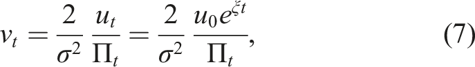
Note that the new variable v _t blends together the state variable Π _t and action variable u _t . Using Itô’s lemma, we obtain the SDE for v _t :

$d{v}_t=v_t\left(\xi -\overline{r}+{\sigma }^2-\frac{{\sigma }^2}{2}{v}_t\right)dt+\sigma v_{t}d{W}_t$

(8)

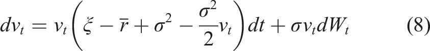
The new SDE for s _t does not depend on u₀, which is now embedded into the problem via the initial value v₀. ⁴ The only remaining control parameter explicitly appearing in (8) is ξ.

The SDE (8) is known in the literature as the stochastic Verhulst equation, see e.g., Giet et al. (2015). Recently, the SDE (8) with time-dependent coefficients was proposed by Itkin et al. (2021) as an attractive model of short interest rates that addresses some deficiencies of the classical Black-Karasinski model. Furthermore, they developed a method of solving the BKE for the SDE (8) with general time-dependent coefficients using an original integral transform method (Itkin et al., 2022). The method of Itkin et al. (2021) could be considered as an alternative approach to the semi-analytical method developed in this paper, see also the summary section for further comments. ⁵

To transform the multiplicative noise in the resulting SDE into an additive noise, we apply one more transformation to a new variable x _t :

$x_t=-\hspace{0.17em}\log \hspace{0.17em}{v}_t$

(9)

so that $v_t=e^{-x_t}$ . The SDE for x _t reads

$\begin{array}{ll}d{x}_t=-\left(\eta -\frac{{\sigma }^2}{2}{e}^{-x}\right)dt+\sigma d{W}_t,& \eta :=\xi -\overline{r}+\frac{{\sigma }^2}{2}\end{array}$

(10)

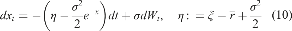
The new parameter η introduced in the SDE (10) can be used as a new control variable in lieu of ξ, with constraints inherited from constraints on ξ.

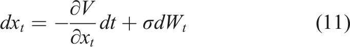
Now, the SDE (10) can be viewed as an (overdamped) Langevin equation

$d{x}_t=-\frac{\partial V}{\partial x_t}dt+\sigma d{W}_t$

(11)

where the potential function V = V(x) is defined as follows:

$V\left(x\right)=\eta x+\frac{{\sigma }^2}{2}{e}^{-x}$

(12)

and we use the short notation $\partial V/\partial x_t:={\partial V/\partial x|}_{x=x_t}$ . Note that parameter η becomes a control parameter for the Langevin potential V(x).

Consider now the conditional tail probability $p\left(w,t\right):=P^{\left(\pi \right)}\left[{\mathrm{\Pi }}_T<\widehat{\mathrm{\Pi }}|{\mathrm{\Pi }}_t=w\right]$ , where Π _T stands for the terminal wealth at time T, $\widehat{\mathrm{\Pi }}$ is a target wealth, and the notation $P^{\left(\pi \right)}[\cdots ]$ is introduced to emphasize the dependence of this conditional probability on the policy π≔(u₀, ξ). Our problem amounts to the task of choosing optimal values of u₀ and ξ such that the conditional tail probability p(v, 0) as seen now at time t = 0 does not exceed a certain target probability level α such as α = 5%. Now, when conditioning on the policy π≔(u₀, ξ), we can equivalently compute the tail probability p(v, t) in terms of variables v _t and x _t introduced above. Denoting corresponding target variables computed according to equations (7) and (9) as $\widehat{v}$ and $\widehat{x}$ , we can write down the following chain of equations:

$P^{\left(\pi \right)}\left[{\mathrm{\Pi }}_T\le \widehat{\mathrm{\Pi }}|{\mathrm{\Pi }}_t=w\right]=P^{\left(\pi \right)}\left[v_T\ge \widehat{v}|v_t=v\right]=P^{\left(\pi \right)}\left[x_T\le \widehat{x}|x_t=x\right]$

(13)

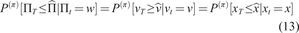
This shows that the tail probability $P^{\left(\pi \right)}\left[{\mathrm{\Pi }}_T\le \widehat{\mathrm{\Pi }}|{\mathrm{\Pi }}_t=w\right]$ of the original problem can be equivalently computed using the variable x _t . As will be shown next, the advantage of doing this is that using the variable x _t , our problem has a semi-analytical solution.

2.3. From the Fokker-Planck-Kolmogorov Control to the Schrödinger Control

While the Langevin equation (11) provides the path-wise description of stochastic dynamics, a corresponding probabilistic formulation is given by the FPE for the probability density f(x, t):

$\frac{\partial f\left(x,t\right)}{\partial t}=\frac{\partial }{\partial x}\left[\frac{\partial V}{\partial x}f\left(x,t\right)\right]+\frac{{\sigma }^2}{2}\frac{{\partial }^{2}f\left(x,t\right)}{\partial x^2}$

(14)

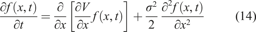
The probability density f(x, t) that solves the FPE equation is a distribution of x _t at time t given controls (u₀, η). To ease the notation, the dependence on controls is suppressed in all relations in this section.

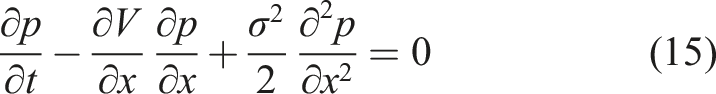
The second probability function we consider is the tail probability $p\left(x,t\right):=P^{\left(\pi \right)}\left[x_T\le \widehat{x}|x_t=x\right]$ . It satisfies the BKE:

$\frac{\partial p}{\partial t}-\frac{\partial V}{\partial x}\frac{\partial p}{\partial x}+\frac{{\sigma }^2}{2}\frac{{\partial }^{2}p}{\partial x^2}=0$

(15)

with the terminal condition

$\begin{array}{ll}p\left(x,T\right)=\theta \left(\widehat{x}-x\right),& \widehat{x}:=\log \frac{\mathrm{\hslash }\widehat{\mathrm{\Pi }}}{2u_0{e}^{\xi T}}\end{array}$

(16)

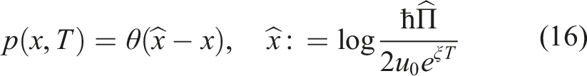
Let us look for solutions of the FPE (14) and BKE (15) in the following form:

$\begin{array}{lll}f\left(x,t\right)& =& e^{-\frac{V\left(x\right)}{\mathrm{\hslash }}}\mathrm{\Psi }\left(x,t\right),\mathrm{\hslash }:={\sigma }^2\\ p\left(x,t\right)& =& e^{\frac{V\left(x\right)}{\mathrm{\hslash }}}\overline{\mathrm{\Psi }}\left(x,\tau \right),\tau :=T-t\end{array}$

(17)

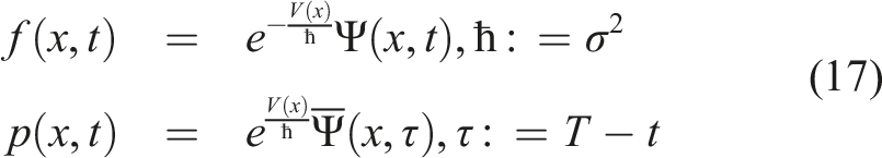
Here we introduced a new parameter ℏ = σ² to make formulae to follow look more familiar. Also note the time reversal t → τ = T − t in the second relation.

Substituting these expressions back into equations (14) and (15), we obtain a pair of PDEs for Ψ(z, t) and $\overline{\mathrm{\Psi }}\left(z,\tau \right)$ :

$-\mathrm{\hslash }\frac{\partial \mathrm{\Psi }\left(x,t\right)}{\partial t}=\left[-\frac{{\mathrm{\hslash }}^2}{2}\frac{{\partial }^2}{\partial x^2}+U\left(x\right)\right]\mathrm{\Psi }\left(x,t\right)$

(18)

$-\mathrm{\hslash }\frac{\partial \overline{\mathrm{\Psi }}\left(x,\tau \right)}{\partial \tau }=\left[-\frac{{\mathrm{\hslash }}^2}{2}\frac{{\partial }^2}{\partial x^2}+U\left(x\right)\right]\overline{\mathrm{\Psi }}\left(x,\tau \right)$

(19)

where

$U\left(x\right)=\frac{1}{2}{\left(\frac{\partial V}{\partial x}\right)}^2-\frac{\mathrm{\hslash }}{2}\frac{{\partial }^{2}V}{\partial x^2}$

(20)

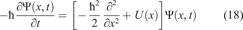
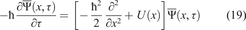
Written in this form, equations (18) and (19) should look very familiar to the reader acquainted with quantum mechanics. Equation (18), formulated in time t, is the Schrödinger equation in Euclidean (imaginary) time with the ‘Planck constant’ ℏ = σ² and potential U(x). On the other hand, equation (19) is the Schrödinger equation in backward time τ = T − t. In what follows, we will refer to equations (18) and (19) as, respectively, the Fokker-Planck Schrödinger equation (FP-SE), and the backward Kolmogorov Schrödinger equation (BK-SE).

Note that while the FP-SE (18) and BK-SE (19) have identical forms, they satisfy different initial conditions:

$\begin{array}{ll}\mathrm{\Psi }\left(x,0\right)=e^{\frac{V\left(x\right)}{\mathrm{\hslash }}}\delta \left(x-x_0\right),& \overline{\mathrm{\Psi }}\left(x,0\right)=e^{-\frac{V\left(x\right)}{\mathrm{\hslash }}}\theta \left(\widehat{x}-x\right)\end{array}$

(21)

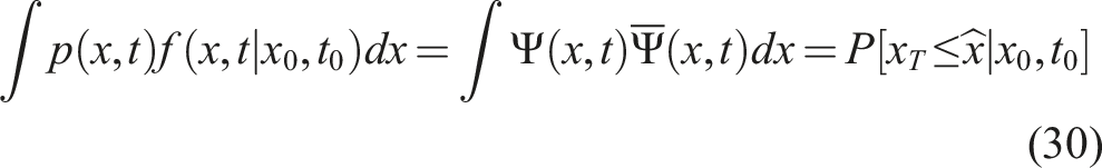
This implies that e^−V(x)/ℏΨ(x, t) is the Green’s function for equation (19), and therefore, we can relate the two functions as follows:

$\overline{\mathrm{\Psi }}\left(x,T\right)={\int }_{-\infty }^{\infty }d{x}^{\prime }{e}^{-\frac{V\left(x^{\prime }\right)}{\mathrm{\hslash }}}\overline{\mathrm{\Psi }}\left(x^{\prime },0\right)\mathrm{\Psi }\left(x,T|x^{\prime },0\right)$

(22)

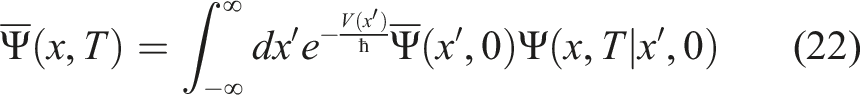
Using equation (17), this relation is seen to be equivalent to the conventional Feynman-Kac expression for the tail probability p(x, 0):

$p\left(x,0\right)=e^{\frac{2V\left(x\right)}{\mathrm{\hslash }}}{\int }_{-\infty }^{\infty }d{x}^{\prime }{e}^{-\frac{2V\left(x^{\prime }\right)}{\mathrm{\hslash }}}\theta \left(\widehat{x}-x^{\prime }\right)f\left(x,T|x^{\prime },0\right)$

(23)

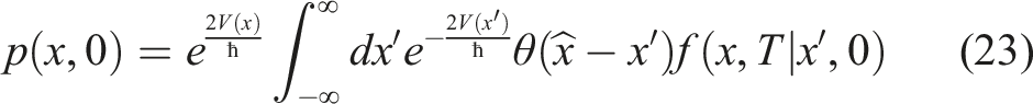
While the Feynman-Kac formula (23) gives one representation of a solution to our problem, an alternative approach is to directly solve the SE (19) with the initial condition stated in (21). As equations (18) and (19) have the same Hamiltonian, their solutions can be found by expanding in the same set of basis functions. Therefore, it might be more convenient to directly solve the the BK-SE (19) because it does not involve an extra integration step of the Feynman-Kac representation (23), at least formally. ⁶

2.4. The Morse Potential

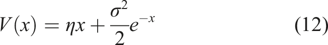
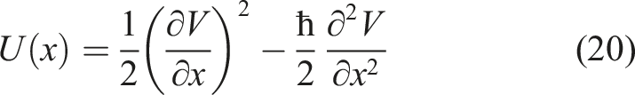
The Schrödinger potential (20) for our problem is obtained using equation (12):

$U\left(x\right)=D_0{\left(1-\frac{1}{g}{e}^{-x}\right)}^2+U_0$

(24)

where we defined the following parameters:

$\begin{array}{lll}g:=1+\frac{2\eta }{\mathrm{\hslash }}=2\left(1+\frac{\xi -\overline{r}}{\mathrm{\hslash }}\right),& D_0:=\frac{{\mathrm{\hslash }}^2}{8}{g}^2,& U_0:=-\frac{{\mathrm{\hslash }}^2}{8}\left(2g-1\right)\end{array}$

(25)

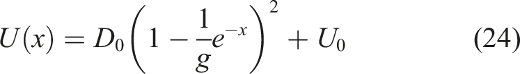
The control variable ξ of the original problem is now embedded into the ‘coupling constant’ parameter g of the corresponding quantum mechanical problem (18) or (19). The original control problem therefore becomes a problem of quantum control for the Euclidean quantum mechanics. In this problem, we control the coupling constant g of the quantum mechanical potential U(x) and the initial position of a quantum mechanical ‘particle’ representing the wealth of the planner in such a way that the terminal WF $\overline{\mathrm{\Psi }}\left(x,T\right)$ is driven to a desired form.

In its turn, the coupling constant g determines the degree of non-linearity of potential U(x). If g > 0, the potential has a minimum at x = − log  g. In the limit g → 0, the minimum is pushed to infinity, and we obtain $U\left(x\right)=\left({\mathrm{\hslash }}^2/8\right)\left(1+e^{-2x}\right)$ , i.e., the potential becomes a monotonically decreasing function. In the opposite limit g → ∞, the potential U(x) becomes a constant U(x) = D₀ + U₀. For g < 0, the potential U(z) has no minima or maxima, and becomes a monotonically decreasing function.

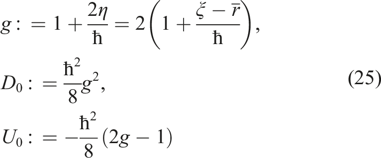
The potential U(x) can be written more compactly once we differentiate between two possible regimes g > 0 and g < 0 of the model. Introducing parameter $x_{\star }$ := − log  |g|, we can write the potential U(x) in the following form:

$\begin{array}{ll}U\left(x\right)=\{\begin{array}{l}{D}_0{\left(1-e^{-\left(x-x_{\star }\right)}\right)}^2+U_0,\\ D_0{\left(1+e^{-\left(x-x_{\star }\right)}\right)}^2+U_0,\end{array}& \begin{array}{ll}\text{if}& g>0\\ \text{if}& g<0\end{array}\end{array}$

(26)

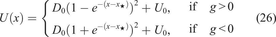
Focusing on the first expression here obtained for g > 0, this is the celebrated Morse potential known from quantum mechanics, see Landau and Lifschitz (1980), see Figure 1. As this potential is very tractable, the reduction of our initial financial problem to Schrödinger equations (18) and (19) with the Morse potential U(x) is very helpful. More specifically, it enables semi-analytical solutions for both Schrödinger equations (18) and (19), and hence for both the FPE (14) and BKE (15) by virtue of equation (17). ⁷ We only give here the final expressions for the FPE and BKE solutions f(x, t) and p(x, t). Details are left to Appendix A which is written in a reasonably self-contained way to provide a brief overview of these methods for the reader without a background in theoretical physics.

Figure 1.

Examples of the Morse potential for different values of parameter g driven by different values of control parameter ξ. Both potentials have a minimum at 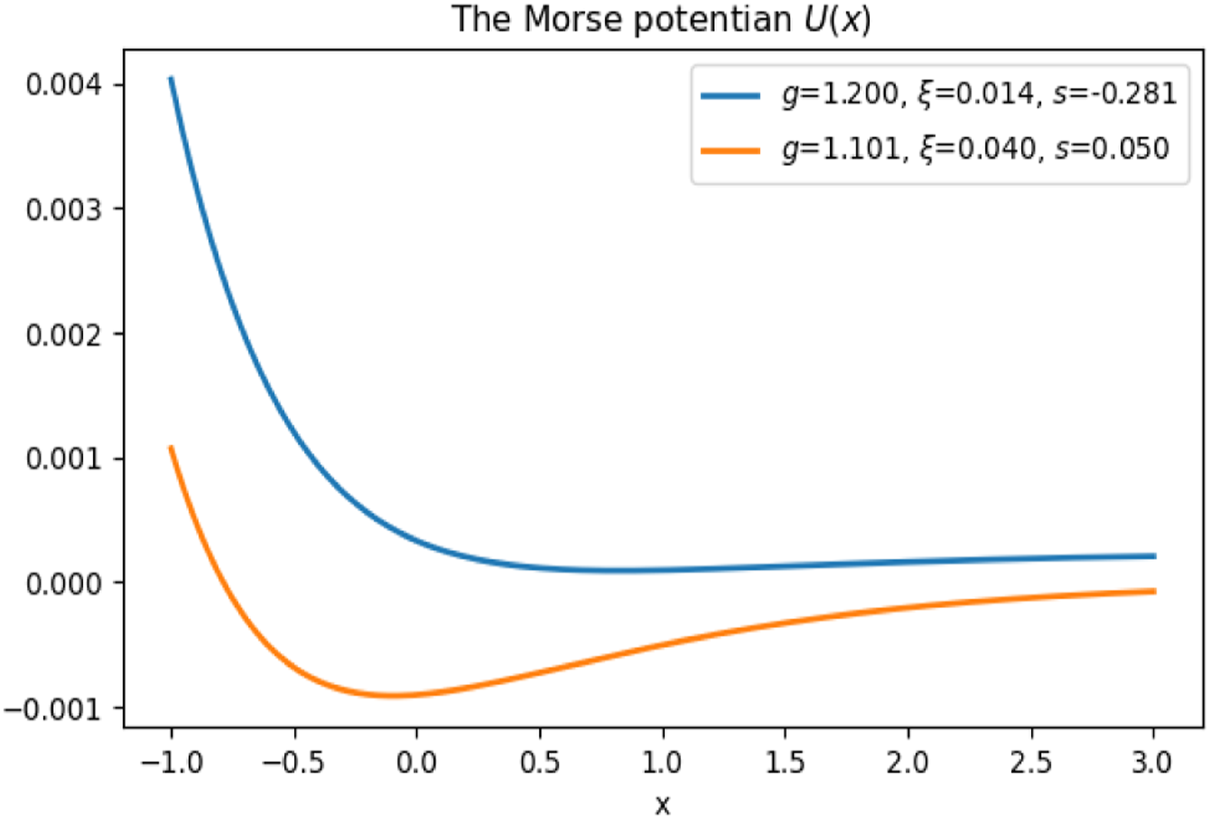$x_{\star }$ = − log(g) where g = 2s + 1. For small values of ξ, the potential well becomes very shallow. If ξ becomes smaller than ${\xi }_{low}:=\overline{r}-{\sigma }^2$ , the minimum disappears, and the potential becomes monotonically decreasing. For larger values of ξ, the minimum becomes more pronounced.

The solution presented in Appendix A shows that both functions Ψ(x, t) and $\overline{\mathrm{\Psi }}\left(x,t\right)$ depend on x only through the so-called Morse variable y≔e^−x, so that we can equivalently write them as $\mathrm{\Psi }\left(y,t\right),\overline{\mathrm{\Psi }}\left(y,t\right)$ . Recalling equation (9), the time-t Morse variable value y _t can be expressed in terms of the original model inputs:

$y_t=e^{-x_t}=\frac{2u_0{e}^{\xi t}}{\mathrm{\hslash }{\mathrm{\Pi }}_t}$

(27)

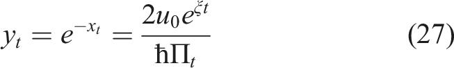
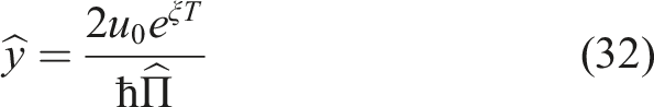
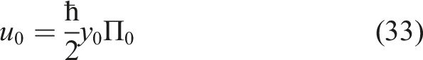
If we use this relation for t = 0, it means that the initial value y₀ at time zero is simply the initial contribution u₀ scaled by the portfolio value Π₀ and portfolio variance ℏ = σ². In other words, y₀ can be viewed as a correct dimensionless version of the initial control u₀ (which has the dimension of dollars per year) which enables a meaningful comparison of different plans and different market conditions. For this reason, in most of our numerical examples to follow we will use the initial value y₀ of the Morse variable as a dimensionless control parameter in lieu of the initial control parameter u₀.

As $\mathrm{\Psi }\left(x,t\right),\overline{\mathrm{\Psi }}\left(x,t\right)$ are functions of the Morse variable y, it is convenient to reformulate equation (17) in terms of the Morse variable y = e^−x. For the exponential factor e^−V(x)/ℏ, it gives

$e^{-V\left(y\right)/\mathrm{\hslash }}={e^{-V\left(x\right)/\mathrm{\hslash }}|}_{x=-\hspace{0.17em}\log \hspace{0.17em}y}=y^{\eta /\mathrm{\hslash }}{e}^{-y/2}$

(28)

Changing the variables in equation (17) to the Morse variable y = e^−x, we write them as follows ⁸

$\begin{array}{lll}f\left(y,t\right)& =& y^{-1}{e}^{-V\left(y\right)/\mathrm{\hslash }}\mathrm{\Psi }\left(y,t\right)=y^{\eta /\mathrm{\hslash }-1}{e}^{-y/2}\mathrm{\Psi }\left(y,t\right)\\ p\left(y,t\right)& =& e^{V\left(y\right)/\mathrm{\hslash }}\overline{\mathrm{\Psi }}\left(y,\tau \right)=y^{-\eta /\mathrm{\hslash }}{e}^{y/2}\overline{\mathrm{\Psi }}\left(y,\tau \right)\end{array}$

(29)

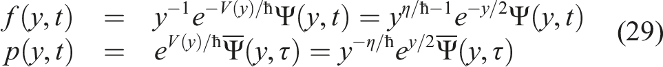
The explicit form of the FP-SE WF Ψ(y, t) and the BK-SE WF $\overline{\mathrm{\Psi }}\left(y,t\right)$ is given in equations (A51) and (A52), respectively.

In Figure 2, we show 3D views of the WF $\overline{\mathrm{\Psi }}\left(y,T\right)$ and the BKE density p(y, 0) as a function of two variables y = y₀ and ξ for a typical retirement plan with the horizon T = 20Y for the target wealth of $2.5m, initial wealth of $0.5m, and portfolio volatility of 30%, with the following bounds on admissible values of u₀ and ξ: $10k $\le u_0\le$ $100K, and 2.5% ≤ ξ ≤ 5.0%. This parameter and constraints settings will also be used below in other examples illustrating the working of the model.

Figure 2.

On the left: The WF 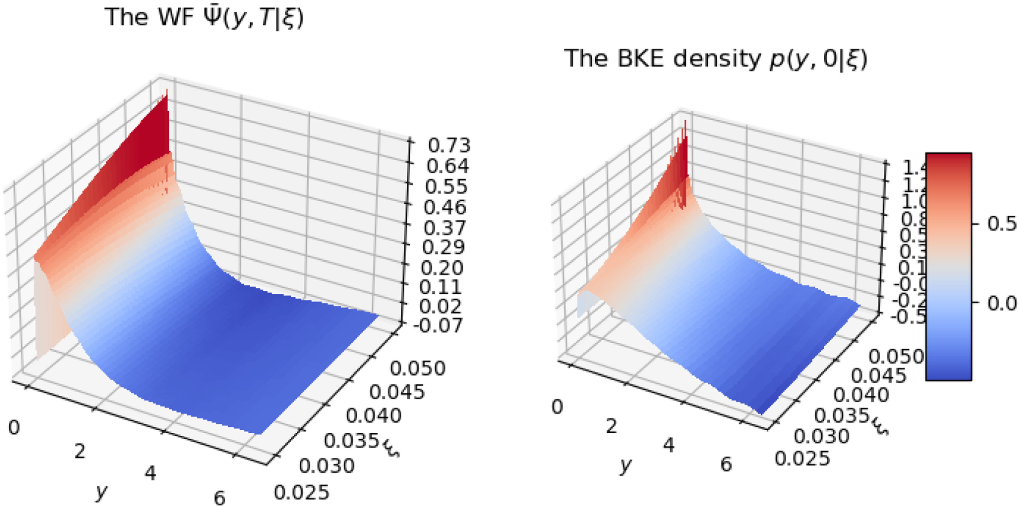$\overline{\mathrm{\Psi }}\left(y,T\right)$ for T = 20, shown as a function of both y and ξ using N = 150 basis functions, for a retirement plan with the horizon T = 20Y, the target wealth of $2.5m, the initial wealth of $0.5m, and portfolio volatility of 30%, with the following bounds on admissible values of u₀ and ξ: $10k $\le u_0\le$ $100K, and 2.5% ≤ ξ ≤ 5.0%. On the right: the corresponding BKE tail probability p(y, 0).

Note that using equation (29), we can obtain the Chapman-Kolmogorov equation in terms of Ψ(x, t) and $\overline{\mathrm{\Psi }}\left(x,t\right)$ :

$\int p\left(x,t\right)f\left(x,t|x_0,t_0\right)dx=\int \mathrm{\Psi }\left(x,t\right)\overline{\mathrm{\Psi }}\left(x,t\right)dx=P\left[x_T\le \widehat{x}|x_0,t_0\right]$

(30)

which resembles the normalization condition $\int {\left|\mathrm{\Psi }\left(x,t\right)\right|}^{2}dx=1$ in quantum mechanics.

3. Optimization of Contribution Policy: Efficient Frontiers

Optimization of contribution policy is performed using the semi-analytical solution given by the second equation in equation (29) which gives the tail probability of the event ${\mathrm{\Pi }}_T<\widehat{\mathrm{\Pi }}$ in terms of the tail probability of the Morse variable y:

$P\left[{\mathrm{\Pi }}_T\le \widehat{\mathrm{\Pi }}|{\mathrm{\Pi }}_t,u_t\right]=P\left[y_T\ge \widehat{y}|y_t,\xi \right]=y^{-\eta /\mathrm{\hslash }}{e}^{y/2}\overline{\mathrm{\Psi }}\left(y,t|\xi \right)$

(31)

Here $\widehat{y}$ is the target value of the Morse variable y, which is computed according to equation (27):

$\widehat{y}=\frac{2u_0{e}^{\xi T}}{\mathrm{\hslash }\widehat{\mathrm{\Pi }}}$

(32)

and we wrote the WF $\overline{\mathrm{\Psi }}\left(y,t\right)$ as $\overline{\mathrm{\Psi }}\left(y,t|\xi \right)$ to emphasize its dependence on ξ.

Our strategy for optimization of contribution policy is to compute equation (31) for all possible values of control variables u₀ and ξ, and then find the optimal control that matches the threshold value for the BKE tail probability p(y, 0). In practice, this involves computing the tail probability (31) for all nodes of a certain two-dimensional grid for u₀ and ξ, and then interpolating to other values of u₀, ξ using splines. As in the range of input parameter that have practical interest the model behaves in a very smooth way (see Figure 2), this means that we can use a rather small grid of pairs (u₀, ξ) to perform accurate spline interpolation.

Furthermore, the mathematical structure of the solution to our problem suggests that instead of considering the pair (u₀, ξ) as independent controls, we can equivalently but more conveniently map them onto the pair (y, ξ). As suggested by equation (27), y is the right dimensionless version of u₀, additionally scaled by the portfolio volatility, therefore using variable y instead of the absolute dollar amount u₀ enables comparing different plans and different market conditions. If the current time is set to zero and the initial wealth Π₀ is fixed, then values of u₀ corresponding to values of y = y₀ are obtained according to (27):

$u_0=\frac{\mathrm{\hslash }}{2}{y}_0{\mathrm{\Pi }}_0$

(33)

In our numerical examples presented below, we use a non-uniform grid ⁹ of values of y of size 100. In addition, we use 20 grid points to represent possible values of ξ. The values of the BKE density for arbitrary intermediate inputs are obtained using the standard 2D cubic splines.

As the inputs (ξ, y) (or equivalently (ξ, u₀)) form a 2D plane, equation (31) implies that the problem of finding the optimal contributions $u^{\star }=\left(u_0^{\star },{\xi }^{\star }\right)$ for a plan with the goal wealth $\widehat{\mathrm{\Pi }}$ that we want to exceed with probability equal to 1 − α amounts to solving the equation

$P\left[y_T>\widehat{y}|y_t,{\xi }_t,t\right]=\alpha$

(34)

in this 2D (ξy)-plane.

Note that we call here an optimal solution $u^{\star }=\left(u_0^{\star },{\xi }^{\star }\right)$ is in fact a satisficing solution: we do not want to drive the tail probability (34) all the way down to zero, we only need to drive it below the target confidence level α. Satisficing decision-making is different from decision-making based on maximization of a total reward as is done in DP or RL. Indeed, with DP or RL, a reasonably-behaved value function should have a global maximum, therefore there should be at least one policy that leads to such maximum value. Quite differently, with satisficing decision-making problems such as our equation (34), solutions for feasible problems form contour lines on the surface of BKE density p(y, 0|ξ).

We will refer to such contour lines at different probability levels as efficient frontiers, similarly to the use of this term in the Markowitz (1952) portfolio theory (Markowitz, 1952). The 3D plot of the BKE tail probability p(y, 0|ξ) as a function of both controls y and ξ with efficient frontier lines is shown in Figure 3. The corresponding 2D view that might be easier for analysis is shown in Figure 4.

Figure 3.

3D plot of the BKE tail probability p(y, 0|ξ) viewed as a function of both control variables y and ξ, along with efficient frontier lines corresponding to probability confidence levels α = [3, 5, 7.5, 10, 15, 20]%.

Figure 4.

The 2D view of efficient frontier lines in the 3D space in Figure 3. Lines in the (ξy)-plane labeled by numbers and colors are efficient frontiers of the planning problem at the confidence levels α marked on the curve. For any fixed value of α, any point on a line is as good as any other point in terms of the quality of the solution obtained with the model. Further preferences may be based on other considerations that were not used as a part of model inputs.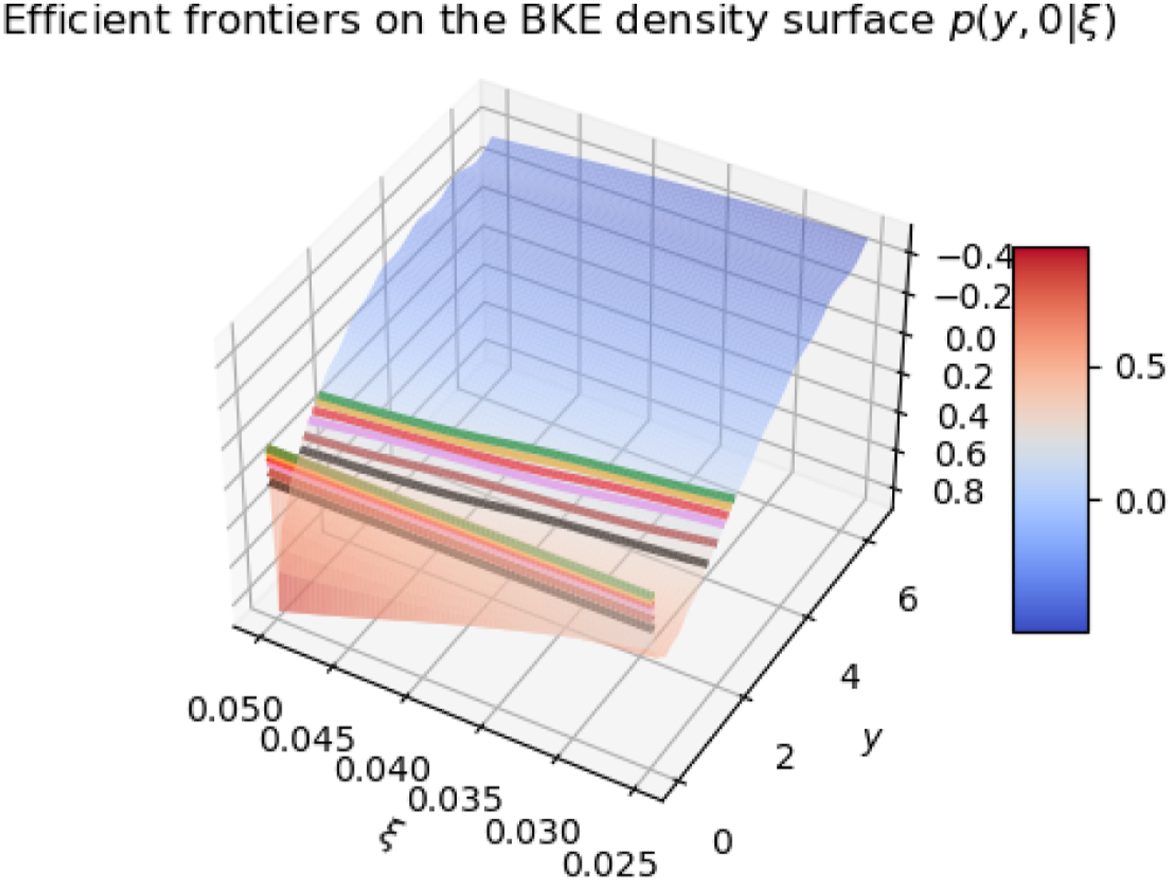

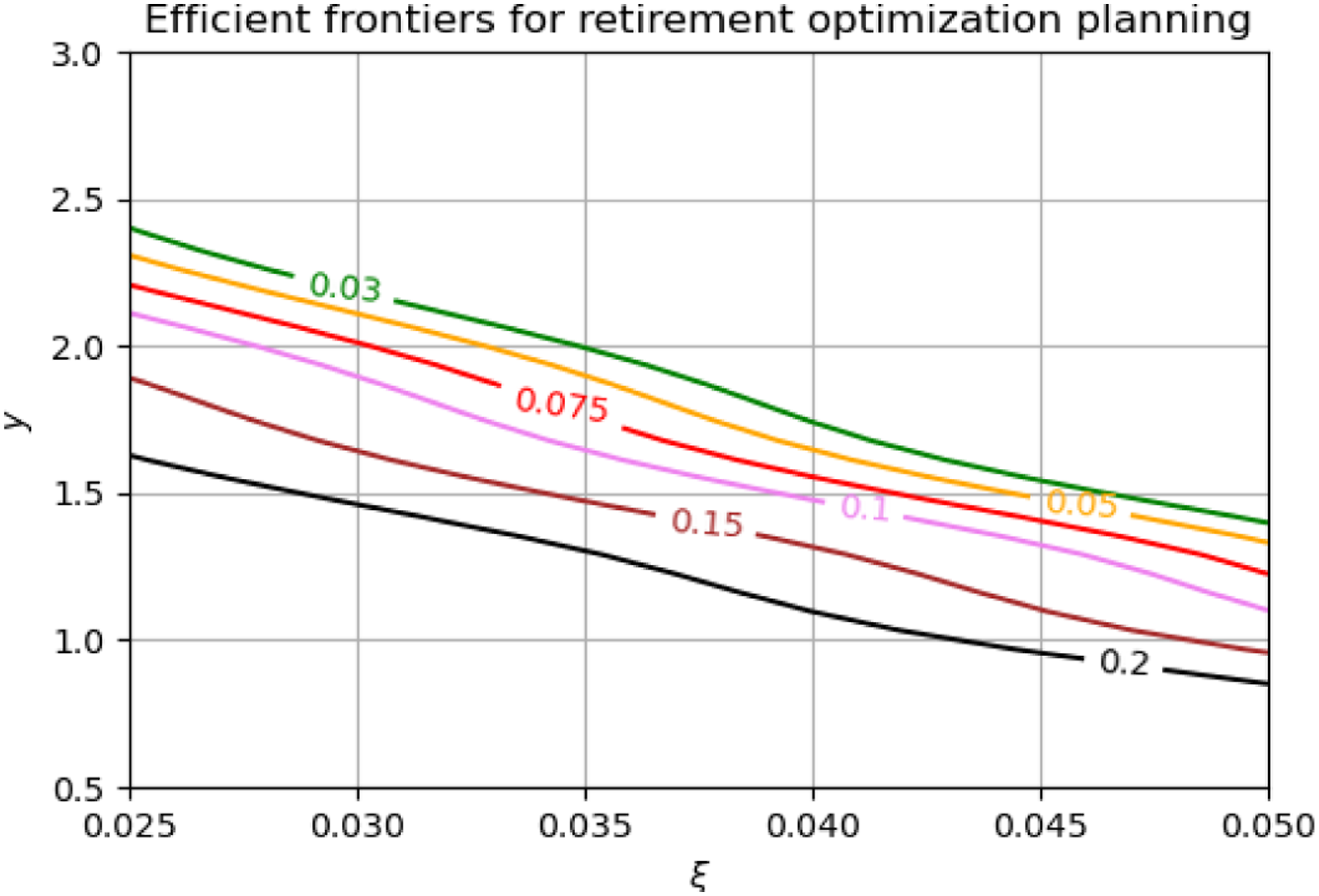
Efficient frontier lines shown in Figures 3 and 4 can be used for visualization of all possible optimal policies at different confidence levels α for a given plan with user-defined initial and target wealth levels and constraints on admissible values of control parameters. Note that while our original objective was formulated as an optimization problem, the solution presented here reduces to a combination of a 2D cubic spline and a root-finding, or equivalently a contour construction algorithm. ¹⁰ The plan optimization part thus reduces to the task of drawing a constant-probability line on a computed solution surface given by the BKE density p(y, t|ξ).

4. Summary

This paper addresses a problem that is routinely solved (or at least supposed to be routinely solved) by millions of working individuals who participate in retirement saving plans such as the 401(K) plans in the US, or similar programs worldwide. The problem is to plan an optimal contribution schedule to their investment portfolio so that their wealth by the time of retirement will be above a certain target wealth level at a certain probability confidence level.

While his problem appears to be entirely unrelated to any sort of quantum physics, what we proposed in this paper is that in fact, this problem is quantum mechanics in disguise! This of course does not mean quantization of the retirement wealth, or (unfortunately!) a teleportation to a wealthier quantum state, or anything of this sort that can come to the minds of non-physicists when they hear the words ‘quantum mechanics’ or ‘Schrödinger equation’. What we mean by saying “retirement planning is quantum mechanics in disguise” rather refers to the fact that, with standard simplifications and assumptions of normal equity returns etc., the first problem is mathematically identical to a very famous problem in quantum mechanics, namely quantum mechanics with the Morse potential.

It is interesting to note here that the non-linear Morse potential (26) arises in our approach due to the mere presence of controls (u₀, ξ). Indeed, if we take u _t = 0 in equation (4), we end up with the standard Geometric Brownian Motion (GBM) model as a model of the portfolio wealth process. This can be contrasted with scenarios where the uncontrolled dynamics are non-linear due to a non-linear potential. Models of non-linear dynamics for equity stock markets with nonlinearity generated by market flows and market frictions have been previously proposed by the author in (Halperin, 2021, 2022). In contrast, in this paper we start with linear uncontrolled dynamics of the GBM model, while non-linearities arise in the mathematically equivalent formulation of the problem based on a transition to the Morse variable y that blends together the state and action variables.

Our method can be compared with the conventional feedback-loop control approach of DP or RL. It is well known that low dimensional problems with continuous controls can be efficiently solved by discretization of action variables. Therefore, the mere fact of reducing our 2D control problem to a 2D grid search problem may be hardly surprising on its own. Nonetheless, for practical applications that we have in mind for this paper, the end criteria of success are the accuracy and the speed of calculation. The approach of this paper can be viewed as a way to efficiently construct a grid of policies and value functions (i.e., BKE tail probabilities, in our case) using methods that work in physics.

While our step of constructing a grid of controls and output BKE tail probabilities is similar to the procedure employed in DP and RL upon discretization of action variable, one important difference of our scheme from DP or RL is what we do next with this grid. With DP or RL, we want to find a policy (i.e., a grid point) where the value function attains its global maximum - which can be performed via a regular grid search because of discretization. In contrast, with goal-based wealth management, our setting fits the framework of satisficing decision-making of Simon (1955, 1979). This is because with goal-based wealth management, we want to find a policy that is good enough (i.e., satisficing) to drive the probability of the terminal portfolio wealth falling below some target value $\widehat{\mathrm{\Pi }}$ to the level of α, but not below! This is not a maximization problem that is usually solved by DP or RL, this is a problem of finding contour lines on a surface of the BKE tail probability. Therefore, the nature of a solution for DP or RL is quite different from a solution to satisficing decision making: while the solution is given by a point in an action space for the former, it has a form of a degenerate contour line for the latter.

One important concept that we propose here as a way to communicate the model results to end users is the notion of efficient frontiers - constant probability level curves on the surface of the BKE tail probability p(y, 0|ξ) viewed as a function of control parameters y and ξ. Note here that most of RL methods typically provide a single point in a multi-dimensional action space as an optimal solution to a stochastic control problem. While the present paper emphasizes the importance of continuous degenerate families of solutions (efficient frontiers) for our particular 2D control problem with a satisficing objective function, the author is unaware of any systematic discussion of degenerate satisficing solutions in a general RL setting.

Back to the mathematical identity of the retirement planning problem to the quantum mechanical problem, note that we reduced our initial problem not just to the standard textbook problem of solving the Schrödinger equation with a fixed Morse potential, but rather to a quantum optimal control problem with the Morse potential. Unlike the passive dynamics problem of the conventional quantum mechanics, in tasks of quantum control, the objective is to control the Schrödinger potential in order to bring a quantum system into a desired terminal state at a smallest cost or in a shortest time. In the same way, here we control the degree of non-linearity of the Morse potential and the initial particle position in order to achieve a desired quantum mechanical terminal state $\overline{\mathrm{\Psi }}\left(y,T\right)$ . In this sense, the proposition formulated in the beginning of this section can be refined to the following proposition:

The wealth management problem is a quantum optimal control problem in disguise.

where, as before, by saying in disguise we mean mathematically equivalent. A recent work applied quantum computing to quantum mechanics of molecules with the Morse potential to compute energies of two lowest eigenstates by Apanasevich et al. (2021). Exploring potential applications of quantum computing to the problem formulated in this paper and its potential extensions can be an interesting venue for future research.

Another interesting direction would be to explore alternative methods for the FPE and BKE equations which may or may not make connections to the Schrödinger equation as we did in this paper. While here we solved the BKE equation and its associated Schrodinger equation using the standard eigenvalue decomposition method coupled with a non-standard way of constructing the basis, this is clearly not the only available, and likely not the most efficient way to solve these equations. In particular, it would be interesting to apply the integral transform approach of Ref. Itkin et al. (2021) in our setting of optimal control. Finally, extensions to multiple dimensions can be another interesting topic for future research along the lines proposed in this paper.