Sage Journals: Discover world-class research

Abstract

Quantum computers are expected to contribute more efficient and accurate ways of modeling economic processes. Quantum hardware is currently available at a relatively small scale, but effective algorithms are limited by the number of logic gates that can be used, before noise from gate inaccuracies tends to dominate results. Some theoretical algorithms that have been proposed and studied for years do not perform well yet on quantum hardware in practice. This encourages the development of suitable alternative algorithms that play similar roles in limited contexts. This paper implements this strategy in the case of quantum counting, which is used as a component for keeping track of position in a quantum walk, which is used as a model for simulating asset prices over time. We introduce quantum approximate counting circuits that use far fewer 2-qubit entangling gates than traditional quantum counting that relies on binary positional encoding. The robustness of these circuits to noise is demonstrated. While this paper is mainly about robust simplified quantum circuit designs, we compare some aspects of the results with price change distributions from stock indices, and compare the behavior of circuits with and without mid-measurement to trends in the housing market.

Keywords

quantum circuits quantum approximate counting quantum walks quantum finance quantum asset pricing

1. Motivation: Quantum Finance Implementations in 2023

Quantum computers are expected to enable more sophisticated and accurate modeling of various financial situations. The reasons for the high expectations for quantum finance are in some cases thoroughly worked-out algorithmically: for example, Egger et al. (2020) survey applications including option pricing and risk management, where Monte Carlo simulation methods are commonly used, and explain how quantum algorithms for amplitude estimation offer a potential quadratic speedup (by reducing the number of samples needed for the variance of the probabilistic outcomes to converge). As with quantum factoring and search, there are solid reasons for expecting quantum computers to perform well at large-scale problems that are especially challenging for classical computing methods.

In some cases, the proposed models are simple and concise enough to be simulated on classical hardware, and now in the early 2020’s their behavior can be explored on real quantum computers. However, these models have been small. Using just a 2-qubit photonics processor, Qiang et al. (2016) were able to model a continuous time walk on a connected graph with 4 states. Stamatopoulos et al. (2020) used 3 superconducting qubits for option pricing and Zhu, Johri, et al. (2022) used 6 trapped-ion qubits to perform generative modeling for correlated stock prices.

The scale of such experiments has been particularly limited by qubit availability and quantum gate accuracy. For example, the 3-qubit circuit of Stamatopoulos et al. (2020) was optimized down to 18 2-qubit entangling gates and 33 single-qubit gates, but even with this small circuit, error rates in the results ranged from 62% raw, to 21% using Richardson extrapolation for error-correction. This is not surprising, since the accuracies of the single-and 2-qubit gates were estimated at 99.7% and 97.8% respectively, and .997³³ × .978¹⁸ ≈ .587, so the compounded gate error rate is at least 40%.

A safe implementation strategy might be to wait for large-scale fault-tolerant quantum computers to become available, but this runs the risk of missing opportunities in the meantime. Instead, researchers such as Stamatopoulos et al. (2020) and Zhu, Johri, et al. (2022) try to use currently-available quantum hardware, and ask whether implementations can be made robust enough to provide value sooner. In the current NISQ era (Noisy Intermediate-Scale Quantum), the scarce resources include the number of qubits, and also, as seen above, the number of gates, and especially the number of 2-qubit entangling gates. Circuits are sometimes described in terms of width (number of qubits) and depth (number of dates, or layers of gates), and both need to be minimized.

Quantum developers sometimes have many suggested designs to start from: quantum information processing has been explored as an academic field for some decades, and established literature provides many circuit recipes (Nielsen & Chuang, 2002). A natural strategy is to take such designs, consider their NISQ era limitations, and see if there are alternatives that provide some of the same functionality using fewer qubits or gates.

This paper develops some new examples of this approach, with the basic example of quantum counting. The central novel contribution of the paper are the approximate quantum counting circuits, introduced in Section 7. The motivation is that quantum counting is used as a component in the implementation of quantum random walks, which are proposed as a model for stock prices, and also for beliefs about the future value of stock prices, for the pricing of stock options. Beliefs are less exact than prices: it is not very important to make sure that an estimate of $1000 comes $1 after an estimate of $999 and $1 before an estimate of $1001; but it is important to make sure that these are all treated similarly, and that doubling any of them gives something in the region of $2000. The circuits proposed in this paper demonstrate such properties, albeit approximately, but much more accurately than is currently possible on quantum computers that use positional binary representations for numbers that strictly follow the axioms of arithmetic.

A distinct feature of quantum systems including quantum walks is that they behave differently when they are measured, compared to when they are left to evolve dynamically. Such behavior has been demonstrated with humans in psychology experiments (Kvam et al., 2015; Yearsley & Pothos, 2016), and is an important feature in quantum cognition and economics (Busemeyer & Bruza, 2012; Orrell, 2020). Section investigates the simulated behavior of the approximate counting circuits with mid-measurement, and shows that they exhibit desirable behavior (in this case, that more frequent measurement tends to reduce the chances of large changes). In a departure from many quantum cognition models, the macro effects of beliefs on transactions and prices cannot be described as the decision of particular cognitive agent, and it may be more appropriate to think of quantum models as representing the beliefs of whole groups of buyers and sellers, and measurements as decisions observed by the whole market. This theme is considered as part of introducing quantum walks in finance in Section 3, and the effects of measurement in Section 7, especially with reference to the housing market.

To begin with, the next few sections review some of the basic quantum logic gates and how they are put together into quantum circuits, the use of random walks and quantum walks in finance, and how these come together to emphasize the practical quantum counting problem.

2. Quantum Gates Used in this Paper

In mathematical terms, the key features that distinguish quantum from classical computers are superposition and entanglement. This section gives a brief summary of how these properties are worked with in quantum circuits. Some familiarity with quantum mechanics, especially Dirac notation, is assumed, so that |0⟩ and |1⟩ are the basis states for a single qubit whose state is represented in the complex vector space $C^{2}$ , a 2-qubit state is represented in the tensor product space $C^{2} \otimes C^{2} ≅ C^{4}$ with basis states |00⟩, |01⟩, |10⟩ and |11⟩, 3-qubit states are represented in $C^{\otimes 3} ≅ C^{8}$ with basis states |000⟩, |001⟩, …, |111⟩, and so on. For introductions to how linear algebra is written and used in quantum mechanics, see Nielsen and Chuang (2002, Ch 2), Orrell (2020, Ch 2). Quantum measurement is probabilistic: if |ϕ⟩ is an eigenvector of a given measurement operator, then a system in the state |ψ⟩ is observed to be in the state |ϕ⟩ with probability given by the square of their scalar product, ⟨ϕ|ψ⟩² (the Born rule), and if this outcome is observed, the system is now in the state |ϕ⟩.

Superposition can be realized in a single qubit: the state α|0⟩ + β|1⟩ is a superposition of the states |0⟩ and |1⟩, where α and β are complex numbers, with |α²| + |β²| = 1. Each single-qubit logic is a linear operator that preserves the orthogonality of the basis states and this normalization condition, and the group of such operators is U(2), the group of complex 2 × 2 unitary matrices. Single-qubit gates that feature prominently in this paper are shown in Figure 1. So single-qubit gates coherently manipulate the superposition state of an individual qubit.

Figure 1.

Some standard single-qubit gates and their corresponding matrices, which operate on the superposition state α|0⟩ + β|1⟩ written as a column vector (α,β)^T.

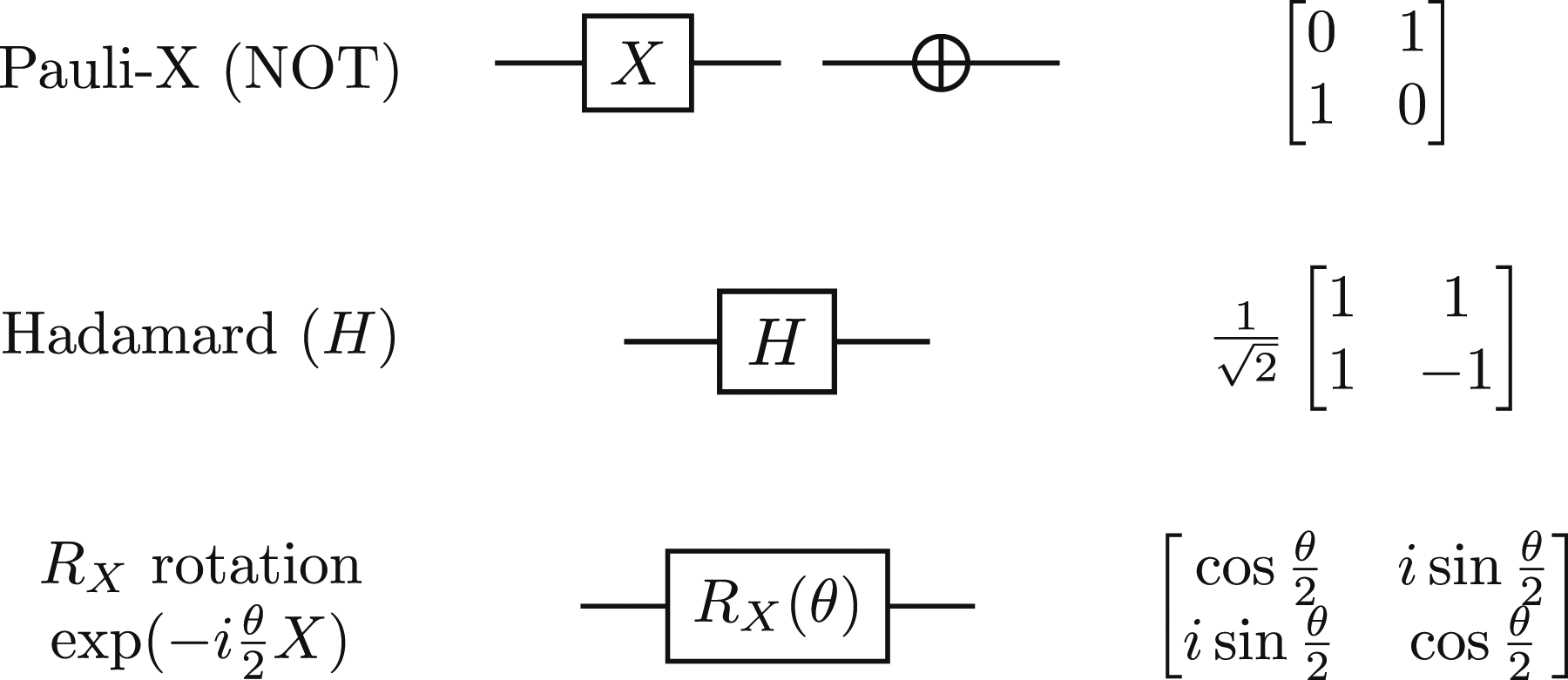
Entanglement is a property that connects different qubits. Since the 1930’s, quantum entanglement has gone from a hotly-disputed scientific prediction, to a statistical property demonstrated with large ensembles, to a connection created between pairs of individual particles, to a working component in quantum computers. All modern quantum computers have some implementation of an entangling gate, and only one kind is really needed, because all possible 2-qubit entangled states can be constructed mathematically by combining appropriate single-qubit gates before and after the entangling gate. Furthermore, a single 2-qubit entangling gate and a set of single-qubit gates forms a universal gateset for quantum computing (Nielsen & Chuang, 2002, §4.5).

The CNOT (controlled-NOT) gate of Figure 2 is the most common example of a 2-qubit gate in the literature. In the standard basis, its action is sometimes described as performing a NOT operation on the target qubit if the control qubit is in the |1⟩ state. Thus, as well as causing entanglement, it is sometimes thought of as a kind of conditional operator in quantum programming. Entanglement is the crucial property that distinguishes quantum computing algorithmically, because predicting the probability distributions that result from quantum operations with entanglement can become exponentially hard for classical computers. In simpler terms, quantum computing is special because it offers special kinds of interference, not because it offers special kinds of in-between-ness.

Figure 2.

The CNOT gate is a 2-qubit entangling gate, that acts upon the state α|00⟩ + β|01⟩ + γ|10⟩ + δ|11⟩. In the standard basis, its behavior can be described as “performing a NOT operation on the target qubit if the control qubit is in state |1⟩”.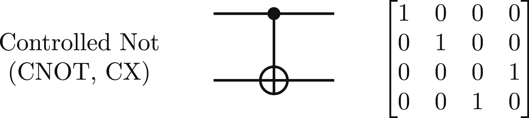

A quantum circuit consists of a register of qubits, and a sequence of logic gates that act on these qubits. For example, the circuit in Figure 3 prepares the famous Bell state (named after physicist John Bell, whose pioneering theorem motivated experiments that demonstrated real entanglement). It maps the input state |00⟩ to the state $1 / \sqrt{2} (| 00 〉 + | 11 〉)$ , which has the crucial ‘entangled’ behavior whereby if one qubit is measured to be in the |0⟩ state, the other qubit must also be in the |0⟩ state, and vice versa.

Figure 3.

Hadamard and CNOT gates in sequence make a quantum circuit that prepares the Bell state 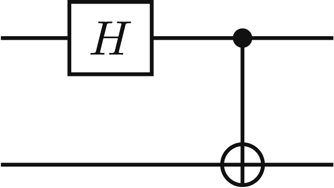$1 / \sqrt{2} (| 00 〉 + | 11 〉)$ .

Quantum circuits finish with measurements that record the 0 or 1 state of at least some of the qubits, and output this as classical information. (Some platforms also support measuring qubits before the end of a circuit.) The measurement outcomes are probabilistic, following the Born rule. A run of a single quantum circuit including outputting one sample of measurements is typically called a shot. Circuits are usually repeated several times, and the output counts from many individual shots are summarized into an output distribution. The process of running all the shots and gathering the outcomes is typically called a job.

There are many standard gate recipes and equivalences. In particular, larger operators are often thought of as distinct gates in their own right, an important example being the 3-qubit Toffoli gate of Figure 4. This is like an extended CNOT gate — it has 2 control qubits instead of 1, and performs an X-rotation/NOT operation on the target qubit if both the control qubits are in the |1⟩ state. The decomposition in Figure 4 shows that 5 CNOT gates are needed for each Toffoli gate. There are variants of this, but as a general rule-of-thumb, the error-rate of a Toffoli gate will be at least 4 times the error-rate of the 2-qubit gates form which it is assembled. Toffoli gates are particularly important for binary arithmetic, as seen in Section 5.

Figure 4.

The Toffoli gate diagram, showing that it performs a NOT operation on the target qubit if both the control qubits are in the |1⟩ state. On the right is one of its standard decompositions into CNOT and single-qubit gates, in which 5 CNOT gates are needed to implement one Toffoli gate.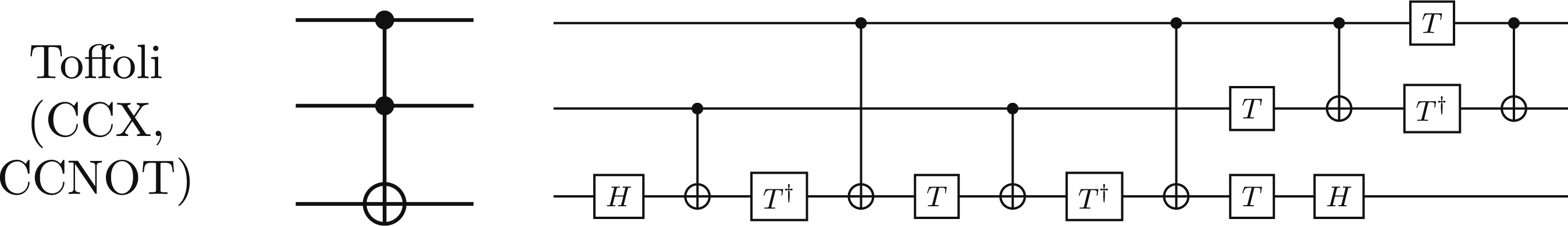

In the NISQ era, such considerations are pervasive: there is a ubiquitous tradeoff between circuit complexity (the number of gates needed to execute a given algorithm) and expected circuit accuracy (the more gates we use, the more inaccurate our results become).

3. Random Walks, Stock Prices, and Quantum Walks

This section briefly reviews the role of random walks and quantum walks in the modeling of asset prices. For a more thorough introduction, see Orrell (2020, Ch 7, 8). A random walk is a mathematical process that constructs a path through some base space composed of a succession of randomly-chosen steps (Xia et al., 2019). Random walks have been used to model a range of scenarios including physical (Brownian) motion, population dynamics, and web browsing sessions, though they were first proposed for modeling prices of stocks in the Paris Bourse in the work of Bachelier (1900). This was formalized in the Black-Scholes model for pricing financial options: the paper introducing the Black-Scholes formula assumes that:

The stock price follows a random walk in continuous time with a variance rate proportional to the square of the stock price. (Scholes & Black, 1973, §2(b)).

A classical random walk with unit steps up-or-down leads to a binomial distribution, which at large scales is approximated by a corresponding normal distribution. Thus, for large simulations, the simplifying assumption of a fixed size for each step is immaterial, because the overall distribution is normal. However, the most standard formulation for the Black-Scholes model assume that the price change for each unit of time is not fixed, but (log-)normally distributed. The Black-Scholes formula has been widely used as a pricing tool: indeed, over-reliance on the model, and the amounts of money entrusted to it, have been found to be significant contributors to the 2008 market crash (Cady, 2015; Wilmott & Orrell, 2017). One particular observation is that the assumption of a constant rate of volatility is not borne out by the long-tail of variations in strike-price, leading to the claim that a ‘volatility smile’ distribution is a more faithful model in practice (Orrell & Richards, 2023).

Quantum random walks were introduced in the 1990s (Aharonov et al., 1993) as a counterpart for classical random walks, and have become a rich and established area of quantum modeling (Venegas-Andraca, 2012). In economics, quantum walks have been proposed as an alternative that takes into account key factors including varying beliefs or opinions about the future, and the transactions between different traders (Orrell, 2020, Ch 7). Another anticipated benefit of these quantum walk models is that they will work natively on quantum computers, when large fault-tolerant quantum hardware is available (Orrell, 2021). Quantum walks are thus expected to be a powerful component in pricing models: for example, they may be used to model the input distributions on which the Monte Carlo methods proposed by Stamatopoulos et al. (2020) depend.

Often the term ‘quantum walk’ is preferred to the term ‘quantum random walk’, not only for brevity, but because the internal state of a quantum walk is typically an entirely deterministic superposition of different states. For example, a walk that starts in position 0 with a 50-50 chance of going in either direction will, after one step, be in a superposition of the states representing positions −1 and +1, with equal amplitudes in the superposition. The quantum state vector representing this superposition can be predicted exactly: it is only the measurement outcome that is probabilistic, when one of these distinct possibilities is randomly selected.

In the most standard presentation, a quantum walk consists of a quantum walker and quantum coin. At each turn, the coin is tossed, and the walker’s position moves depending on the coin’s resulting state. A canonical example is an unrestricted discrete walk, where the positions correspond to integers, and each move is a single step, represented by incrementing the position integer by ± 1.

This leads to an elegant expression for the shift or translation operator (Venegas-Andraca, 2012, Eq. 9) (Orrell, 2020, §7.1):

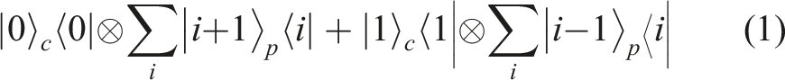
| 0 〉_{c} 〈 0 | \otimes \sum_{i} | i + 1 〉_{p} {〈 i | + | 1 〉}_{c} 〈 1 | \otimes \sum_{i} | i - 1 〉_{p} 〈 i |

(1)

The c and p subscripts refer to the coin and position registers. The positions are represented by integer states |n⟩ for $n \in Z$ .

The quantum walk model can be used in two different but related ways. Firstly, it can be used to model evolving beliefs or opinions, for example, subjective estimates of what a particular asset will be worth at a given future time. Different and even contradictory beliefs can be modeled in the quantum walk as a coherent superposition of different possible values. Secondly, it can be used to model actual asset prices, as observed in recorded transactions. A transaction behaves like a measurement on the quantum walk state, which forces the coherent superposition into a particular state. Some ways of inserting and tuning the level of decoherence are discussed by Orrell (2021), noting in particular that if the quantum walk is measured at every time increment, decoherence is complete and the quantum walk collapses to the classical version.

An interesting feature of long, coherent quantum walks is that the distributions become two-tailed, as do those of the quantum harmonic oscillator at higher energy levels (Orrell, 2020, Ch 10). Quantum dynamic models have been used to represent several cognitive scenarios (Busemeyer & Bruza, 2012, Ch 9), and oscillator models in particular have been used to model fluctuations in the stock market (Orrell, 2022). It is intriguing that the distributions produced by quantum walks with and without decoherence are similar to those produced by oscillator models at high and low energy levels.

This has provided considerable motivation for implementing quantum walk and oscillator models. However, experiments in simulating quantum walks and harmonic oscillators on real quantum computers have been very small so far, restricted to just 2 or 3 qubits, and have reported very noisy results using superconducting hardware (Kadian et al., 2021; Puengtambol et al., 2021; Qiang et al., 2016). The reasons for this are explained in the next section.

4. Quantum Counting and the Challenge of Recording Position

To simulate a quantum walk using repeated applications of the shift operator in equation (1), we need to model tossing a coin, and tracking position. The coin-toss is easy for today’s quantum computers to implement effectively. For example, we use a single qubit and a Hadamard gate which acts like a ‘beam-splitter’, putting the coin into a superposition of |0⟩ and |1⟩ states.

The bigger challenge for quantum computers today is tracking the position: in other words, the quantum counting problem (Haven et al., 2017, Ch 4). For non-negative numbers, the states |n⟩ can be associated with the energy levels in a harmonic oscillator (Jain et al., 2021). In theory this might connect the process of quantum counting with the use of motional modes in for quantum information processing, but this is not yet available on commercial quantum computers (Chen et al., 2021).

The most traditional way to represent numbers on a computer is to use some form of binary positional notation. For example, the binary expression 110 represents the number 6 (or the number 3, if the bits are read in reverse order). Quantum binary ‘adder circuits’ were designed by Feynman in the early papers that first motivated quantum mechanical computing (Feynman, 1986), but the ongoing presence of errors in NISQ-era machines limits the number of steps we can reliably count (Orts et al., 2020).

Choosing a binary positional encoding, as used in classical computing, makes quantum counting very susceptible to 2-qubit gate errors, because manipulating binary encodings takes a lot of entanglement and coordination between qubits. To compute the sum of two binary numbers A and B of bitlength n using classical Boolean algebra, we add (XOR) the least significant bits, and then at each other position we add the corresponding bits along with a ‘carry’ from the previous stage, setting the output and passing a ‘carry’ on to the next position. Feynman (1986) explained the quantum gate operations needed for each such step in the quantum full adder circuit of Figure 5, and modern versions are optimized variants on this theme (Orts et al., 2020). If it takes 11 2-qubit gates for each full-adder, then adding two single-byte (8-bit) numbers using this approach uses ∼80 2-qubit gates, so by the time such a register has successively added 10 numbers, the chances of an error are over 50% even with a two-qubit gate fidelity of 99.9%, which is on the high-end of performance estimates at the time of writing (IonQ Aria, 2022).

Figure 5.

A quantum full adder circuit, first introduced by Feynman (1986), uses 2 Toffoli and 3 CNOT gates, which is at least 11 2-qubit gates.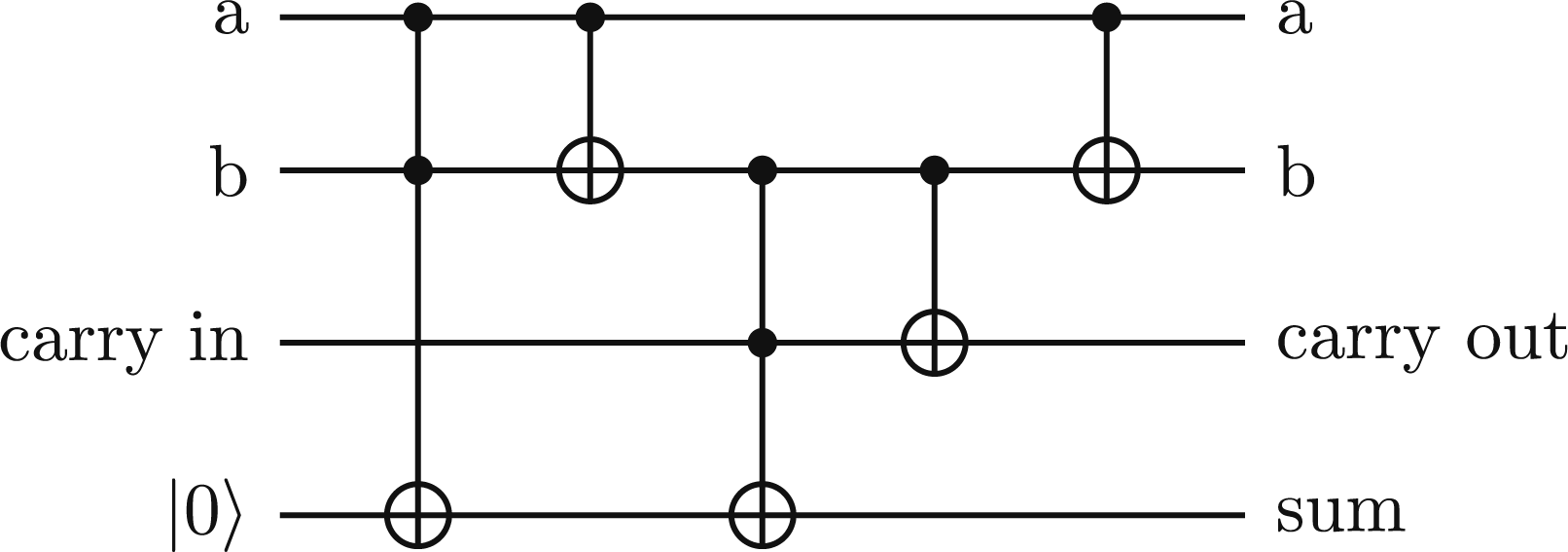

Error rates with quantum counting can thus undermine the simulation of quantum walks, and block this application of quantum finance. The problem is demonstrated in Figure 6, which compares quantum walks with ideal outcomes and with noise. This shows the vulnerability of the quantum counting process to noise after a handful of steps. It should be noted that some noise or decoherence can be useful in quantum models, for example, in deriving price estimates from many quantum walk simulations (Orrell, 2020, Ch 6). The predictions later in this paper are also averages over many somewhat-noisy circuits: the key engineering challenge here is to understand the noisy behaviors, and find those that work well enough to enable the task at hand.

Figure 6.

Ideal simulated quantum walk after 14 and 15 steps (left), compared with results simulated with expected noise (right). The ideal distribution has the two-tailed peaks characteristic of a quantum walk or harmonic oscillator, but this quickly gets lost with noise (right).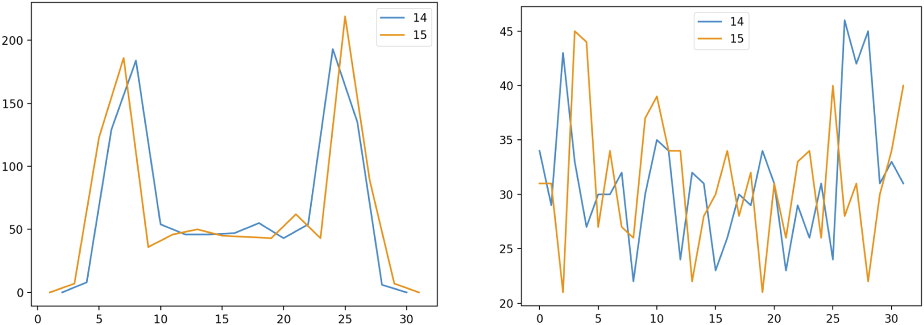

There are many optimizations and alternatives. We expect progress in quantum hardware to enable greater fidelity and stability, and eventually mid-circuit quantum error-correction should make the current problems with quantum counting obsolete — but this comes at the cost of waiting for fault-tolerant quantum computing. Quantum addition algorithms can be optimized (Cuccaro et al., 2004; Gidney, 2018), and the incremental operation of counting can be made simpler than repeated full-register addition (Li et al., 2014). An interesting benchmark challenge could be to design and evaluate quantum circuits and see how far they can count with $> 50 %$ fidelity, but that task is not undertaken here, because none of these methods simplify counting enough for many successive counting operations on nontrivial quantum registers to be performed accurately yet. Instead, this paper proposes alternative circuits that can be used to simulate steps and positions in a walk, without requiring exact counting.

5. Approximate Quantum Counting: Fault-Tolerant Circuits for Tracking Position

By now, the central modeling problem of this paper should be clear: we would like to be able to model a quantum walk on a quantum computer, but the use of positional binary notation to represent integer quantities requires ‘increment’ and ‘decrement’ operators that require too many entangling gates to give accurate results on current quantum hardware.

To avoid these pitfalls, we introduce alternative circuit designs that can also be used for recording position in a random walk. Instead of trying to ensure that every move goes up and down by exactly one step on the position axis, the position register is incremented using some gate combination that is likely to move the position by some amount that is generally positive for upward steps, and downwards for downward steps. Another way to describe this is that instead of putting all the randomness in the coin toss and following this with deterministic shift operators, we toss a random coin and then combine this with a somewhat-random shift operator. For larger circuits, such methods can give a walk that goes up and down more reliably than the results we get if we try to insist that the position represented by the state |n⟩ is an accumulation of exactly n steps of unit length in that direction.

The reader should note that all the results from the circuits in this section are statistical in nature, so the results are naturally noisy in various ways. Some of the randomness is purely quantum, in that different runs of the same circuit are expect to give different measurements according to the Born rule, and running jobs with more shots gives closer statistical approximations to the ‘real’ quantum distribution. For some of the design patterns in this section, randomness is also due to the way the circuits are constructed, so this randomness is expected and is classical in nature. Also, NISQ-era results also include noise from hardware errors. It is not always immediately obvious which sources of noise or randomness are most impactful for a given design, though some of the key features are noted.

5.1. Arc Counter Circuits

The Arc Counter circuit design uses only single-qubit rotations throughout. Such a representation is sometimes called a rotation encoding (Schuld & Petruccione, 2021). It is particularly easy to implement for a modest number of features, and can be incremented as new feature weights are encountered.

To use a rotation encoding for counting, qubits are rotated through particular arc-lengths or angles at each incremental step. Each qubit is used to represent one digit in a binary register, where each bit is twice as significant as its predecessor. At each step, each qubit traverses an arc that is inversely proportional to that qubit’s significance, as in Figure 7. This means that the n + 1^th qubit rotates at half the rate of the n^th qubit.

Figure 7.

Arc counter circuit.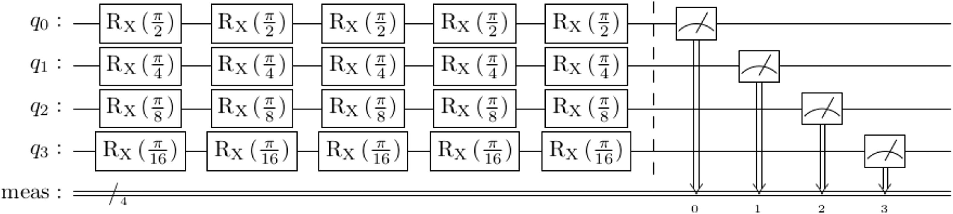

A good analogy for this representation is to think of each qubit as one of the hands on a traditional analog clock. On an analog clock, the minute hand cycles at 12 times the speed of the hour hand, and the second hand 60 times faster still, whereas in our binary clock, the ratio between the speed of rotation of each successive pair of ‘hands’ is 2:1. This analogy works well for the standard binary positional notation for integers, which can be thought of as a binary digital clock. In a digital register (or an abacus), the digits logically depend on one another for correct incrementing, because we need to know that one register is full before we increment the next. By contrast, the hour hand on a clock does not ‘carry’ information when the minute hand completes a cycle — it just rotates at its own slower pace. Thus the rotation encoding clock-based design requires much less coordination (and hence entanglement) between the qubits.

This comes at a representational cost — the register does not represent exact integers, and random variations in the outputs are expected, because many fractional angles are used throughout the circuit. (This is true for the basic counting operation, irrespective of whether the counting is coupled with a ‘coin toss’ operation).

Sample results from a quantum walk with an 8 qubit register are shown in Figure 8. Statistically noteworthy properties include:

• The mean distance from the starting point generally increases with the number of steps.

• In some cases, the position appears to jump ahead, because a high-order qubit is measured in the |1⟩ state. This can happen (with low probability) after just a single step.

• There are sometimes peaks in the distributions after specific powers of two or their combinations (e.g., peaks at 48, 64, 96). It may be possible and desirable to find ways to smooth out these peaks.

Figure 8.

Quantum walk results after different numbers of steps with arc counter circuit and an 8-qubit register. 1000 shots for each number of steps.

Since there are no 2-qubit entangling gates, error rates are lower, but there’s also no physical quantum advantage from this design — it is easy to model this distribution on a classical computer. It’s possible that such distributions might be useful models for random processes, but this would not require quantum computers to simulate.

5.2. Reversal and Superposition by Classical Post-Processing

An important feature of the traditional ‘binary adder’ circuit components is that they are able to decrement (subtract) as well as increment (add). The arc counter circuit, and the others below, do not support this feature. The logical work to guarantee that a change from 01111111 to 1000000 happens in-concert for all of the bits is precisely what we’ve given up, which makes it much harder to orchestrate a difference between positive and negative steps with large distances.

As noted by Haven et al. (2017, Ch 4), it is natural for quantum systems to have a lowest state which we may call |0⟩, and if we want to generate a full set of integers including the negative ones, these can be constructed as differences between positive natural numbers. This leads to an alternative method for simulating random walks that can evolve in both directions. We use two quantum circuits, one for the ‘up’ steps and one for the ‘down’ steps, and subtract the results from the down circuit from the results from the up circuit as a classical post-processing step. The ‘up’ and ‘down’ circuits can even be configured with different ‘clock speeds’, which has been done in the example of Figure 9.

Figure 9.

Two-directional arc walk circuit from combining positive and negative distributions. 1000 shots for each number of steps.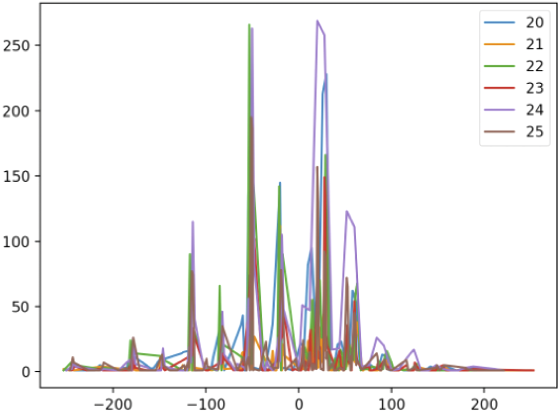

5.3. Arc Walk Counter Circuit

This circuit design combines the arc rotations of the Arc Counter design above, with the ‘Hadamard quantum coin’ prevalent in the quantum walk literature. At each step, a Hadamard gate ‘tosses a coin’, and if the outcome is ‘heads’, or |1⟩, a controlled rotation is performed on each of the other qubits, following the same pattern of angles as in the Arc Counter circuit above. This gives the circuit pattern of Figure 10.

Figure 10.

Arc walk counter circuit.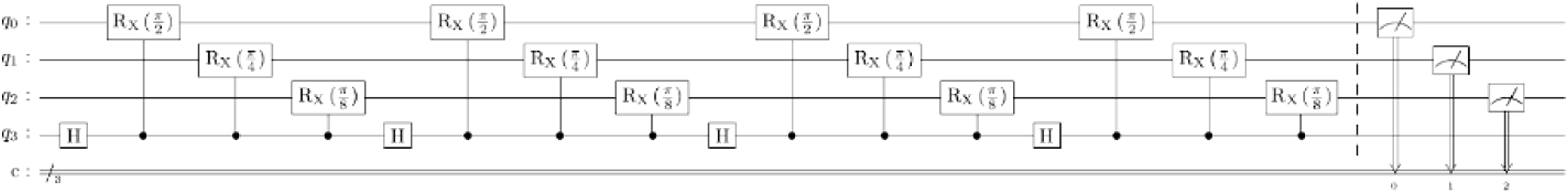

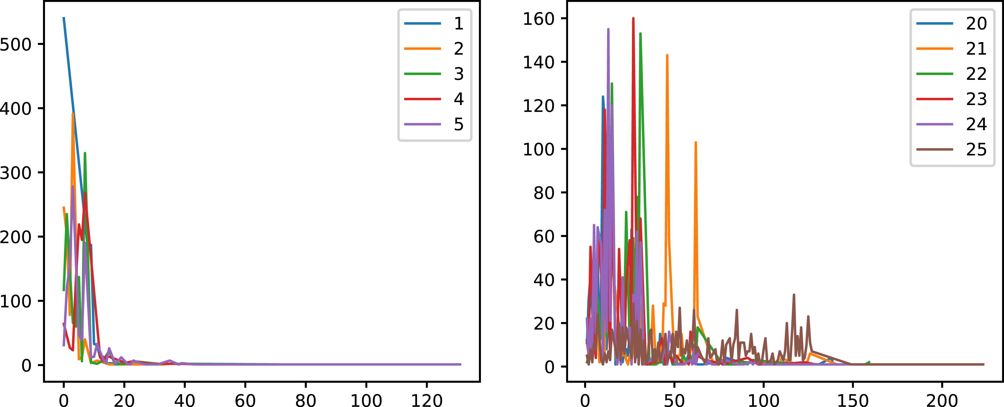
Example results (8 counter qubits, 10 to 15 steps) are shown in Figure 11. On the left is a purely incrementing circuit, on the right is a two-way walk using the reversal and superposition technique above.

Figure 11.

Example results for arc walk counter circuit (8 counter qubits, 10 to 15 steps). On the left is a purely incrementing circuit, on the right is a two-way walk using the reversal and superposition technique above. 1000 shots for each number of steps.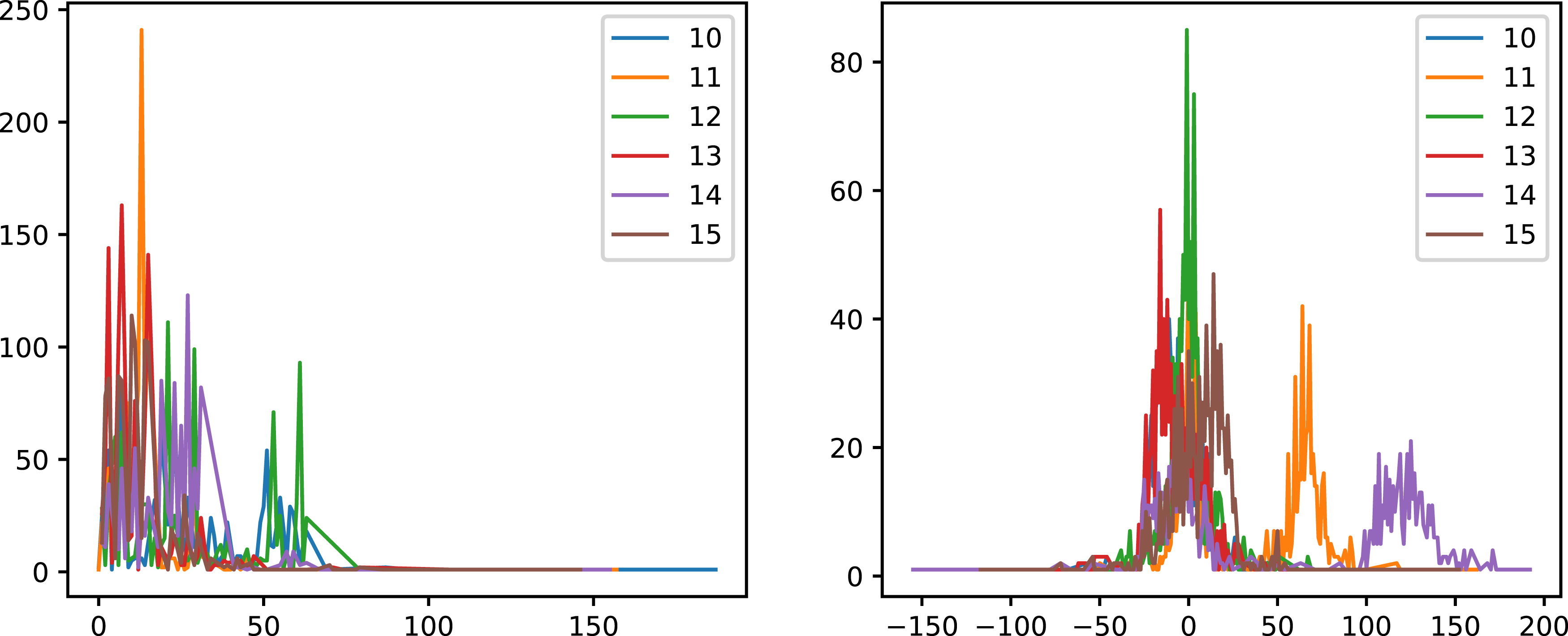

5.4. Random Jump Circuit

In this class of examples, instead of using smaller rotations for higher-order qubits, we set up the circuit so that these qubits are changed less often.

This can be done with and without a quantum coin controlling the gates. The example in Figure 12 uses a standard Hadamard quantum coin.

Figure 12.

Random jump circuit.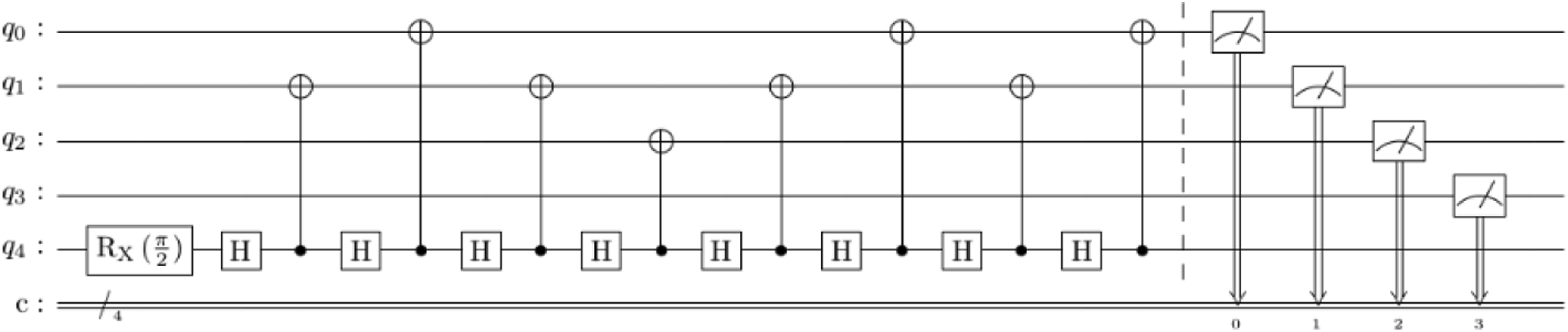

At each step, a different target qubit in the counter register is selected, according to some weighted random sampling function. This function should prefer the lower-order qubits). In the example below, the selection was done with the distribution {1/2, 1/4, 1/8, ….}. Note that the circuit creation now introduces classical randomness, as well as the circuit measurement still having quantum randomness.

Results for up to 9 steps, using an 8 qubit counter register, are shown in Figure 13. As expected, each walk can go both ways (because randomly flipping a bit can reduce as well as increase a number), though the average tendency for an individual walk is to increase. This is because the registers are initialized to zero, so the process randomly diffuses out from zero.

Figure 13.

Random jump circuit results (positive only on the left, two-way walk using reversal and superposition on the right). 30 random jump circuits per step, 30 shots per circuit.

5.5. Cascading Disjunction Circuits

‘Cascading disjunction’ is an extra circuit component that can be added to any of the counting circuits above. The idea uses a standard circuit component that performs Boolean disjunction, as in Figure 14.

Figure 14.

Boolean in-place disjunction circuit, which sets the state of the higher order qubit to the Boolean OR of the input states of the lower and higher order qubits. The X gates surrounding the Toffoli gate implement the usual NOT operations to turn an AND conjunction operator into an OR disjunction operator (A ∨ B = ¬(¬A ∧¬B)). Finally, the swap gate and the reset to |0⟩ operations ensure that the output is written back into the higher order qubit, and the ancilla qubit is reset to its initial state. Using this construction several times requires mid-circuit reset, so that the ancilla qubit can be reused.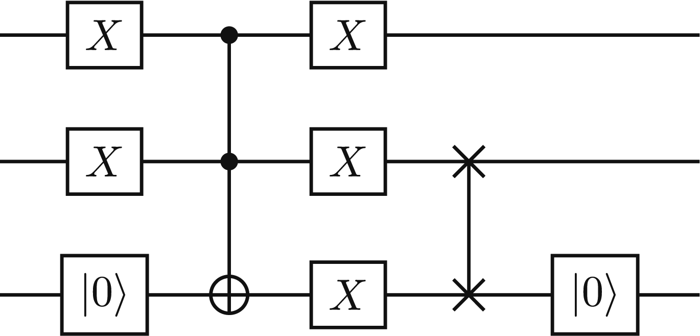

In this implementation, such gates are added between randomly chosen lower-and higher-order bits, using the same sampling distribution as in the Random Jump Circuits. This enables the values of lower-order qubits to propagate to higher-order qubits, which increases and tends to preserve progress in the walk, because the higher-order qubits are less likely to be randomly selected to be switched back to |0⟩ later.

Results of including this technique are shown in Figure 15 (positive only on the left, two-way walk using reversal and superposition on the right). The walks are still random, but propagating more reliably with the cascading disjunction components.

Figure 15.

Cascading disjunction circuit results (positive only on the left, two-way walk using reversal and superposition on the right). 30 random jump circuits with cascading disjunctions per step, 30 shots per circuit.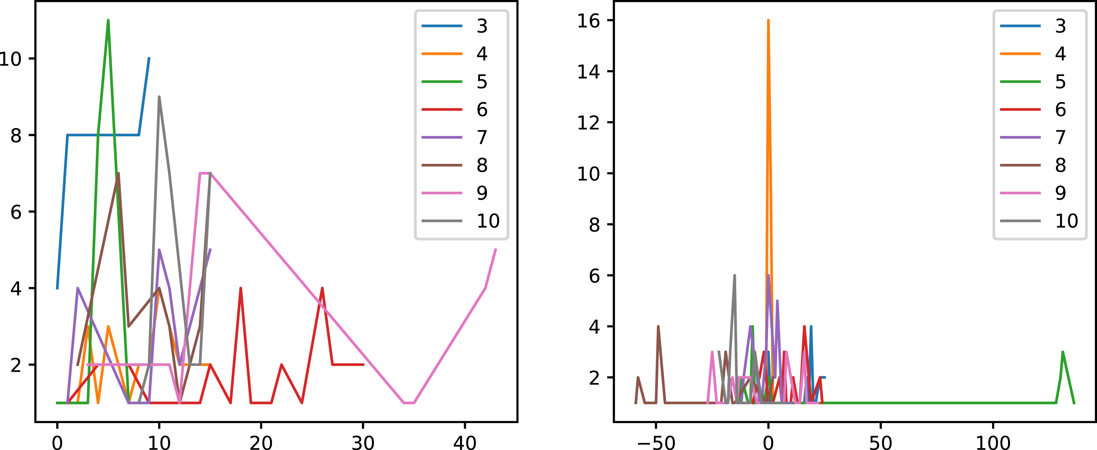

Another variant of this technique would be to add a conjunction between the coin qubit and the target qubit, that sets the next higher qubit to |1⟩ before reversing the target qubit to |0⟩. This would behave like a limited-carry operation: it performs some of the coordination between qubit values in the traditional bit-counter circuits in the literature, but much less, in a much more targeted fashion.

6. Preliminary Results of Counting Circuits, With and Without Noise

The big advantage for the simpler models presented here is that we can run them much more accurately (and quickly) on NISQ-era quantum hardware. Preliminary results for the different circuit designs presented in this paper are given in Tables 1 and 2. The goal of the new circuits is more reliable representation and incrementing of position, so the key comparison is with a binary counter itself, rather than the use of a binary counter going up and down in a random walk. The new methods are evaluated just with n positive steps, without subtracting the results of a walk in the other direction. The use of cascading disjunctions is included in the ideal ‘random jump’ circuit, though not in the noisy simulation, because the support for mid-circuit reset on the ancilla qubit is not guaranteed today. The simulations used 6-qubit counting registers, so can represent numbers from 0 to 63.

Table 1.

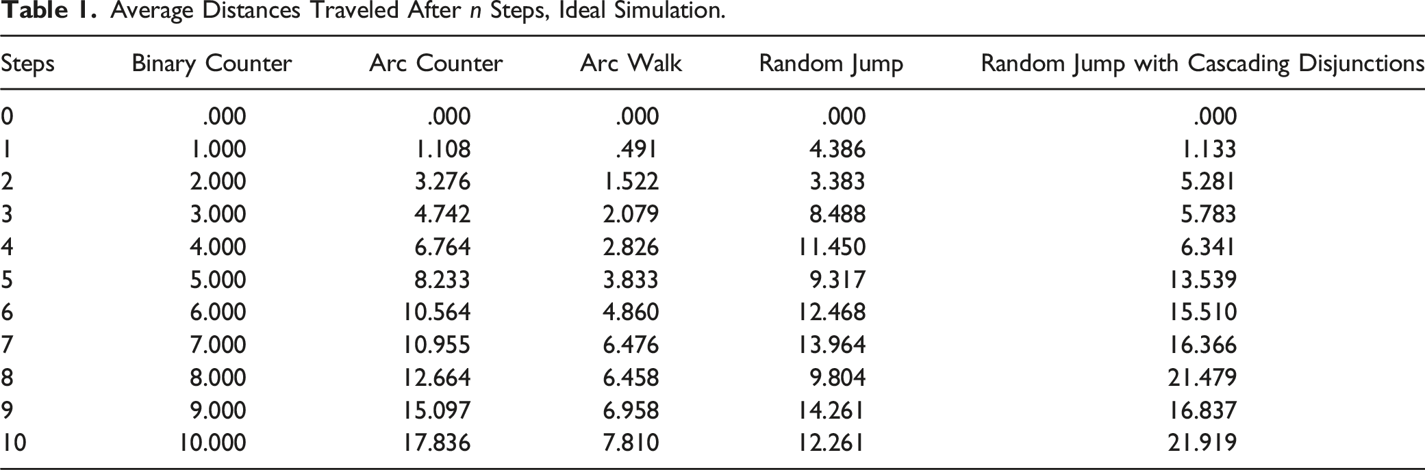
Average Distances Traveled After n Steps, Ideal Simulation.

Steps	Binary Counter	Arc Counter	Arc Walk	Random Jump	Random Jump with Cascading Disjunctions
0	.000	.000	.000	.000	.000
1	1.000	1.108	.491	4.386	1.133
2	2.000	3.276	1.522	3.383	5.281
3	3.000	4.742	2.079	8.488	5.783
4	4.000	6.764	2.826	11.450	6.341
5	5.000	8.233	3.833	9.317	13.539
6	6.000	10.564	4.860	12.468	15.510
7	7.000	10.955	6.476	13.964	16.366
8	8.000	12.664	6.458	9.804	21.479
9	9.000	15.097	6.958	14.261	16.837
10	10.000	17.836	7.810	12.261	21.919

Table 2.

Average Distances Traveled After n Steps, Noisy Simulation and QPU.

Steps	Binary Counter	Binary Counter (QPU)	Arc Counter	Arc Counter (QPU)	Arc Walk	Random Jump
0	.000	.00	.000	.002	.000	.000
1	15.606	21.946	1.312	1.94	2.562	1.742
2	25.123	32.771	3.461	4.412	3.859	2.618
3	30.504	32.802	5.488	5.782	6.223	5.919
4	29.921	33.603	6.824	6.236	8.721	9.279
5	31.046	32.212	8.931	10.208	10.773	10.250
6	31.732	33.317	10.442	12.984	12.627	10.981
7	30.837	32.978	11.183	12.389	14.978	12.401
8	31.894	33.775	13.148	13.682	15.898	14.568
9	30.99	32.989	14.614	15.504	17.300	12.684
10	31.912	34.101	18.459	19.666	20.907	17.216

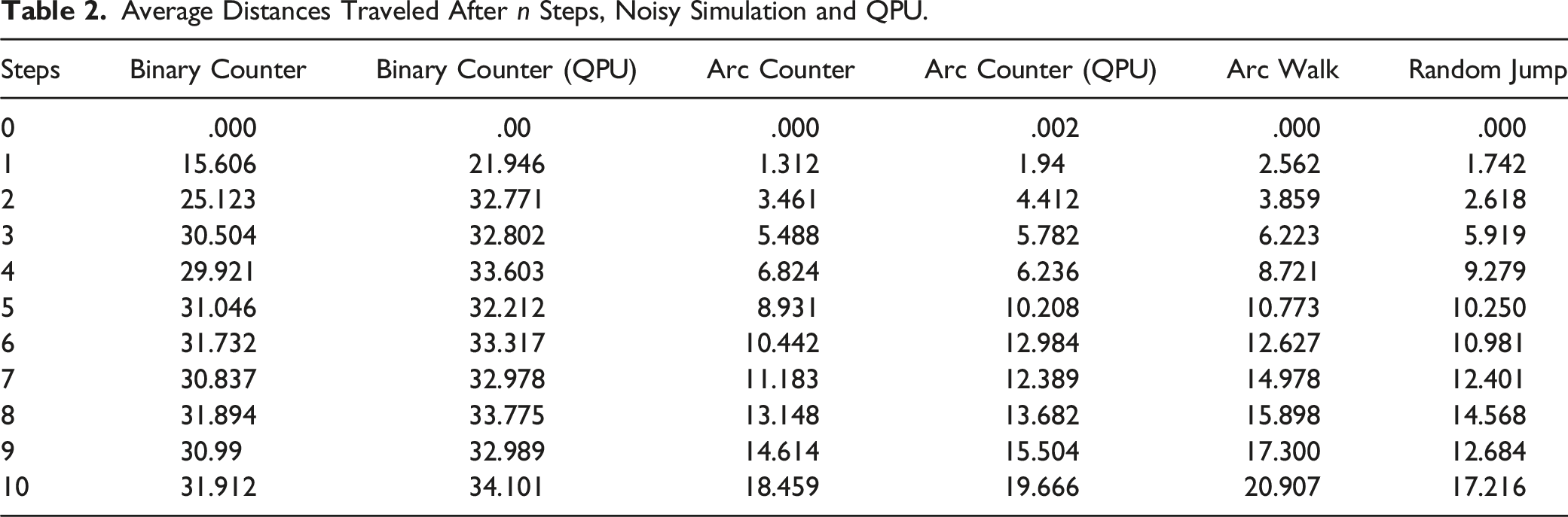
Ideal simulations can only be performed for small numbers of qubits (as a rule-of-thumb, as we pass 30 qubits we start to break the limits of classical simulation). In addition, the binary counter and arc counter circuits were run on a quantum computer with 11 trapped-ion qubits, described by Wright et al. (2019). These results are also show in Table 2, with the label QPU (quantum processing unit). Note that 11 qubits is relatively small by today’s standards: the number of reliable qubits in state-of-the-art machines in 2023 is at least in the 20s (IonQ Aria, 2022). The older machine was deliberately chosen for this experiment, because it highlights the frailty of exact binary counting circuits compared with approximation counting circuits.

The random jump results were computed using 30 shots on each of 30 randomly-generated circuits, so these results include both classical and quantum randomness. The binary and arc circuits are generated deterministically, so these results include 1000 shots for a single circuit, and all the randomness is quantum.

Key findings include:

• The binary counter results are perfect with ideal simulation, but are rendered useless in the noisy simulation. They quickly converge to a random number around 32, which is the average

• For all the other circuits, the difference between ideal and noisy results is much less.

• The average results for the arc counter and arc walk circuits are the most reliable for simulating a monotonically-increasing position, with or without noise.

• The random jump results also tend to increase, but tend to plateau and then move up and down randomly. (This randomness is smaller with a larger register).

The QPU results for binary and arc counting are compared graphically in Figure 16. This shows how quickly the binary counter becomes useless on a real QPU, whereas by contrast, the arc counter QPU results stay close to the ideal simulated results.

Figure 16.

Ideal and actual QPU results for binary counter and arc walk circuits. The QPU are much closer to the ideal monotonically-increasing results for the arc counter, whereas they are useless after 2 steps for the binary counter.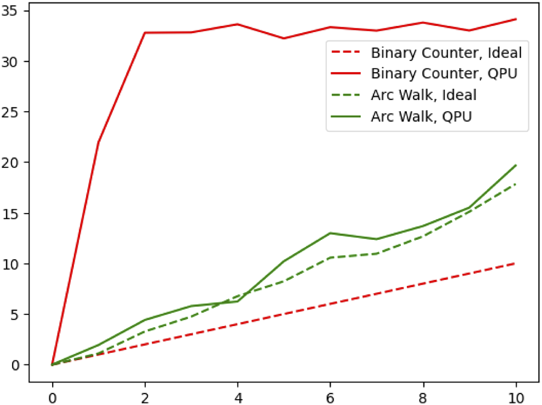

6.1. Quantum Walk Distributions and Real Financial Data

The notion that market returns follow a normal (or log-normal) distribution is standard and established in quantitative finance, even though it has been known for decades that heavy-tailed distributions are sometimes a better fit (Mandelbrot, 1963; Zi-Yi, 2017). In the traditional random walk model, daily changes in asset price are also assumed to follow a normal distribution, or even more simply, to take a constant step in either direction, and the accumulation of many such steps in a binomial distribution eventually approximates the normal distribution.

In practice, daily relative changes in stock prices also tend to have a distribution where most values cluster around zero, but significant outliers cause a normal distribution fitted with the same mean and standard deviation to underestimate the density in the middle if the distribution. This is shown for the Dow Jones Industrial Average in Figure 17 (using data from the Yahoo! Finance API). An initial comparison shows that distributions of daily changes generated by the arc walk and random jump circuits also follow this heavy-tailed pattern, which is not modeled well by normal approximations.

Figure 17.

Distributions of relative changes in the Dow Jones Industrial Average, and in quantum approximate counting simulations. The dashed curve (red) shows the best-fit normal distribution, that is, the normal with the same mean and variance.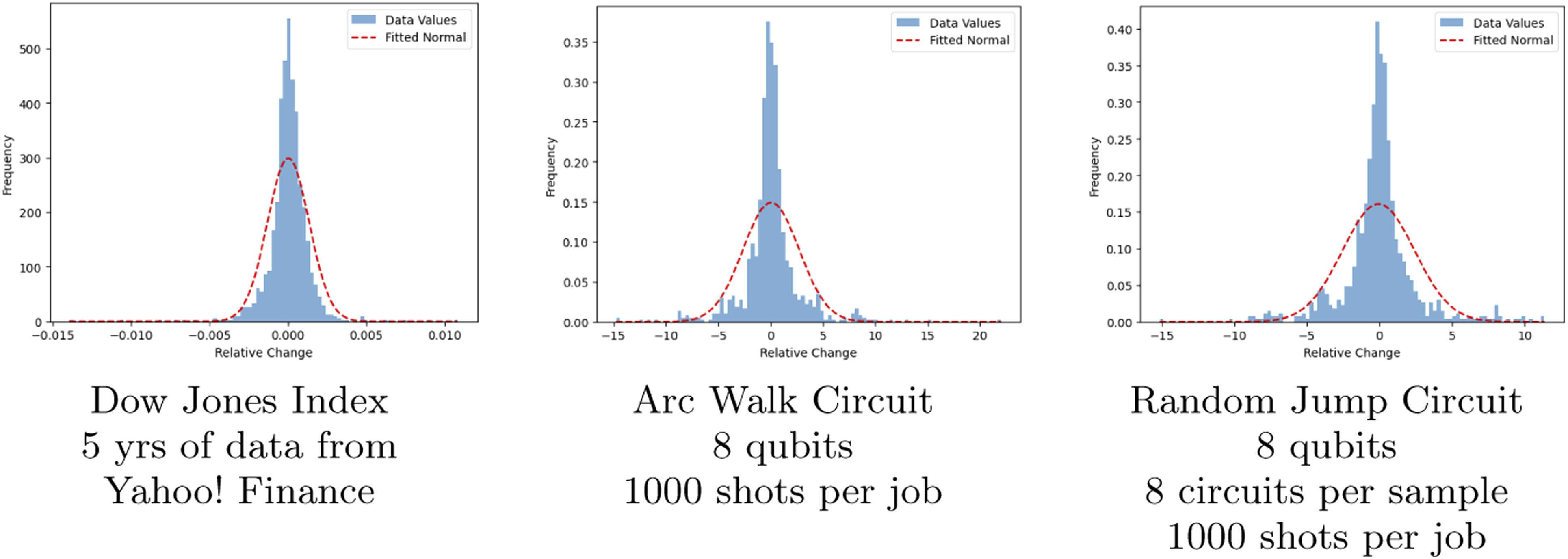

This does not show that the quantum approximate counting circuits give a better prediction of stock price changes on a specific day. But it does show that the distribution of possible changes can be better-adapted to real-world financial data, without the artificial constraint that daily changes should be normally or uniformly distributed.

It should be noted that quantum results in Figure 17 are obtained with some parametrization and averaging, because all quantum job results are averaged over the number of shots, and the random jump circuits are averaged over a number of sample circuits as well. The impact of long-tail measurements depends on how large a sample we take. While this implies that there is some arbitrariness in results, it also means that parameters such as the number of qubits, circuits, and shots can be tuned to model particular datasets.

In related work, IonQ quantum computers have also been used to model the normal distribution itself, using a matrix product state technique that can readily be adapted to other distributions, because it relies on piecewise polynomial approximation (Iaconis et al., 2023). One of the longer-term promises of such work is that such distributions can be used as inputs for models such as the Monte Carlo simulations advocated by Egger et al. (2020). If we have a reliable circuit for preparing a particular distribution, then such a circuit could be used as input for Monte Carlo modeling by entangling its output with the simulated variables, rather than by sampling an individual number from the distribution and using this as a single ‘classical’ random input value.

7. Quantum Walks with Mid-Measurement: A Quantum Zeno Effect

A crucial difference between classical random walks and quantum walks is that quantum walks behave differently depending on when they are measured. There is no classical counterpart for this behavior, because a hallmark of classical systems is that their state is revealed but not changed by measurement.

In theory, it is possible to prevent a quantum system from changing state at all, by measuring smaller and smaller intervals. As a simplest example, the gate R_X(θ) from Figure 1 operating on a qubit in state |0⟩ produces the state

R_{X} (2 θ) (| 0 〉) = \cos (θ) | 0 〉 + i \sin (θ) | 1 〉

The probability of transitioning to the state |1⟩ is thus proportional to sin²(θ) which tends to zero for small θ, and it is easy to see that if a larger angle is divided into smaller and smaller increments, the probability of observing a transition to the state |1⟩ in any of these increments also tends to zero, because lim_n→∞(n) sin²n → 0.

This phenomenon is sometimes called the quantum Zeno effect, after Zeno’s classical paradox of motion. Of crucial interest for this paper, such effects have also been observed in psychology. Kvam et al. (2015) demonstrated that participants are likely to form less extreme judgments of moving scenes if asked to judge the motion in smaller time-frames, and Yearsley and Pothos (2016) demonstrated that participants evaluating evidence in a criminal trial are more likely to change their minds if several pieces of evidence are presented before asking for a decision.

It is easy to add mid-circuit measurement to our quantum approximate counting circuits and to evaluate the results, at least in simulation. (The availability of mid-circuit measurement varies across quantum platforms currently, partly because the accuracy of the measurement and reset operations is hard to guarantee.) Example results are shown in Figure 18, simulating walks with 20 steps, with no mid-measurement, measurement every 7 steps, and measurement every step. The average positions reached by these walks were 35.6, 14.3, and 5.7 respectively, so as expected, the use of mid-measurement reduces the average distance traveled in the quantum walk. (It is not always this simple, particularly due to periodicity.) A further step for this research would be to experiment with parameters including the number of steps, distribution of step sizes, and frequency of measurements, to see if different levels of deliberate decoherence can bring the quantum results of Figure 18 closer to the distributions observed with the Dow Jones Index and other asset prices.

Figure 18.

Arc counter circuit results, simulating the results of quantum walks with 20 steps, with and without mid-circuit measurement at the given positions.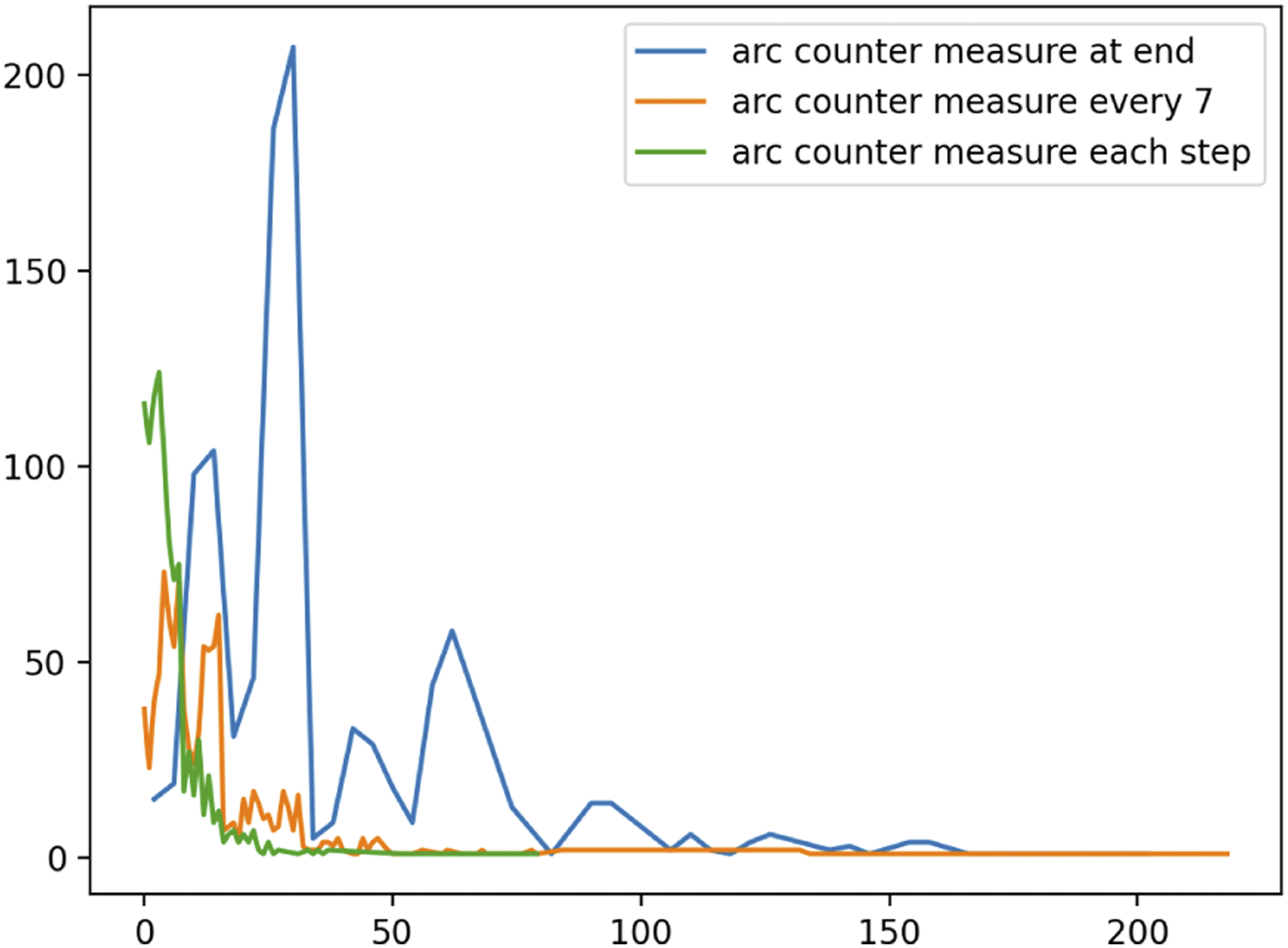

7.1. Mid-Measurement, Transactions, and the Housing Market

In the quantum economics theory of Orrell (2020), the act of measurement is compared with fixing a transaction, and subjective opinions of value can vary like quantum states between transactions. By analogy with the quantum Zeno effect, we may expect that opinions about prices vary less if there are more frequent measurements, i.e. more frequent transactions. Evidence is presented by Orrell (2022) and Orrell and Richards (2023) showing that price volatility is not constant, and that high volatility corresponds to both uncertainty in value, and wide ranges between different bid prices and asking prices. This section presents some findings from housing market data, indicating that indeed, larger transaction volumes correlate with smaller differences between the higher prices asked by sellers, and lower prices offered by buyers.

The range of prices offered to buy or sell an item is typically much more apparent in the housing market than the stock market, because each item for sale is priced and negotiated much more individually. A standard process involves the use of comparable sales or comps, in which transactions on properties nearby in time, space, and value are used to form a pricing estimate (Pagourtzi et al., 2003). If these nearby transactions correspond to measurements of the system, then the quantum Zeno effect would suggest that the outcome of this measurement is more certain if there are more nearby transactions.

This effect was demonstrated in practice using the following modeling assumptions, and summary data published by Zillow.

When a house sells for less than its original listing price, we assume that this indicates a difference between the seller’s and the buyer’s estimate of the house’s value. Larger uncertainties in the market would support larger differences of opinion. Even when considering monthly averages of data, we would expect that a smaller number of sales in a given area would contribute to greater market uncertainty, and this should correlate with a greater difference between the list price and the sale price.

By contrast, when a house sells for more than its original listing price, we assume that there are other factors involved: in particular, this situation is common when there are other bids on the property from other potential buyers, so a minimum value is already established without the need for previous comparable transactions.

Thus, we assume that the markets where lack of comparables is a primary factor in price uncertainty are those where the average sale price is less than the average list price. It follows that, if we restrict our attention to markets where the average sale price is less than the average list price, we should see evidence that lower transaction volumes are correlated with greater disparities between list price and sale price.

Data used to test these hypotheses was gathered from the Zillow Housing Data portal¹. The datasets are summary statistics: counts and averages. These are only comparable within a given metro area: for example, 2000 sales in a month would be very low for New York, NY, and very high for Wichita, KS. Thus we compute correlations by comparing monthly statistics within each metro area.

The algorithmic steps are as follows:

• For each metro area:

• For each month:

– Collect the sales count and the average list-to-sale price ratio.

– If the average list-to-sale price ratio is greater than 1, skip this month.

• This gives a set of (count, ratio) pairs, e.g. [(822, .98), (785, .96), (803, .97)], etc.

• Compute the Pearson correlation coefficient between these sales counts and list-to-sale price ratios.

• Gather the Pearson correlation coefficients into a histogram to see if there is a general trend.

The result is in Figure 19. Nearly all the correlations are strongly positive. This shows that, in cases where a house is sold for less than its asking price, there is a very strong correlation between the translation volume, and the closeness of the list and the sale prices.

Figure 19.

Histogram showing correlations between larger numbers of transactions and smaller list-to-sale price differences. Data from Zillow Housing Data.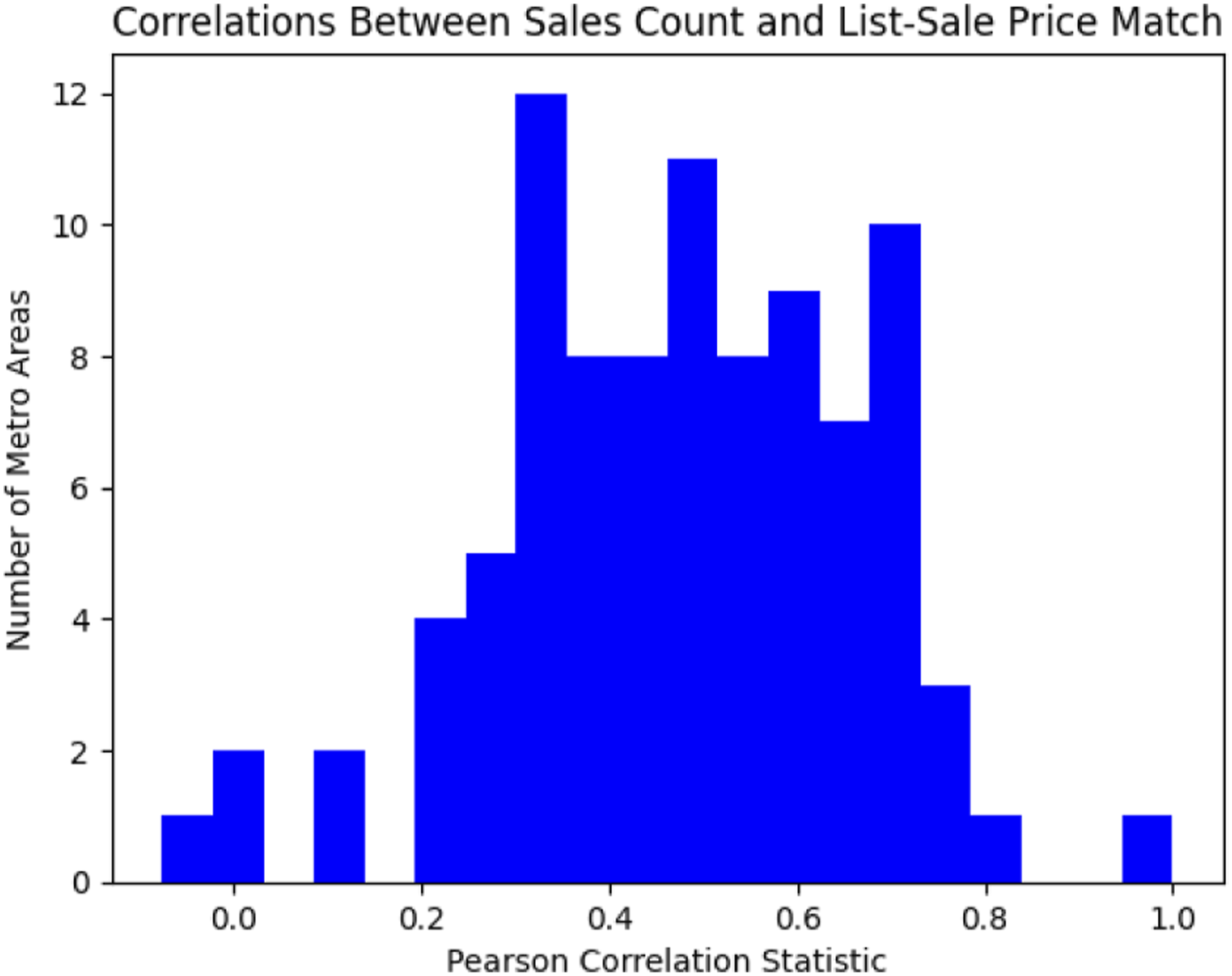

In addition to the number of sales in a region, it is instructive to look at the correlation between home prices and the list-to-sale price ratio since the price of a home is the driving factor in a home purchase. As a proxy for home prices we use the Zillow Home Value Index (ZHVI) which reflects the typical value for homes in the 35th to 65th percentile range.

Figure 20 shows both the raw monthly values (above) for the San Francisco region as well as monthly changes (below) comparing the ZHVI and list-to-sale ratio values for the last 6 years. The bottom chart shows more clearly the positive correlation between the two if we consider monthly changes. Monthly changes give a better sense of market ups and downs. As prices fall, we see that buyers are more likely to bid lower than the list price. Conversely, in a rising market, buyers are more likely to bid more than the list price.

Figure 20.

Monthly values of Zillow Home Value Index (ZHVI) and list-to-sale ratio as well as monthly changes that show positive correlation in both rising and falling markets.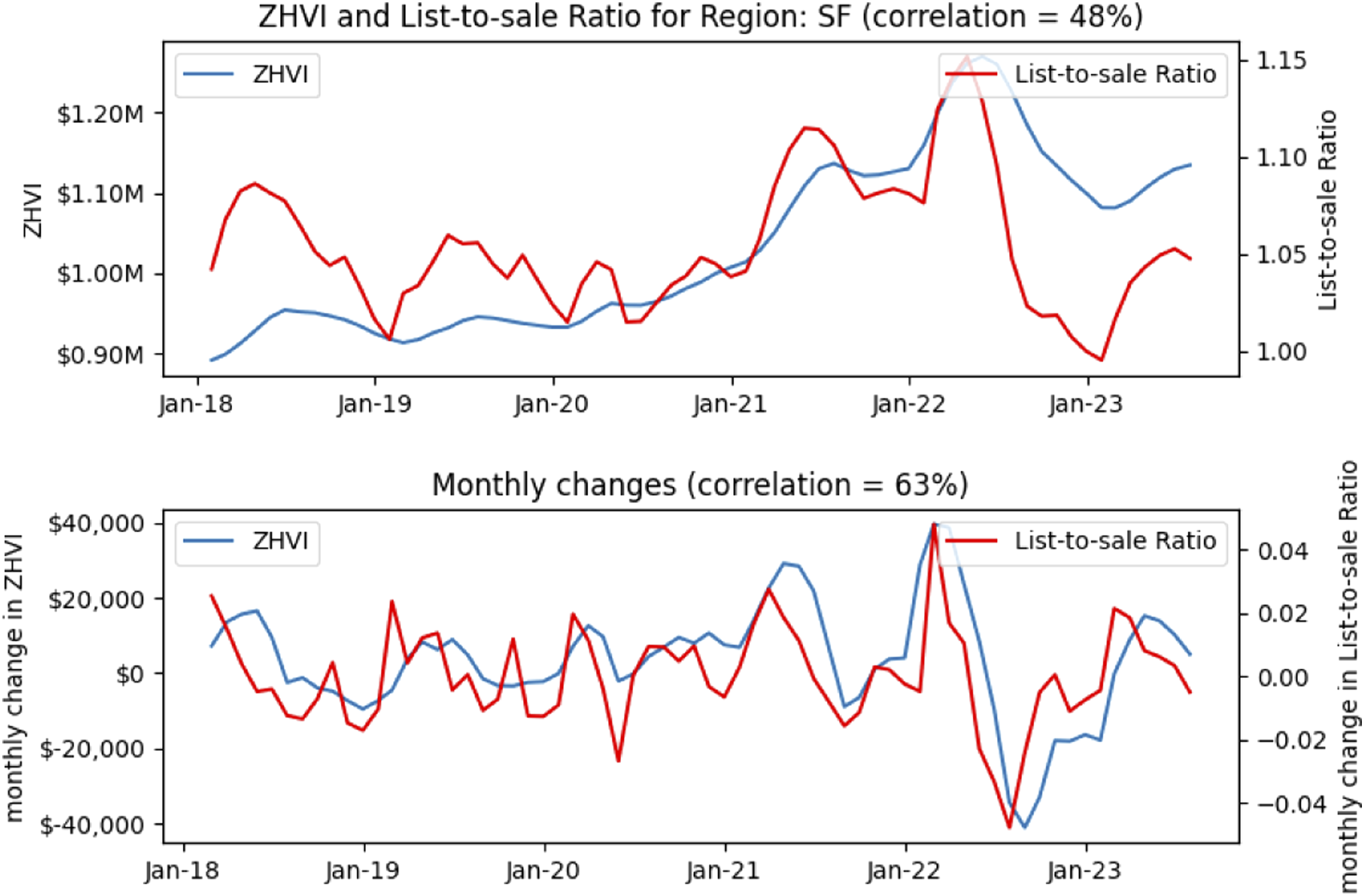

That fewer transactions correlates with larger list-to-sale price ratios is in line with the trends expected from quantum economics models, in which various beliefs and opinions about value can evolve and diverge more when there are fewer transactions or measurements. The correspondence between overall price changes and list-to-sale ratios could be described by a quantum walk with a clear directional momentum. However, it is also easy to propose simple non-quantum models for these behaviors. Fewer comparable samples leads to greater sampling error and thus greater price uncertainty: thus lower liquidity brings higher volatility. One potential strategy for evaluating and distinguishing which approaches are better would be to consider the dynamics/evolution of prices in such models: for example, to try applying the quantum Monte Carlo sampling reduction described by Egger et al. (2020) to the problem of making accurate price estimates with fewer comparable sales.

7.2 Macro Effects: Collective Beliefs and Reckonings

As well as the belief states of individuals, quantum models have been proposed to represent the beliefs and ideologies of whole groups of people (Kitto & Widdows, 2016). With pricing models, the influence of contrasting beliefs held by groups of people is especially important — as Bachelier (1900) wrote, “Contradictory opinions in regard to these fluctuations are so divided that at the same instant buyers believe the market is rising and sellers that it is falling.” The importance of group beliefs is particularly apparent with rare luxury goods: the opinion of a few wealthy people can be enough to establish high prices for rare art, even without mass appeal.

In such a model, decision making becomes partly a constructive process. This is standard in quantum models for individual behavior, where participants tend to remain in a particular state once it has been chosen if an identical question is asked (Busemeyer & Bruza, 2012). Memory and recollective processes are studied from a quantum-like point of view by Waddup et al. (2023), who try to measure the influence of intervening steps in decision-making. One problem in demonstrating quantum-like properties, such as violations of temporal Bell inequalities, in these processes is that it is hard to rule out interference and signaling.

With financial decisions, ‘signaling’ is a clear part of making decisions collective. Historic examples are notable in the early telegraph era, where the ability to publish outcomes of horse-races and stock-transactions across large distances led to opportunities for short-term fraud and long-term financial services industries (Standage, 1998). Applying the notion of quantum measurement and state collapse to a whole group of people may sound far-fetched in the abstract, but less so when we consider how much modern infrastructure is built to make a decision in one place felt immediately everywhere. More generally, there are many social processes where the views of groups of people are changed, sometimes reluctantly, in the face of events — here the notion of a ‘transaction’ becomes the even more general ‘reckoning’.

Such collectively-recognized events are naturally scarce: we cannot create housing transaction examples in the same way that we can collect and annotate training examples with other supervised machine learning models. Any quantum ‘modeling advantage’ with such problems would be especially compelling, because when training data is scarce, we cannot just train larger classical models for longer and assume they will give better results. Quantum Monte Carlo pricing models are expected to converge faster with fewer samples (Rebentrost et al., 2018), which raises the intriguing question of whether such techniques lead to faster convergence with fewer examples from real experience. Even with other asset types such as stocks and options where transaction samples are plentiful and speed is more important, the dynamic effects of large events from other market sectors could be anticipated more effectively. There is still scope for the use of quantum-like models in these areas, even before the widespread use of quantum computers.

8. Conclusions and Future Work

This paper has introduced and explored quantum approximate counting circuits, as fault-tolerant alternatives to the traditional quantum walk design, particularly for the way position is tracked and incremented. The new designs presented here lack some of the mathematical elegance, and the theoretical results, that accompany the traditional quantum walk design: and in particular, there are no longer unit increment and decrement operators that correspond to the ladder operators of a quantum oscillator. However, the enormous advantage for the simpler models presented here is that they behave much more accurately on NISQ-era quantum hardware, which could contribute to commercially advantageous applications of quantum computers in economics.

These are just prototype designs so far. The main next steps for this work are to evaluate the proposals more quantitatively, answering the following two questions:

1. How do results on NISQ-era quantum computers correspond to ideal or simulated results for small circuits, and what does this indicate about the expected behavior on quantum hardware for systems that are too big to simulate on classical hardware?

2. How do results compare with the distributions observed with real market behaviors?

The ideal outcome of this research is that we would find circuit walk designs that are robust enough to given better models of market behavior that include some of the benefits of quantum approaches noted by Orrell (2020), while being able to run on today’s quantum hardware without waiting for error-correction.

Given the crucial and explicit role that measurement plays in quantum models, it is possible that some of the earliest such quantum advantages will be apparent in markets where a small number of significant transactions can dramatically influence the price of a particular asset. An initial analysis suggests that the housing market may be an appropriate area to test this hypothesis.

This work can be seen as part of a larger program to bring value in economic modeling on quantum computers. Other successes for quantum circuit designs include modeling and sampling from key distributions (Iaconis et al., 2023), and demonstrating particularly effective time-series models using copula functions implemented using entanglement (Zhu, Shen, et al., 2022). Related work in cognitive science has demonstrated that simple quantum circuits can also be used to model decision-making processes (Widdows & Rani, 2022). In the next few years, it is likely that several such small components, being developed today, will be used as key building blocks in the first profitable applications of quantum computing in economics.

Footnotes

Acknowledgements

The author would like to thank Emmanuel Pothos and David Orrell for interesting conversations and encouragement.

Declaration of Conflicting Interests

The author(s) declared no potential conflicts of interest with respect to the research, authorship, and/or publication of this article.

Funding

The author(s) disclosed receipt of the following financial support for the research, authorship, and/or publication of this article: This work was funded by IonQ, Inc.

ORCID iD

Dominic Widdows

Note

References

Aharonov

Davidovich

Zagury

(1993). Quantum random walks. Physical Review A, 48(2), 1687–1690.

Bachelier

(1900). Théorie de la spéculation. Annales Scientifiques de l’Ecole Normale Superieure, 17, 21–86.

Busemeyer

J. R.

Bruza

P. D.

(2012). Quantum models of cognition and decision. Cambridge University Press.

Cady

(2015). What is math? CreateSpace independent publishing platform.

Chen

Gan

Zhang

J. N.

Matuskevich

Kim

(2021). Quantum computation and simulation with vibrational modes of trapped ions. Chinese Physics B, 30(6), 060311. https://doi.org/10.1088/1674-1056/ac01e3

Cuccaro

S. A.

Draper

T. G.

Kutin

S. A.

Moulton

D. P.

(2004). A new quantum ripple-carry addition circuit. arXiv preprint quant-ph/0410184 .

Egger

D. J.

Gambella

Marecek

McFaddin

Mevissen

Raymond

Simonetto

Woerner

Yndurain

(2020). Quantum computing for finance: State-of-the-art and future prospects. IEEE Transactions on Quantum Engineering, 1, 1–24. https://doi.org/10.1109/TQE.2020.3030314

Feynman

R. P.

(1986). Quantum mechanical computers. Foundations of Physics, 16(6), 507–532.

Gidney

(2018). Halving the cost of quantum addition. Quantum, 2, 74. https://doi.org/10.22331/q-2018-06-18-74

10.

Haven

Khrennikov

A. Y.

Robinson

T. R.

(2017). Quantum methods in social science: A first course. World Scientific Publishing Company.

11.

Iaconis

Johri

Zhu

E. Y.

(2023). Quantum state preparation of normal distributions using matrix product states. arXiv preprint arXiv:2303.01562 .

12.

IonQ Aria . (2022). IonQ Aria furthers lead as world’s most powerful quantum computer. https://ionq.com/news/february-23-2022-ionq-aria-furthers-lead (Accessed 28 May, 2022).

13.

Jain

V. K.

Behera

B. K.

Panigrahi

P. K.

(2021). Quantum simulation of discretized harmonic oscillator. Quantum Studies: Mathematics and Foundations, 8, 375–390. https://doi.org/10.1007/s40509-021-00250-0

14.

Kadian

Garhwal

Kumar

(2021). Quantum walk and its application domains: A systematic review. Computer Science Review, 41, 100419. https://doi.org/10.1016/j.cosrev.2021.100419

15.

Kitto

Widdows

(2016). Ideologies and their points of view. In Quantum interaction: 9th International Conference, QI 2015, Filzbach, Switzerland, July 15-17, 2015, Revised selected papers 9 (pp. 216–227). Springer.

16.

Kvam

P. D.

Pleskac

T. J.

Busemeyer

J. R.

(2015). Interference effects of choice on confidence: Quantum characteristics of evidence accumulation. Proceedings of the National Academy of Sciences, 112(34), 10645–10650. https://doi.org/10.1073/pnas.1500688112

17.

Yang

Torres

C. M.

Jr Zheng

Wang

K. L.

(2014). A class of efficient quantum incrementer gates for quantum circuit synthesis. International Journal of Modern Physics B, 28(01), 1350191. https://doi.org/10.1142/S0217979213501919

18.

Mandelbrot

(1963). New methods in statistical economics. Journal of Political Economy, 71(5), 421–440.

19.

Nielsen

M. A.

Chuang

(2002). Quantum computation and quantum information. Cambridge University Press Edition, 2016: American Association of Physics Teachers.

20.

Orrell

(2020). Quantum economics and finance: An applied mathematics introduction. Panda Ohana Publishing.

21.

Orrell

(2021). A quantum walk model of financial options. Wilmott, 2021(112), 62–69. https://doi.org/10.1002/wilm.10918

22.

Orrell

(2022). A quantum oscillator model of stock markets. Available at SSRN 3941518 .

23.

Orrell

Richards

(2023). Keep on smiling: Market imbalance, option pricing, and the volatility smile. Wilmott, 124, 58–64. https://doi.org/10.54946/wilm.11108

24.

Orts

Ortega

Combarro

E. F.

Garzón

E. M.

(2020). A review on reversible quantum adders. Journal of Network and Computer Applications, 170, 102810. https://doi.org/10.1016/j.jnca.2020.102810

25.

Pagourtzi

Assimakopoulos

Hatzichristos

French

(2003). Real estate appraisal: A review of valuation methods. Journal of Property Investment & Finance, 21(4), 383–401. https://doi.org/10.1108/14635780310483656

26.

Puengtambol

Prechaprapranwong

Taetragool

(2021). Implementation of quantum random walk on a real quantum computer. In Journal of physics: Conference series (Vol. 1719, p. 012103). IOP Publishing.

27.

Qiang

Loke

Montanaro

Aungskunsiri

Zhou

O’Brien

J. L.

Wang

J. B.

Matthews

J. C.

(2016). Efficient quantum walk on a quantum processor. Nature Communications, 7(1), 11511. https://doi.org/10.48550/arXiv.1510.08657

28.

Rebentrost

Gupt

Bromley

T. R.

(2018). Quantum computational finance: Monte Carlo pricing of financial derivatives. Physical Review A, 98(2), 022321. https://doi.org/10.1103/PhysRevA.98.022321

29.

Scholes

Black

(1973). The pricing of options and corporate liabilities. Journal of Political Economy, 81(3), 637–654.

30.

Schuld

Petruccione

(2021). Machine learning with quantum computers. Springer.

31.

Stamatopoulos

Egger

D. J.

Sun

Zoufal

Iten

Shen

Woerner

(2020). Option pricing using quantum computers. Quantum, 4, 291. https://doi.org/10.48550/arXiv.1905.02666

32.

Standage

(1998). The Victorian internet: The remarkable story of the telegraph and the nineteenth century’s online pioneers. Phoenix London.

33.

Venegas-Andraca

S. E.

(2012). Quantum walks: A comprehensive review. Quantum Information Processing, 11(5), 1015–1106. https://doi.org/10.48550/arXiv.1201.4780

34.

Waddup

O. J.

Yearsley

J. M.

Blasiak

Pothos

E. M.

(2023). Temporal bell inequalities in cognition. Psychonomic Bulletin & Review, 1–8. https://doi.org/10.3758/s13423-023-02275-5

35.

Widdows

Rani

(2022). Quantum circuits modeling cognitive order and disjunction effects. Internal Preprint at: https://drive.google.com/file/d/1DJQdcvXuty2KdBdQHBXm0W1K6COQ9T9P

36.

Wilmott

Orrell

(2017). The money formula: Dodgy finance, pseudo science, and how mathematicians took over the markets. John Wiley & Sons.

37.

Wright

Beck

K. M.

Debnath

Amini

Nam

Grzesiak

Chen

J. S.

Pisenti

Chmielewski

Collins

Hudek

K. M.

Mizrahi

Wong-Campos

J. D.

Allen

Apisdorf

Solomon

Williams

Ducore

A. M.

Blinov

Kim

(2019). Benchmarking an 11-qubit quantum computer. Nature Communications, 10(1), 1–6. https://doi.org/10.48550/arXiv.1903.08181

38.

Xia

Liu

Nie

Wan

Kong

(2019). Random walks: A review of algorithms and applications. IEEE Transactions on Emerging Topics in Computational Intelligence, 4(2), 95–107. https://doi.org/10.1109/TETCI.2019.2952908

39.

Yearsley

J. M.

Pothos

E. M.

(2016). Zeno’s paradox in decision-making. Proceedings of the Royal Society B: Biological Sciences, 283(1828), 20160291. https://doi.org/10.1098/rspb.2016.0291

40.

Zhu

Shen

Giani

Majumder

S. R.

Neculaes

Johri

(2022). Copula-based risk aggregation with trapped ion quantum computers. arXiv preprint arXiv:2206.11937 .

41.

Zhu

E. Y.

Johri

Bacon

Esencan

Kim

Muir

Murgai

Nguyen

Pisenti

Schouela

Sosnova

Wright

(2022). Generative quantum learning of joint probability distribution functions. Physical Review Research, 4(4), 043092. https://doi.org/10.48550/arXiv.2109.06315

42.

Zi-Yi

(2017). Heavy-tailed distributions and risk management of equity market tail events. Journal of Risk and Control, 4(1), 31.

Quantum Financial Modeling on Noisy Intermediate-Scale Quantum Hardware: Random Walks Using Approximate Quantum Counting

Abstract

Keywords

1. Motivation: Quantum Finance Implementations in 2023

2. Quantum Gates Used in this Paper

3. Random Walks, Stock Prices, and Quantum Walks

4. Quantum Counting and the Challenge of Recording Position

5. Approximate Quantum Counting: Fault-Tolerant Circuits for Tracking Position

5.1. Arc Counter Circuits

5.2. Reversal and Superposition by Classical Post-Processing

5.3. Arc Walk Counter Circuit

5.4. Random Jump Circuit

5.5. Cascading Disjunction Circuits

6. Preliminary Results of Counting Circuits, With and Without Noise

6.1. Quantum Walk Distributions and Real Financial Data

7. Quantum Walks with Mid-Measurement: A Quantum Zeno Effect

7.1. Mid-Measurement, Transactions, and the Housing Market

7.2 Macro Effects: Collective Beliefs and Reckonings

8. Conclusions and Future Work

Footnotes

Acknowledgements

Declaration of Conflicting Interests

Funding

ORCID iD

Note

References