Sage Journals: Discover world-class research

Abstract

The publication of the Black-Scholes formula in 1973 appeared for the first time to put the pricing of financial options onto a rational and objective basis. Its adoption transformed the perception of option pricing from a form of gambling to scientific risk management, and led to a huge increase in options trading. However while the formula revolutionised the world of finance, and remains the industry-standard pricing model today, its proof relies on a number of assumptions about price behaviour which are often contested, such as that log prices follow a random walk with constant volatility, and that one can constantly buy or sell stocks and options without incurring transaction fees. This paper presents an alternative approach to option pricing, based on a quantum oscillator model of stock prices. In the quantum model, the bid/ask spread between buy and sell prices is treated as a fundamental measure of uncertainty, and volatility is not constant but exhibits a smile-like dependence on strike. We show how the Black-Scholes model and its assumptions lead to a systematic mispricing of commonly-traded options, while results can be improved by adopting the quantum model.

Keywords

financial options implied volatility stock markets quantum economics quantum finance

1. Introduction

The question of how to price financial options is one of the oldest in finance. One of the first to propose a mathematical solution to the problem was the French mathematician Louis Bachelier. In his 1900 doctoral thesis, he argued that prices followed what we now call a random walk, with an average return which he took to be zero. The price of an option therefore depended only on the variability of the stock’s price, which he referred to as its “nervousness” (today we call it the volatility).

Bachelier’s approach had some problems – in particular, there was nothing in the random walk hypothesis to stop prices going negative – and received little attention at the time. However some 60 years later the economist Paul Samuelson came across a copy and arranged for a translation. As he later told the BBC, he believed that Bachelier’s work held the key to developing “the perfect formula to evaluate and to price options” (Clark, 1999).

The translator of the paper was the University of Chicago doctoral student Arthur James Boness, who also developed his own model (Boness, 1964). Following Samuelson, he replaced price with its logarithm, so price changes were proportional and price itself always remained positive. His model stated that if a stock price $X (t)$ follows a lognormal process with expected rate of return $μ$ , dividend rate $d$ , and volatility $σ$ , then the price of a European call option with strike $K$ and time to expiration $T$ was

C = X (0) e^{- d T} Φ (h) - K e^{- μ T} Φ (h - σ \sqrt{T})

where

h = \frac{\ln X (0) - \ln K + (μ - d + \frac{1}{2} σ^{2}) T}{σ \sqrt{T}}

and

Φ

is the cumulative normal distribution. This formula is simply the expected payout from a call option whose underlying stock follows a lognormal price distribution. The result is therefore similar to that of Bachelier, except that it involves log price instead of price, and the rate of return

μ

is an estimated constant instead of being zero.

Since the option price depended on a subjective growth estimate, the model was still not a completely objective formula, which is why as Gatarek (2023) observed it “is mentioned only in books about history of finance.” The key step was taken in 1973 with the publication of the Black-Scholes model. Its elegant proof relied on the argument that, by constantly buying and selling options and the underlying stock, one can construct a risk-free portfolio, whose return – according to a no-arbitrage assumption – had to equal the risk-free rate $r$ that could be obtained on something like a Treasury bill. A consequence was that, as with Bachelier, the expected return $μ$ dropped out of the equation – but instead of being zero, it was replaced by $r$ .

This subtle shift was important because it substituted a subjective and uncertain estimate with an objective measurement. As Simons (1997) wrote, “the Black-Scholes model is different from a statistical model. It is an analytical formula” with which in theory “one can determine the value of the option exactly.” By putting options trading onto an apparently objective and rational basis, the result was to effectively transform option trading from something akin to gambling, to a scientific form of risk management.

The Black-Scholes model met with immediate success, and helped kick off an explosive growth in options trading. Samuelson (in Merton, 1990) wrote that “one of our most elegant and complex sectors of economic analysis – the modern theory of finance – is confirmed daily by millions of statistical observations.” The Nobel Prize Committee – who awarded Black and Scholes their prize in 1997 – agreed that “Thousands of traders and investors now use this formula every day to value stock options in markets throughout the world.” The formula has been described as “the most successful theory not only in finance, but in all of economics” (Ross, 1987) and even as “the most widely used formula, with embedded probabilities, in human history” (Rubinstein, 1994).

However while the Black-Scholes formula revolutionised the world of finance, and remains the industry-standard pricing model today, its proof relies on a number of assumptions about price behaviour which are often contested; for example that markets are efficient, or that log prices follow a random walk with constant volatility, or that one can constantly buy or sell stocks and options without incurring transaction fees. This paper presents an alternative aproach to option pricing, based on a quantum oscillator model of stock prices that was previously presented in (Orrell, 2022, 2024). In the quantum model, the bid/ask spread between buy and sell prices is treated as a fundamental measure of uncertainty which is a main cause of price volatility. It cannot therefore be ignored as a technical detail. Also, the volatility which should be used in the formula is not constant but exhibits a smile-like dependence on strike. Finally, as in the earlier model by Boness, the appropriate rate is not the risk-free rate, but the expected growth rate.

The outline of the rest of this paper is as follows. Section 2 describes the quantum model and its related volatility properties. Section 3 considers the difference between the actual volatility, the volatility implied by market prices, and the volatility implied by payouts. Section 4 applies the quantum model to show how the algorithm used by the Black-Scholes-inspired VIX index systematically overestimates volatility, leading – when used with the Black-Scholes formula – to significant mispricing of financial options by some 40%. Section 5 discusses and summarises the results.

2. The Quantum Smile

When quantitative finance developed as a field in the 1950s, it was based on the core assumption that markets are at equilibrium, so prices represent a stable balance between buyers and sellers. According to Scholes’s PhD advisor Eugene Fama, markets are efficient so prices represent all the information that is available in the market, and are perturbed only by external information in the form of news (Fama, 1965). The result was that price changes follow a lognormal distribution.

While this approach to modelling the financial system, which we will refer to as the classical approach, has been widely adopted, it also has a number of apparent drawbacks, starting with the empirical fact that prices do not follow a lognormal distribution (Wilmott, 2010, p. 219). An alternative approach is to model price change using a quantum harmonic oscillator (see for example Ahn et al., 2017; Gao & Chen, 2017; Lee, 2021; Meng et al., 2015, 2016; Ye & Huang, 2008). The version used here, which is developed in (Orrell, 2024), exploits the dynamical properties of the oscillator to capture dynamic effects due to market imbalance, and has been used to model observed market behaviour such as price impact (Orrell, 2022a).

The oscillator model represents the probability of price change over a time step using a dynamic complex-valued wave function, whose energy is associated with the frequency of rotation around the real axis. A key feature of the model used here is that it equates the energy level of the oscillator with a number of representative transactions. This is similar to a Fock space interpretation from physics (with transactions playing the role of particles), as well as the so-called operator approach from quantum social science, where creation and annihilation operators are used to model the behaviour of a system (Bagarello, 2006; Gonçalves & Gonçalves, 2008; Haven et al., 2017; Khrennikova & Patra, 2019; Schaden, 2002).

A related property of the model is that volatility is not constant but depends on the energy level $n$ , according to $σ_{n} = σ_{0} \sqrt{2 n + 1}$ . The energy level is assumed to follow a Poisson distribution with average $λ$ , so the expected root-mean-square (RMS) volatility is

σ_{a} = σ_{0} \sqrt{2 λ + 1} .

(1)

The Poisson-weighted composite of energy levels results in a price distribution with a high peak and fat tails (see Figure 1). Setting $λ = 1 / 4$ corresponds to the case where all the uncertainty is ascribed to the bid/ask spread, and gives an RMS volatility of $\sqrt{3 / 2} σ_{0}$ . If we choose a higher energy level $λ = 1 / 2$ then the RMS volatility is $\sqrt{2} σ_{0}$ .

Figure 1.

Left panel compares quantum (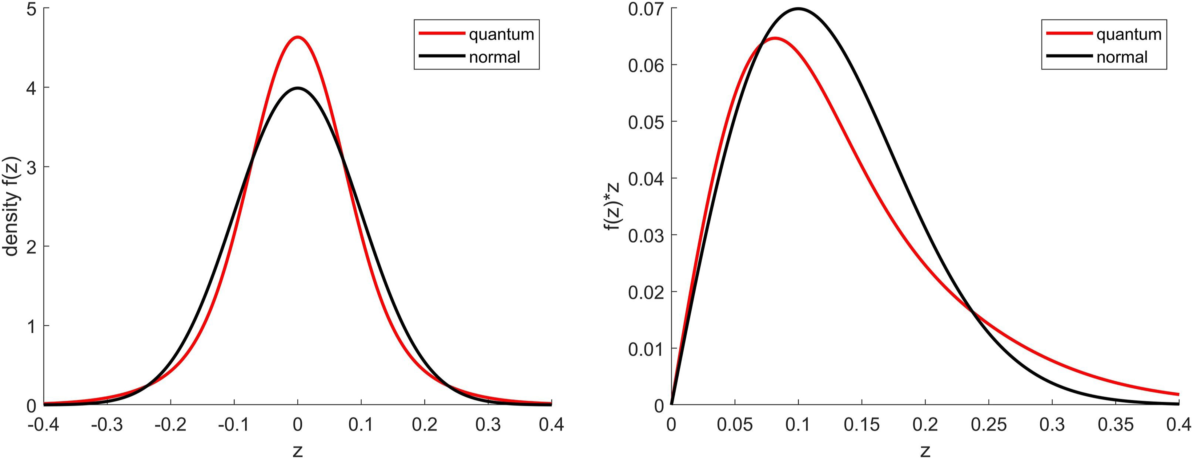 $λ = 0.5$ ) and classical ( $λ = 0$ ) probability distributions. Right panel shows the corresponding probability-weighted payout curves for an ATM call option as a function of relative price change z. The areas under the curves correspond to the expected payouts, which differ by a factor $q (λ)$ .

Another feature of the quantum model, which has been verified experimentally for a range of data sets including historical index data for the S&P 500 and Dow Jones Industrial Average (Orrell, 2024; Orrell & Richards, 2023), is that variance over a period is related to price change over the same period by the simple quadratic equation

σ_{x}^{2} = σ_{0}^{2} + \frac{x^{2}}{2 T} = \frac{σ_{a}^{2}}{2 λ + 1} + \frac{z^{2}}{2}

(2)

where

x

is log price change,

z = x / \sqrt{T}

, and

σ_{0} = σ_{a} / \sqrt{2 λ + 1}

is the minimum volatility. If we define the payout-implied volatility

σ_{p}

to be the volatility in the Black-Scholes model which yields the correct price of a call option for the quantum model, then as discussed in the Appendix, we can write

σ_{p}

in a similar form as

σ_{p}^{2} = q^{2} σ_{a}^{2} + (1 - q^{2}) z^{2}

(3)

where

q = 0.95

and we have assumed for simplicity that the risk-free growth rate and dividend rate are both zero.

Note that the complexity of the derivation in the Appendix comes about because we are trying to use non-normal data to derive the correct volatility to use in an option-pricing model which assumes normality. For the case of an ATM option, as seen in the right panel of Figure 1, the net difference between the classical and quantum models is quite small, and the expected payouts can be made the same by adjusting the standard deviation of the classical curve so that it equals

σ_{b} = q σ_{a} = q σ_{0} \sqrt{2 λ + 1} .

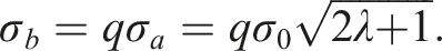
In general, the payout-implied volatility curve is a flattened version of the actual volatility curve that exists in the price data (Figure 2). An example of how the smile curve can be used to fit historic option data is shown in Figure 4 below.

Figure 2.

Blue line shows actual volatility for quantum model with 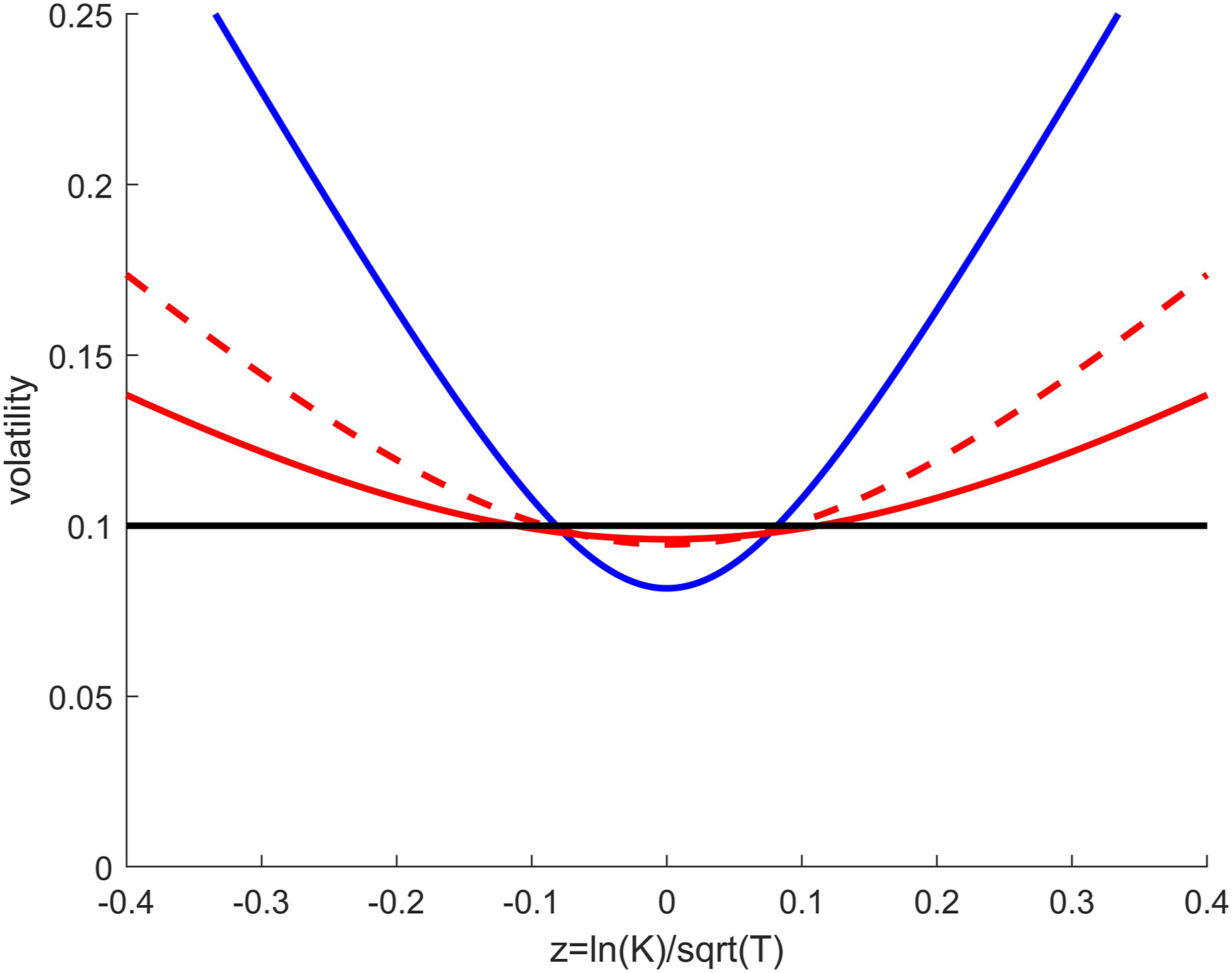$λ = 0.25$ . Red lines show payout-implied volatility for $λ = 0.25$ (solid line) and $λ = 1$ (dashed). Black line shows RMS volatility which is set to $σ_{a} = 0.1$ . The dashed red line (payout-implied for $λ = 1$ ) approximately splits the difference between the blue (actual for $λ = 0.25$ ) and black (constant) lines. As discussed in the Appendix, the curves all intersect near $z = \pm σ_{a} = \pm 0.1$ .

3. What are you Implying?

The discussion so far has focused on two types of volatility: the actual volatility, and the payout-implied volatility, which gives the correct option pricing on average when used as input to the Black-Scholes formula for model price data. If price data is from a lognormal model, then both the actual and the payout-implied volatility are flat. If the data is from the quantum model, or from actual market data, then the actual volatility follows a smile shape, and the payout-implied volatility is a flattened version of the smile. If the risk-free rate used in the Black-Scholes model is lower than the actual growth rate, then this will tend to distort the results.

Note that the payout-implied volatility gives the expected payout for a near-ATM option on the assumption that markets have an average energy level. It therefore accounts for the non-normal distribution of price changes, but not for the distinct relationship between imbalance, price change, and volatility. If we assume instead that the energy level of the market will depart from its average level over the period of interest, then this will affect the expected payout. Beliefs about volatility are therefore conditional on the expected state of market imbalance. This brings us to a third type of volatility, which is the implied volatility that is derived by fitting the Black-Scholes model to the market price that is paid for options. If markets were efficient, as assumed by the Black-Scholes model, one might think that this would equal the payout-implied volatility. The well-known implied volatility smile (Derman & Miller, 2016) can indeed be seen as an attempt to approximate the payout-implied volatility (though this connection is not commonly made), but it is not the same thing and is shaped by a number of factors.

One factor is the actual volatility which applies at the strike price. Because price change and volatility are related through market imbalance, a bet on a particular price change is also a bet on volatility. For example if an investor thinks that markets will be out of balance so volatility will be high and price will increase, then they might decide to purchase a far out-of-the-money option. On the other hand an investor who believes that markets will remain balanced would be more likely to purchase an at-the-money option. Since the price they are willing to pay will depend on their perception of future volatility, the effect will be to lift prices for out-of-the-money options relative to at-the-money options.

The choice of volatility will be modulated also by the particular option strategy; for example an ATM iron butterfly strategy might focus on the actual volatility which applies at the central strike where the payout is concentrated, while a straddle will integrate the payouts on either side. In general, the connection between strike price and market imbalance means that the implied volatility will tend to be more accentuated than the payout-implied volatility, and closer to the actual volatility. The fact that implied volatility is not the same as payout-implied volatility does not necessarily mean that traders are on average mispricing the expected payouts, because again the prices are conditional on imbalance.

While the smile seen with actual volatility finds a clear echo in implied volatility, the latter will also be affected by the presumption of a constant volatility, which – as a core tenet of the dominant pricing model – will tend to limit deviations from a central value. We might therefore expect the the implied volatility to represent a compromise between the actual volatility, and a constant volatility.

Implied volatility will also be shaped by subjective factors such as loss aversion. Indeed, the volatility smile is often assumed to reflect a fear of excess volatility or market crashes; MacKenzie & Millo (2003) for example explain its emergence as a reaction to the 1987 Black Monday crash (another way to look at is that markets woke up to the fact they can be out of balance). Put-call parity should mean that the implied volatilities for put and call options are the same, however puts often have a higher implied volatility than calls, perhaps because they are viewed as insurance against crashes. When the results are merged using a fitting routine, the effect is to produce an apparent skew, so the minimum volatility is displaced to the right. Also, while the approach here assumes that returns are unimodal, investor perceptions of the future may follow a different pattern, and in fact there is evidence that a better model can be obtained using a bimodal quantum walk distribution which affects the shape of the volatility smile and introduces a dependence on expiration date (Orrell, 2021). Another type of distortion is due to the assumption in the Black-Scholes model that the growth rate should be equal to the risk-free rate, which as seen below also tends to shift the volatility smile to the right.

The implied volatility can therefore be viewed as a compromise between these multiple effects. While implied volatility can be modelled in many ways (Derman & Miller, 2016), as seen next a simple approach consistent with the quantum framework is to select an energy level $λ$ and a degree of shift which approximately matches the observed implied volatility curve. A clearer picture will also emerge when we stand back and consider a wide range of strikes and expirations.

4. Measuring Volatility

As seen so far, the quantum model is inconsistent with the Black-Scholes model in a number of respects. The fact, in the quantum model, that payout-implied volatility is strike-dependent violates the assumption in the Black-Scholes model that volatility is constant. While the Black-Scholes model uses a no-arbitrage argument to assert that the risk-free rate should be used in place of a price growth estimate, this proof assumes that the bid/ask spread on transactions is zero. In contrast the quantum model takes the bid/ask spread as a fundamental level of uncertainty which determines much of the behaviour, so assuming it is zero is equivalent to saying that the uncertainty is zero. And while the Black-Scholes model assumes that markets are efficient, the quantum model allows for systematic errors.

Which model is correct can of course only be determined by empirical data. It is easily seen that volatility over a period is related to price change over the same period, as modelled by equation (2). It can also be checked that when it comes to expected payouts, which is what pricing models are supposed to predict, then what counts is not the risk-free rate, but the actual growth rate. For example the reason that SPX call options tend to out-perform put options (Coval & Shumway, 2001) is that call options do well when markets are growing, and the average growth rate (historically about 11%) is much higher than the risk-free rate used in the standard pricing model. And while the Black-Scholes model assumes that markets are efficient, its use actually leads to distortions in market analysis which contribute a form of inefficiency. An example is the methodology used to compute the Cboe VIX volatility index.

The VIX is based on an algorithm which computes a weighted sum of put and call options at different strike prices. It is often said that the VIX is “model-independent” because it only sums the price of options, instead of explicitly attempting to calculate an implied volatility. Carr and Wu (2006) for example write that the VIX index “is constructed from the price of a portfolio of options and represents a model-free approximation of the 30-day return variance swap rate.” However the formula takes it as given that there is such a thing as a single strike-independent volatility in the first place, and that the relevant growth rate to use is the risk-free rate. Since the former was a main assumption of the Black-Scholes model, and the latter its main conclusion, the VIX index can be viewed as a version or logical consequence of the Black-Scholes model.

Figure 3 shows the effect that the Black-Scholes assumptions have on the volatility calculation, using three datasets: lognormal, quantum, and Cboe. The three rows respectively show option prices, implied volatility, and the terms used in the VIX calculation. Starting on the left with the lognormal data, it has a constant volatility of .11 as shown by the flat line in the second row. In the quantum case (second column) the volatility is described by a flattened smile curve, as shown in the second row. The average energy parameter is set to $λ = 1$ , in order to approximately match the Cboe data. Note this energy level also approximately splits the difference between the actual volatility smile and the constant RMS volatility as shown in Figure 2. The RMS volatility is .11, so is the same as for the lognormal data, and the smile is displaced to the right by about 6%, which produces a smaller shift in the option payouts. The third column shows Cboe option price data taken directly from the Cboe VIX white paper (Cboe, 2019). (Two time periods are used in the Cboe calculation, here we show the options with 37 days to expiry).

Figure 3.

Top panels show option price data, including calls, puts, and straddles, for the three data sets. The blue lines show the option prices computed using the Black-Scholes formula with VIX volatility. Middle panels show implied volatilities, along with the result from the VIX calculation (solid line) which is the same for the quantum and Cboe data. The quantum plot also shows the RMS volatility (dashed line) which is the same as the volatility of the lognormal data. In this case the VIX calculation overestimates the RMS volatility by about 25%. The bottom panels show the contributions of option prices to the VIX calculation. The lognormal plot is symmetrical, but the quantum and Cboe cases are skewed and assign higher weights to options with small strikes.

In the top row, the blue lines show the straddle option prices as computed using the Black-Scholes model with VIX volatility. Of course the fit is perfect for the lognormal case, but for the other cases the Black-Scholes prices are higher than the option payouts, which suggests that the Cboe formula is overestimating the applicable volatility.

The reason for this becomes clear in the bottom row of plots, which show the contributions from individual options to the VIX calculation. While the lognormal case is symmetric, the quantum and Cboe cases assign a much higher weight to lower strike prices. This bias is caused by two things: the curvature of the smile, and its displacement to the right. The first is related to the non-constant volatility, while the second occurs in part because option prices are calculated using the risk-free rate instead of the actual growth rate.

The use of constant volatility and the risk-free rate – which are the core of the classical Black-Scholes/VIX approach – therefore jointly affect the volatility estimate, leading it to be too high. For the quantum case, the VIX calculation result (solid line in second row) is about 25% greater than the RMS volatility (dashed line). While we do not know the RMS volatility which applies for the Cboe data, the vertical displacement of the blue lines in the top panels suggests that the VIX volatility is again too high by a similar amount.

It follows that, just by considering the nature of the Cboe VIX formula, one would expect the Black-Scholes/VIX option prices to be higher than the prices paid by traders, because the VIX volatility is too high relative to implied volatility. This leads to a peculiar effect, because if the VIX volatility is higher than the implied volatilities on which it is based, traders might lift their estimates in response, which in turn would increase the VIX, and so on, until the VIX estimate becomes detached from the relevant value. In reality one would expect the implied volatilities to be a compromise between the higher VIX volatility, whose value is consistent with the standard formula, and the lower payout-implied volatility. In fact something like this can be seen in markets, because the implied volatility approximately splits the difference between these two volatilities, with the result that the Black-Scholes/VIX model overestimates the price of ATM SPX straddles by about 40%, while the price paid by traders reduces the error by about half (Orrell & Richards, 2023).

This mispricing is illustrated in Figure 4, which compares option prices against expected payouts for historical data, for the Black-Scholes/VIX model (blue) and the quantum model (red). The quantum model has an average energy of $λ = 0.25$ and is computing using the normalised standard deviation of monthly returns for volatility. If instead the VIX is used for volatility, then from equation (1) we would need to set $λ = 0.5$ in order to capture the difference between RMS volatility (about .15) and the RMS VIX (.21).

Figure 4.

Plot of option prices versus normalised strike price for S&P 500 index data (1992–2022). Blue line shows the Black-Scholes straddle price using the VIX for volatility, red line shows the quantum model with 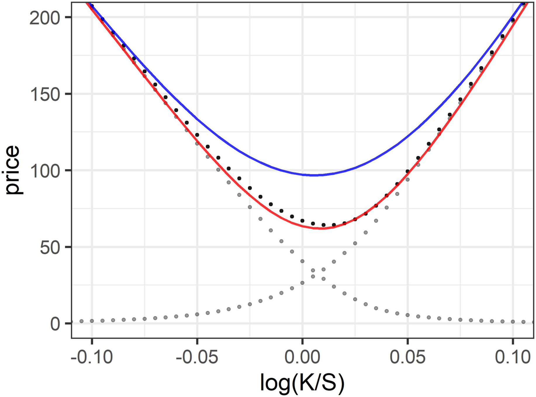$λ = 0.25$ , dots are the average payouts for calls, puts, and straddles.

Indeed, the conclusion that VIX overestimates volatility, and therefore leads to mispricing, can be reached more easily just by noting that what counts when pricing 1-month options is the annualised standard deviation of monthly returns, which is lower than the VIX by about 40% (Ahmad & Wilmott, 2005; Orrell, 2023b). As an example, applying the Black-Scholes formula we find that the approximate value of an at-the-money straddle option for a period of $T$ days and volatility $σ$ is $C ≅ \sqrt{2 T / π} σ$ . However if the VIX is used as an estimate for volatility, then the option price is better approximated by $C ≅ \sqrt{T / π} σ$ .

It might seem unlikely that a widely-used formula which has long been hailed for its empirical accuracy could be out by such a large amount, especially since the quantum payout-implied volatility shows only a moderate degree of strike-dependence. However the VIX index effectively gives a poll of implied volatilities, which as mentioned above can be viewed as bets on market imbalance (or energy level). It therefore makes sense that the 40% error for ATM options is about the same as the spread between the lowest actual volatility and the RMS volatility in the quantum model, since this defines a range of plausible volatility estimates over different strikes and energy levels.

Results can be greatly improved for a range of strikes by assuming in the Black-Scholes model that the risk-free rate equals the average growth rate, and the volatility is about equal to the RMS volatility rather than the VIX; however both these changes involve making uncertain estimates, and neither make sense in the Black-Scholes framework. A first step towards better option pricing therefore is to let go of the classical assumptions and adopt a quantum viewpoint, which takes uncertainty as its starting point.

As a final point, it is interesting to note that the quantum model of volatility in equation (3) is a better match for implied volatility when we take a bird’s eye view over a large range of strikes and expirations. Figure 5 is a heat map of implied volatilty as a function of $x / \sqrt{T}$ for options on the S&P 500 over the period 2004–020. Put options are used for $x < 0$ and calls for $x \geq 0$ . Option prices are averaged over each strike and expiration, and the implied volatility is computed assuming a constant risk-free rate for each year (this has little effect on the results). Expirations $T$ range from 5 days to three years. The quantum model (red line) predicts that implied volatility should asymptote to a line with slope $\sqrt{1 - q^{2}} ≅ 0.3$ , which is in good agreement with the data.

Figure 5.

Heat map of implied volatility as a function of 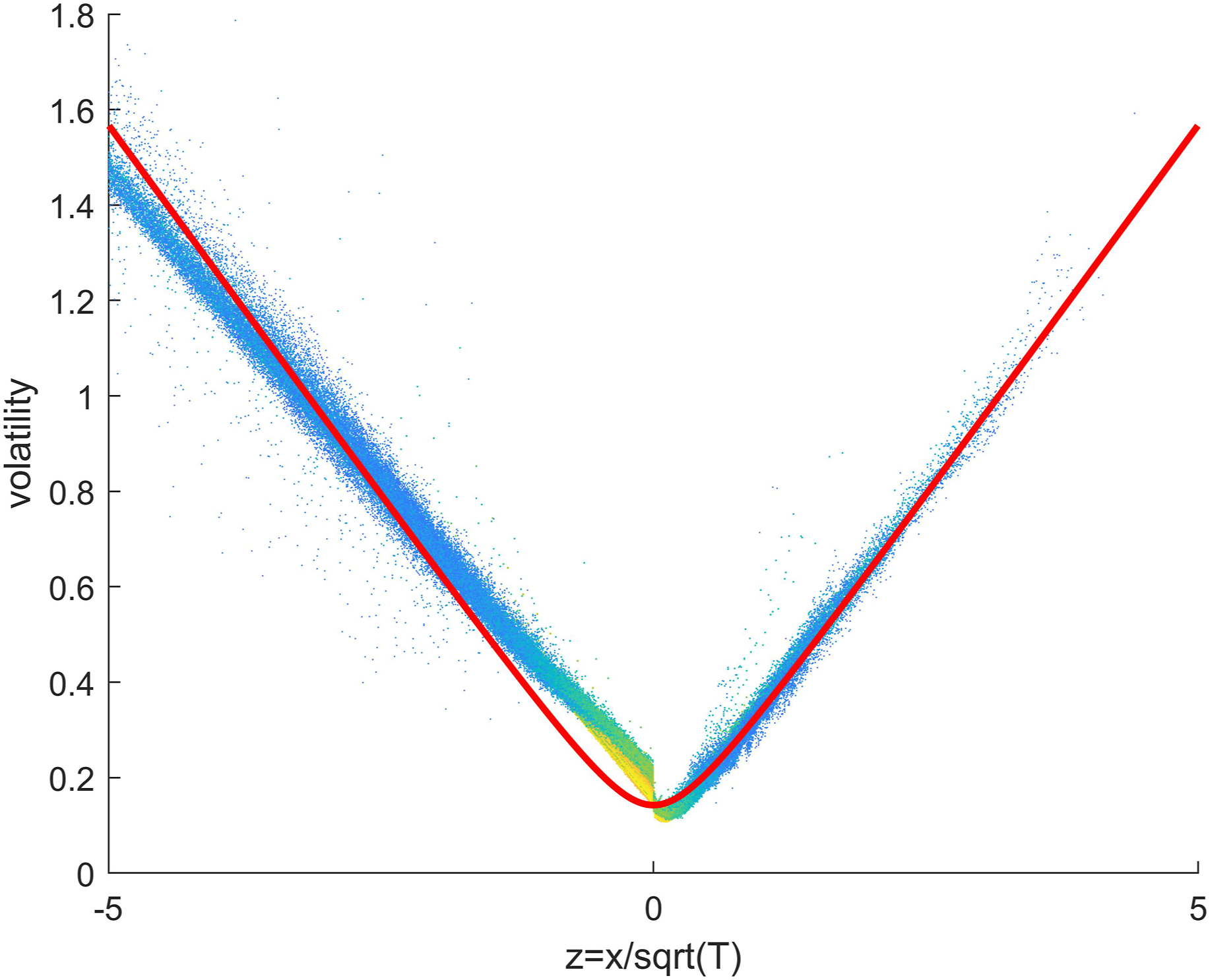$z = x / \sqrt{T}$ for options on the S&P 500 over the period 2004–2020. Put options are used for $x < 0$ and calls for $x \geq 0$ . Option prices are averaged over each strike and expiration, and the implied volatility is computed assuming a constant risk-free rate for each year. Expirations $T$ range from five days to one year. Quantum model with $q = 0.95$ is shown by the red line.

5 . Conclusions

The Black-Scholes model is central to the field of quantitative finance, and has shaped how practitioners and theorists alike price options and think about risk in general; however it is based on a classical random walk model which does not accurately represent the behaviour of markets. The quantum oscillator model replaces the static lognormal price distribution with a dynamic wave function which captures effects such as the relationship between market imbalance, price change, and volatility. Because the quantum model predicts that volatility is strike-dependent, and is driven to a large extent by the bid/ask spread, the theoretical justification of the Black-Scholes formula does not apply.

Perhaps the main advantage of the quantum model is that, by providing an alternative modelling framework, it forces us to question the classical assumptions behind not just the Black-Scholes model, but also related models such as the one used to calculate the VIX volatility index. As we have seen, the Black-Scholes/VIX framework systematically misprices commonly-traded options by around 40%. Since the proof of the Black-Scholes model assumed market efficiency, it is ironic that its use contributed to systematic errors in the pricing of options. It is also puzzling, after half a century, that this mispricing is not common knowledge (see Orrell, 2023a for a discussion). Even when the error is acknowledged, it tends to be ascribed to something other than the model. For example the mispricing of straddle options can be framed as a “volatility risk premium” since straddles protect against volatility (Coval & Shumway, 2001; Goltz & Lai, 2009), but the option-pricing formula is supposed to predict expected payouts, not the subtle emotions of traders.

It is often said that the main appeal of the Black-Scholes model is its simplicity, however the reality is that it was no simpler than the model proposed by Boness a decade earlier; instead its distinguishing feature was its use of the risk-free rate which created a veneer of certainty. By this criterion the quantum model appears to be a step backward, since it replaces the constant volatility with a smile curve, and the risk-free rate with an estimated growth rate. However as already mentioned, much of the apparent complication comes about because non-normal price behaviour is being shoe-horned into a model which assumes normality. In fact the only additional parameter, on which the results are rather weakly dependent, is a measure of average energy.

In terms of structure and complexity, the oscillator is just the quantum version of a spring with a linear restoring force, so can be considered a first-order approximation to a range of processes. Its key properties include a rate of rotation which controls energy; discrete observed energy levels; and a variance which depends on energy level. Displacement increases the average energy, and leads to a Poisson-distributed range of observed energy states. When energy level is identified with the number of representative transactions over a certain period, these properties turn out to be ideal for modelling market behaviour.

The random walk model was invented over a century ago, and reached its peak fifty years ago with the publication of the Black-Scholes model, but has now run (or walked) its course. It is interesting to note that Bachelier’s 1905 thesis coincided with the peak of the quantum revolution in physics. It is long overdue that some of that quantum mathematics, along with its emphasis on uncertainty, found its way into finance.

Footnotes

Acknowledgements

Thanks to Larry Richards for useful discussions and for shared option price data, and to two anonymous reviewers for their helpful comments.

Declaration of Conflicting Interests

The author(s) declared no potential conflicts of interest with respect to the research, authorship, and/or publication of this article.

Funding

The author(s) received no financial support for the research, authorship, and/or publication of this article.

ORCID iD

David Orrell

Appendix

This appendix derives equation (3) for the payout-implied volatility of the quantum model. Suppose that we wish to calculate the payout of an at-the-money (ATM) call option, where we assume for simplicity that the risk-free growth rate and dividend rate are both zero. The payout function is given by the positive part of the final price. Let $x$ be the log price change after a time $T$ and define the normalised price change to be $z = x / \sqrt{T}$ . The expected payout for a lognormally distributed price change with standard deviation $σ$ is then

C_{c} = \int_{0}^{\infty} z f (z) d z = \frac{σ}{\sqrt{2 π}}

where

f (z)

is the normal distribution with standard deviation

σ

. (More correctly, we should express the payout in terms of the normalised strike price

K = e^{x}

but the answers are nearly identical.) This integral is the area under the curve shown in the right panel of Figure 1 in the main text.

The quantum price change distribution, in contrast, can be viewed as a Poisson-weighted composite of normal curves, whose variances $σ_{n}$ correspond to energy levels $n$ . The motivation for this model is that price is perturbed randomly as in the classical model, but the volatility at each step depends on the energy level. The expected payout is therefore

C_{q} = \sum_{n} w_{n} \frac{σ_{n}}{\sqrt{2 π}}

where

σ_{n}

is the volatility of the state with energy number

n

, and

w_{n} = \frac{λ^{n}}{n!} e^{- λ}

is the corresponding Poisson weighting. From equation (1), the standard deviation of the quantum curve satisfies

σ_{a}^{2} = (2 λ + 1) σ_{0}^{2}

, and the ratio of quantum to classical payout is

q = \frac{C_{q}}{C_{c}} = \sum_{n} w_{n} \frac{σ_{n}}{σ_{a}} = \sum_{n} w_{n} \frac{\sqrt{2 n + 1}}{\sqrt{2 λ + 1}}

As seen in the right panel of Figure 1, the expected payout from the quantum model is lower for small strikes but higher for larger strikes, so the net difference between the classical and quantum formulae is quite small. The payouts (which again are for ATM options) can be made the same by adjusting the standard deviation so that it equals

σ_{b} = q σ_{a} = q σ_{0} \sqrt{2 λ + 1}

If we now assume that the payout-implied volatility follows a similar form as the actual volatility (equation (2)), we can write

σ_{p}^{2} = σ_{b}^{2} + \frac{s^{2} z^{2}}{2}

where we assume for now that the curve is symmetric so the linear term is zero (alternatively this can be viewed as a second-order Taylor expansion for variance). Let

C (K)

be the cost of a call option at strike

K

, and

P_{b} = \frac{1}{σ_{b} \sqrt{2 π}} = \frac{1}{q σ_{0} \sqrt{2 π (2 λ + 1)}}

be the peak of a normal curve with standard deviation

σ_{b}

. Then it can be shown that the curvature of the cost function is

\frac{d^{2} C}{d^{2} K} = f (K, T) = P_{b} (1 + \frac{s^{2}}{2})

where

f (K, T)

is the log price probability density and again we assume the risk-free and dividend rates are zero. The peak of the quantum distribution is given by

P_{q} = \sum_{n} w_{n} \frac{1}{σ_{n} \sqrt{2 π}} = \sum_{n} w_{n} \frac{1}{σ_{0} \sqrt{2 π (2 n + 1)}}

so the ratio is

\frac{P_{q}}{P_{b}} = q p

where

p = \sum_{n} w_{n} \frac{\sqrt{2 λ + 1}}{\sqrt{2 n + 1}}

If the curvatures of the cost functions for the quantum and normal cases are to be the same, it follows that the smile coefficient $s$ should satisfy

1 + \frac{s^{2}}{2} = \frac{P_{q}}{P_{b}} = q p

s = \sqrt{2 q p - 2}

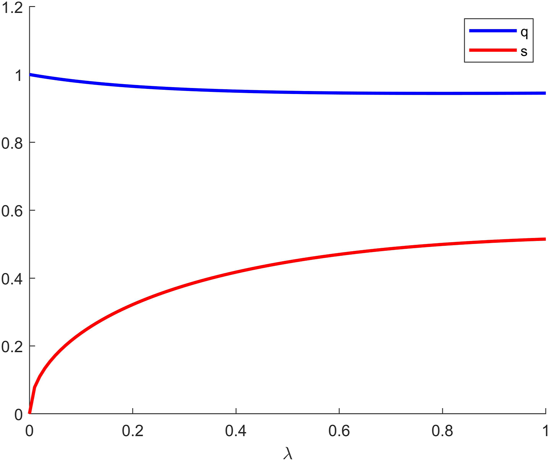
. The equation for the payout-implied volatility as a function of

z

is therefore (A1)

σ_{p}^{2} = σ_{b}^{2} + \frac{s^{2} z^{2}}{2} = q^{2} σ_{a}^{2} + (q p - 1) z^{2}

For $λ$ in the range of 0–1, $q$ is in a range of 1 to about .94. Setting $λ = 0.25$ gives $q = 0.96$ and $s = 0.35$ , while $λ = 0.5$ gives $q = 0.95$ and $s = 0.45$ (see Figure A1).

It can be shown numerically that for $λ$ in the range 0–1, we have

\sqrt{q^{2} + \frac{s^{2}}{2}} ≅ 1

so equation (A1) can be simplified to

σ_{p}^{2} = q^{2} σ_{a}^{2} + \frac{s^{2} z^{2}}{2} ≅ q^{2} σ_{a}^{2} + (1 - q^{2}) z^{2}

which is equation (3) in the main text.

Setting $z = σ_{a}$ in this equation gives $σ_{p} ≅ σ_{a}$ . Similarly, the actual volatility at this point from equation (2) is

σ_{x}^{2} = σ_{0}^{2} + \frac{z^{2}}{2} = \frac{σ_{a}^{2}}{2 λ + 1} + \frac{σ_{a}^{2}}{2} = σ_{a}^{2} (\frac{2 λ + 3}{4 λ + 2})

σ_{x} ≅ σ_{a}

for

λ

in the range of .25–.5. In other words, at a normalised displacement

z = σ_{a}

, both the payout-implied volatility and the actual volatility are about equal to the RMS volatility.

Figure A1.

Plot showing the parameters $q$ and $s$ from equation (A1) as a function of $λ$ .

References

Ahmad

Wilmott

(2005). Which free lunch would you like today, sir? Delta hedging, volatility arbitrage and optimal portfolios. Wilmott, 2005(November), 64–79.

Ahn

Choi

M. Y.

Dai

Sohn

Yang

(2017). Modeling stock return distributions with a quantum harmonic oscillator. EPL, 120(3), 38003. https://doi.org/10.1209/0295-5075/120/38003

Bagarello

(2006). An operatorial approach to stock markets. Journal of Physics A, 39(22), 6823–6840. https://doi.org/10.1088/0305-4470/39/22/001

Black

Scholes

(1973). The pricing of options and corporate liabilities. Journal of Political Economy, 81(3), 637–654.

Boness

A. J.

(1964). Elements of a theory of stock-option value. Journal of Political Economy, 72(2), 163–175.

Carr

(2006). A tale of two indices. Journal of Derivatives, 13(3), 13–29. https://doi.org/10.2139/ssrn.871729

Cboe . (2019). Cboe volatility index.

Clark

(director) (1999) The midas formula (motion picture).

Coval

J. D.

Shumway

(2001). Expected option returns. The Journal of Finance, 56(3), 983–1009. https://doi.org/10.1111/0022-1082.00352

10.

Derman

Miller

M. B.

(2016). The volatility smile. John Wiley & Sons.

11.

Fama

E. F.

(1965). Random walks in stock-market prices. Graduate School of Business, University of Chicago.

12.

Gao

Chen

(2017). A quantum anharmonic oscillator model for the stock market. Physica A: Statistical Mechanics and its Applications, 468(C), 307–314. https://doi.org/10.1016/j.physa.2016.10.094

13.

Gatarek

(2023). The principle of two models: The cases of Black-Scholes formula for interest rates and of Gaussian copula for credit. Wilmott, 2023(125), 125. https://doi.org/10.54946/wilm.11131.

14.

Goltz

Lai

W. N.

(2009). Empirical properties of straddle returns. The Journal of Derivatives, 17(1), 38–48.

15.

Gonçalves

C. P.

Gonçalves

(2008). An evolutionary quantum game model of financial market dynamics – Theory and evidence. Available at: https://ssrn.com/abstract=982086

16.

Haven

Khrennikov

Robinson

(2017). Quantum methods for social science: A first course. World Scientific.

17.

Khrennikova

Patra

(2019). Asset trading under non-classical ambiguity and heterogeneous beliefs. Physica A, 521(C), 562–577. https://doi.org/10.1016/j.physa.2019.01.067

18.

Lee

R. S. T.

(2021). Quantum finance forecast system with quantum anharmonic oscillator model for quantum price level modeling. International Advance Journal of Engineering Research, 4(02), 01–21. https://doi.org/10.1007/978-981-32-9796-8

19.

MacKenzie

Millo

(2003). Constructing a market, performing theory: The historical sociology of a financial derivatives exchange. American Journal of Sociology, 109(1), 107–145. https://doi.org/10.1086/374404

20.

Meng

Zhang

J.-W.

Guo

(2016). Quantum brownian motion model for the stock market. Physica A: Statistical Mechanics and its Applications, 452(2016), 281–288. https://doi.org/10.1016/j.physa.2016.02.026.

21.

Meng

Zhang

J.-W.

Guo

(2015). Quantum spatial-periodic harmonic model for daily price-limited stock markets. Physica A: Statistical Mechanics and its Applications, 438(2015), 154–160. https://doi.org/10.1016/j.physa.2015.06.041.

22.

Merton

R. C.

(1990). Continuous-Time Finance. Cambridge, MA: Basil Blackwell.

23.

Orrell

(2021). A quantum walk model of financial options. Wilmott, 2021(112), 62–69. https://doi.org/10.1002/wilm.10918

24.

Orrell

(2022). Quantum economics and finance: An applied mathematics introduction (3rd ed.). Panda Ohana.

25.

Orrell

(2022a). Market impact through a quantum lens. Wilmott, 2022(122), 50–52. https://doi.org/10.54946/wilm.11072

26.

Orrell

(2023a). The Black-Scholes magic trick, explained. Wilmott, 2023(126), 90–93. https://doi.org/10.54946/wilm.11153.

27.

Orrell

(2023b). Fix the VIX: A quantum perspective on the fear index. Wilmott, 2023(127), 48–50. https://doi.org/10.54946/wilm.11168.

28.

Orrell

(2024) A quantum oscillator model of stock markets. Quantum Economics and Finance 1 (in press).

29.

Orrell

Richards

(2023). Keep on smiling: Market imbalance, option pricing, and the volatility smile. Wilmott, 2023(124), 58–64. https://doi.org/10.2139/ssrn.4205729

30.

Ross

S. A.

(1987). Finance. In Eatwell

Milgate

Newman

(Eds.), The new palgrave: A dictionary of economics (Vol. 2). Macmillan.

31.

Rubinstein

(1994). Implied binomial trees. Journal of Finance, 49(3), 771–818.

32.

Schaden

(2002). Quantum finance. Physica A, 316(1), 511–538. https://doi.org/10.1016/S0378-4371(02)01200-1

33.

Simons

(1997). Model error. New England Economic Review, 1(Nov), 17–28.

34.

Wilmott

(2010). Frequently asked questions in quantitative finance. Wiley.

35.

Huang

(2008). Non-classical oscillator model for persistent fluctuations in stock markets. Physica A: Statistical Mechanics and its Applications, 387(5–6), 1255–1263. https://doi.org/10.1016/j.physa.2007.10.050

Quantum Uncertainty and the Black-Scholes Formula

Abstract

Keywords

1. Introduction

2. The Quantum Smile

3. What are you Implying?

4. Measuring Volatility

5 . Conclusions

Footnotes

Acknowledgements

Declaration of Conflicting Interests

Funding

ORCID iD

Appendix

References