Sage Journals: Discover world-class research

Abstract

Court congestion is among society’s oldest legal problems; protections from it are enshrined in constitutions around the world. This paper uses publicly available data on the duration of millions of criminal court cases over the course of two decades across Canadian provinces to analyze the performance of the criminal justice system using queueing theory. Our new approach to estimating the delay of criminal trials appropriately includes the time from the point the charges are laid to first appearance, which is not available in raw data. We find that the queue sizes and wait times are growing in many provinces, suggesting that the criminal justice system is approaching, or perhaps beyond, capacity. Using several different time series specifications, we find that the utilization rate and model-implied queue size co-move positively with the population in pretrial custody. The results suggest that court congestion, as measured by statistics from queueing theory, has explanatory power for the rising population in pretrial custody.

Keywords

criminal law criminal procedure constitutional law queueing theory time series

And cases like this can last a long time, especially the ones that have been coming up lately.

—Franz Kafka, The Trial

1. Introduction

Court congestion is among society’s oldest legal problems. We are told that in 42 A.D. the Emperor Claudius exhorted the Roman Senate to pass a law introducing a summer session into the congested Roman courts;¹ in 1215, King John promised in the famous and enduring clause 40 of the Magna Carta “[t]o no one will we sell, to no one deny or delay, right or justice” [emphasis added];² Shakespeare’s Hamlet lists ‘law’s delay’ (3.1.82) fifth in his seven burdens of man;³ Kafka’s early 20th century critique of Austro-Hungarian criminal procedure makes immediate mention of the phenomenon. The list goes on.

While the problem is an old one, it remains among the most the important legal problems today, proving its stubbornness. As of late, court delay has given rise to constitutional concerns in Canada, notably in R v. Jordan,⁴ making the subject particularly relevant to the present moment. The framework in Jordan attempts to address what the Supreme Court of Canada called a “culture of complacency within the system towards delay” (at para. 4) by clearly defining the total duration of a case and how to calculate delay and then establishing presumptive ceilings on the duration of trials. Our theoretical approach allows us to infer the time from the point charges are laid to first appearance to fully account for what has become known as the “Jordan clock,” improving on existing measurements using raw data.⁵ Moreover, central measures from queueing theory, such as the server-level utilization rate, queue size, and wait time co-move positively with the population in pretrial custody.⁶ This suggests that court congestion, as measured by statistics from queueing theory, has predictive power for the secular rise in the population in pretrial custody across Canadian provinces.

Indeed, the right to trial within reasonable time is enshrined in the Sixth Amendment of the United States Constitution under the Speedy Trial Clause and in Section 11(b) of the Canadian Charter of Rights and Freedoms.⁷ Constitutional protections from unreasonable delay are well-founded. Canada’s Charter protects the accused’s security, liberty, and fair trial interests, which keeps the accused from a trial or bail being held over their head for unreasonable lengths and ensures a trial in which witnesses and evidence are available. These guarantees mitigate the undue costs of prolonged detention in pretrial custody, such as failure to meet employment and housing obligations, deterioration of personal relationships, as well as the ability to prepare a defence. Prolonged delay may also be the product of inadequate administrative resources provided by the State, making constitutional protections necessary to ensure swift justice.

This paper uses publicly available data on millions of criminal court cases over the last two and a half decades in Canada to study the criminal justice system through the lens of a branch of mathematics known as queueing theory, the study of waiting times. We use data on the time lapse of criminal trials from first appearance to final disposition to estimate the service time distribution in days and the total number of charges laid in a given year compute the system’s arrival rate.⁸ The service time distribution fits the exponential distribution well, suggesting that a standard memoryless queueing model could be appropriate.⁹ Using our measure of the average number of cases that arrive per day, the total number of charges laid, and the rate of the service time distribution, we are able to compute the utilization rate, a key performance metric in queueing theory, of each provincial court system. With these estimates and data on the court’s open caseload, we are able to compute measures of the provincial criminal court system’s performance, such as queue size and wait time, using the multiple server queueing model with minimal assumptions. Data on measures such as the time from arrest to first appearance are currently unavailable in existing raw data, making our paper the first to properly estimate the full duration of a criminal proceeding according to the “Jordan clock” established by the Supreme Court of Canada in 2016. We find that the implied measures of queue size and wait time are non-stationary and increasing over our series, suggesting that the court’s backlog is growing and that the criminal justice system may not be able to handle all of the cases before it without substantial delay.

We then use our results from the queueing analysis to examine the extent to which queueing theory’s measures of court congestion can explain the rise of the population in pretrial custody. Several time series regressions detect positive co-movement between queueing theory’s measure of the total number being served, the server-level utilization rate λ_t/μ_t, and the average count of the population in pretrial custody. The model’s measure of queue size L_q is also predictive of the population in pretrial custody, suggesting that our model’s measures perform better than raw data on open caseload. The results indicate that the statistics suggested by queueing theory have predictive content and that court congestion has explanatory power for the rising population in pretrial custody. Indeed, court congestion can help explain the paradox of falling crime with an ascending population in pretrial custody.

1.1. Queueing Theory

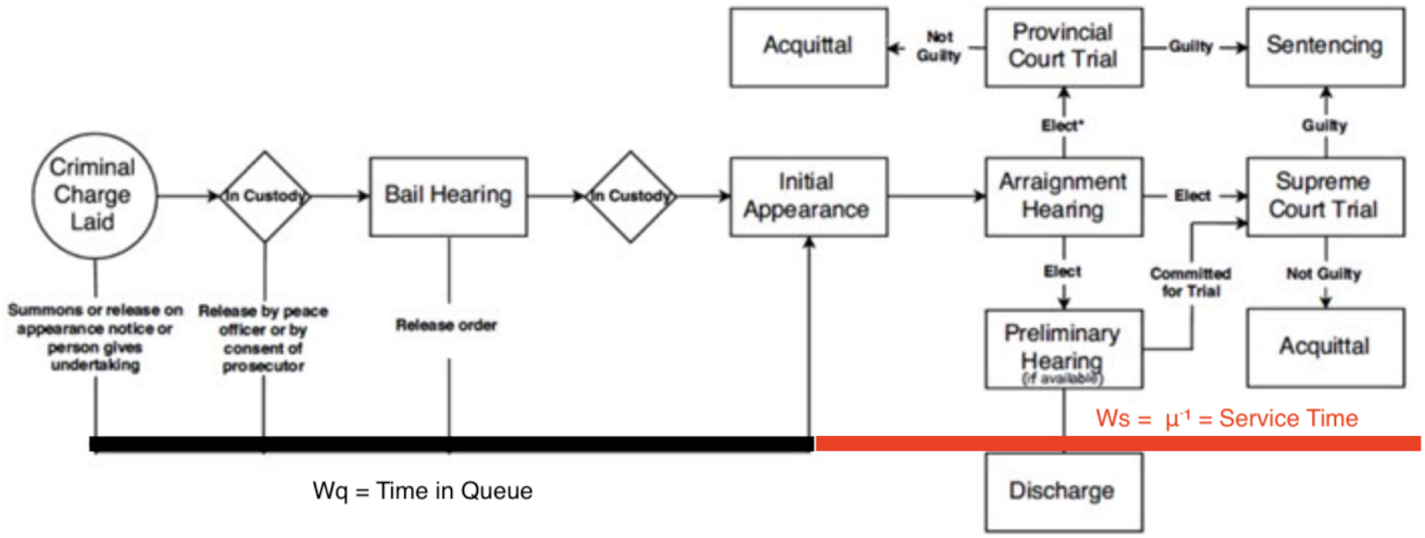
Originally developed to study telephone networks by A.K. Erlang, a Danish engineer who worked for the Copenhagen Telephone Exchange, queueing theory models the arrival and service of customers to provide a mathematical model through which to analyze the performance and equilibrium of a service system, like courts, such as the length of a waiting line, or queue, and average waiting times (Hlynka, 2017). Loosely speaking, queueing theory is the mathematical theory of lineups. Ross (2010) describes a queueing model as a model “in which customers arrive in some random manner at a service facility. Upon arrival they are made to wait in queue until it is their turn to be served. Once served they are generally assumed to leave the system.” Queueing theory has been widely successful at modeling congestion in a number of areas. Green (2006) writes that “[m]any organizations, including banks, airlines, telecommunications companies, and police departments, routinely use queueing models to help determine capacity levels needed to respond to experienced demands in a timely fashion.” In the most basic framework,“customers” arrive to a service center according to a homogeneous Poisson process with rate λ and are served first-come first-serve (FCFS) at a time distributed according to the exponential with rate μ. To immediately connect the theory with law and our data, the reader should think of charges being laid as an arrival of a case to the court system, any time leading up to the first appearance as the waiting time, and the service time as the duration of the trial from first appearance to final disposition, where service is the issue of a judgment by the court. A diagram of a multiple-server queuing system with two servers (c = 2) is below in Figure 1. The full criminal trial procedure in Canada can be seen below in Figure 2.

Figure 1.

Multiple-server queuing system with two servers (c = 2).

Figure 2.

Stages in a criminal case. Note. Figure displays criminal trial procedure in Canada. Source: https://www.court.nl.ca/supreme/rules-practice-notes-and-forms/criminal-proceedings/general/.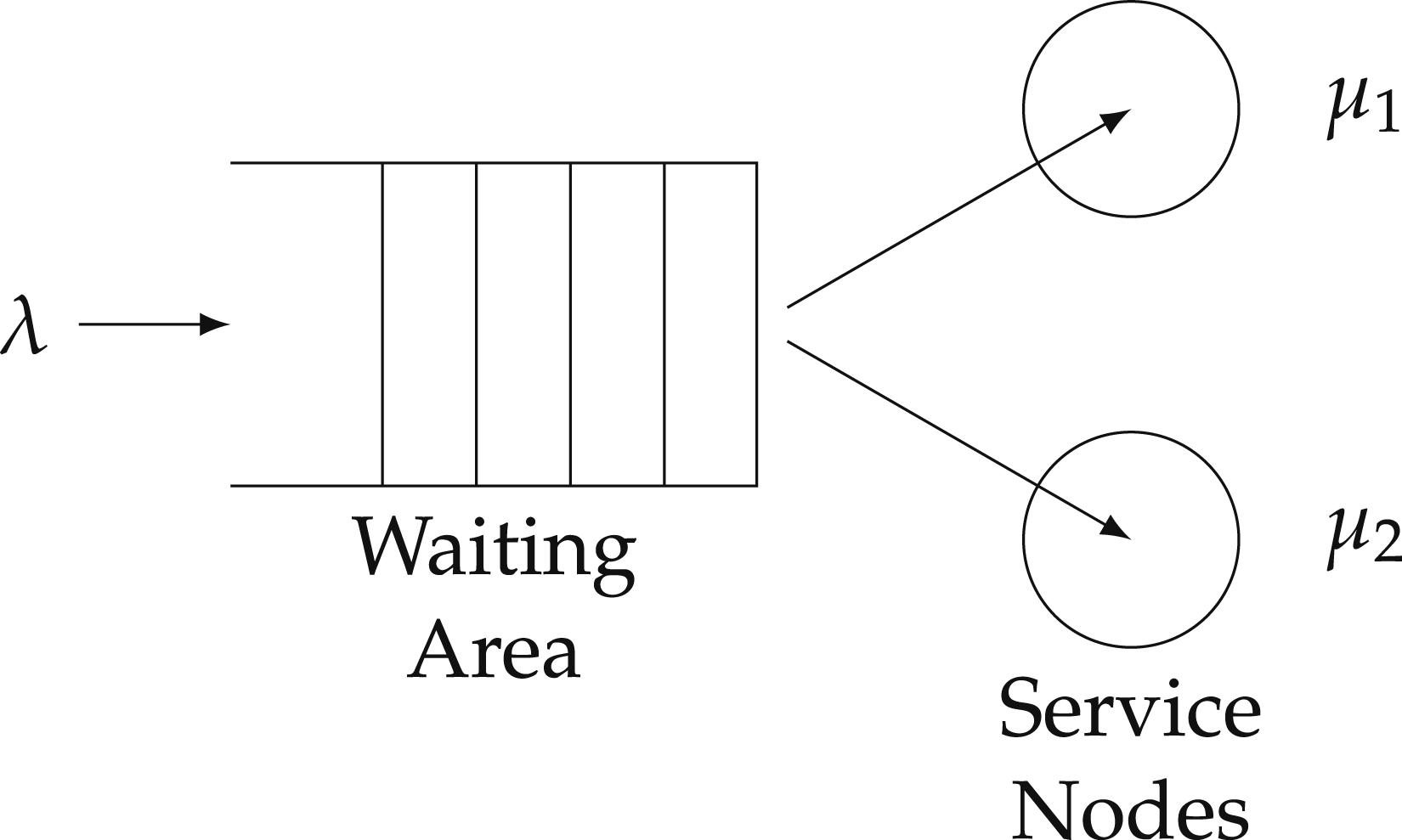

The important inputs to specifying a queueing model are as follows.

(1) The arrival process. The arrival process is a measure of how arrivals occur through time. The most common approach, for its tractability, is to assume that arrivals follow a homogeneous Poisson process, in which customers arrive uniformly through time at the rate of λ arrivals per unit time. However, it can be generalized to other arrival processes. Regardless of how the arrival process is specified, the parameter λ, referred to as the arrival rate, is the average number of arrivals per unit time over the long-run.

(2) The probability distribution of service times. The standard memoryless queueing framework models service times as exponentially distributed in order to exploit memorylessness to generate a Markovian process. However, extensions can accommodate general service time distributions, such as the log normal distribution. In what follows we let the average service time be 1/μ where μ can be interpreted as the number of customers that a single server is capable of serving in one unit of time (assuming the next service begins immediately after the current service is completed).

(3) The number of available servers. In order to determine the number of servers available in a particular legal jurisdiction, one must first have a clear notion of what a server is. In the legal system, a server could be a courthouse, a judge, or a fraction of a judge. We are able to circumvent estimating the number of servers by combining multiple data sources on the system’s performance – arrivals, service time, and the total number in the system – to back out the system’s implied queue size and wait time, allowing us to remain agnostic about the exact number of servers in the system.

(4) The service discipline. Conventional queueing theory models the service discipline as first-come first-serve (FCFS), however extensions of the basic model use priority queueing and processor sharing, just to name a couple. Our paper remains agnostic as to the service discipline. We are able to use identities from queueing theory that do not depend on the service discipline to compute implied measures of system performance given the data we have on the criminal justice system.

The important outputs of the queueing model are the utilization rate, total time in the system, average wait time, and queue size, which are currently not available in conventional data sources, such as the Canadian data that we use. We use queueing theory, in particular, Little’s Law, which holds under extremely general assumptions on the arrival process, the service discipline, and the number of servers, to back out measures of congestion using queueing theory. Little’s Law states that the total number in the system L is equal to the product of the arrival rate λ and the total time in the system W in expectation

L = λ W .

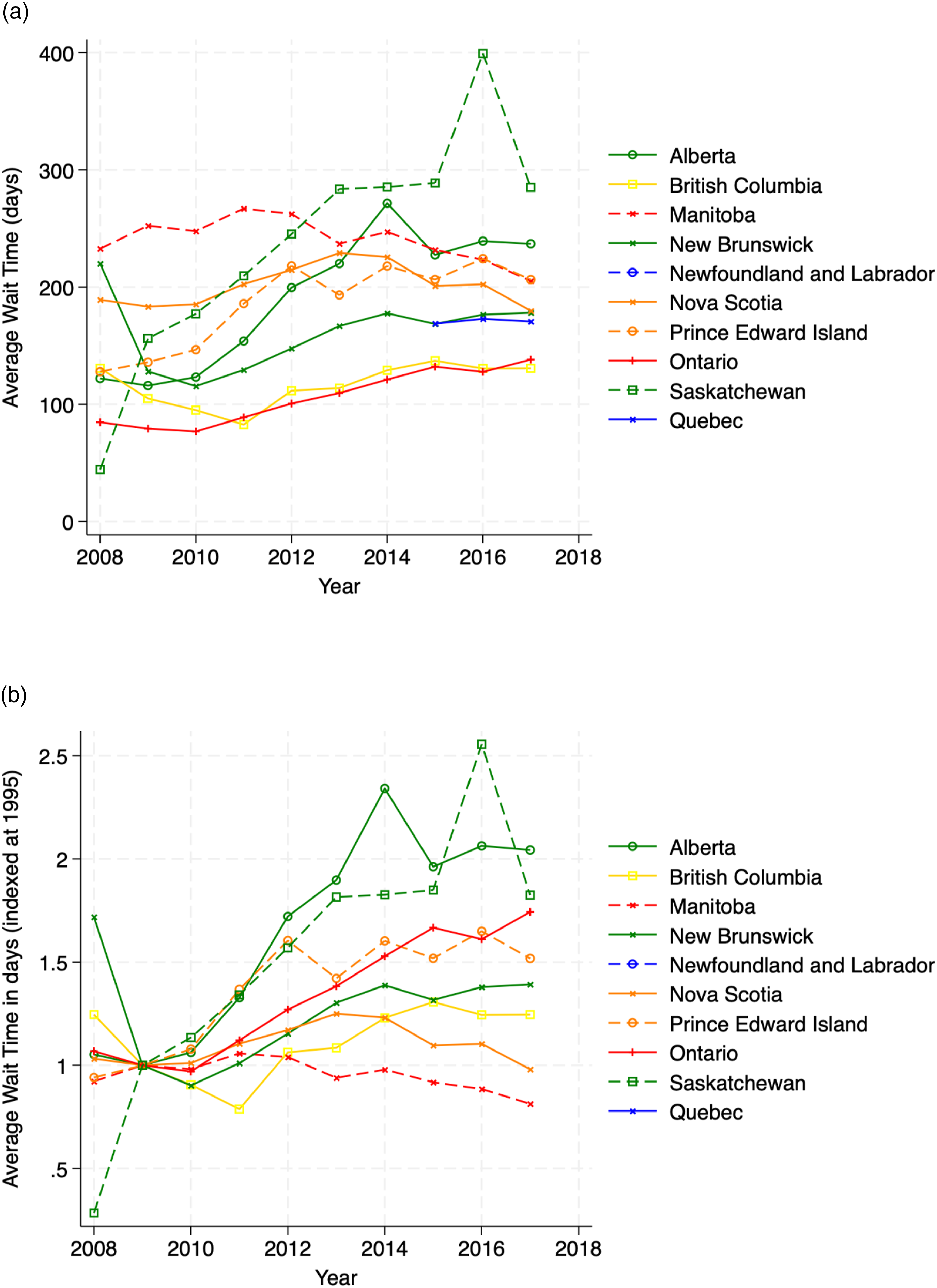
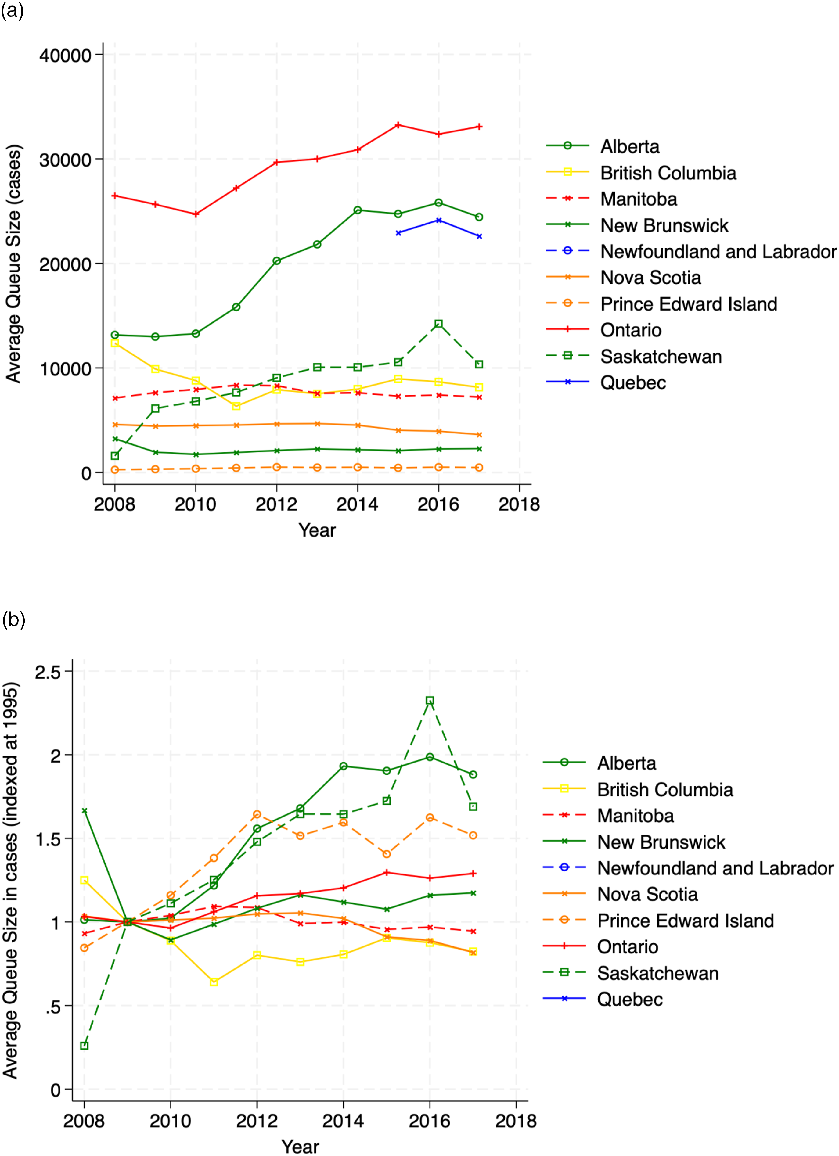
We use data on the open caseload to measure the total number in the system L and the arrival rate λ to back out total time in the system W. To compute the expected or implied wait time we can subtract mean service time μ⁻¹ from total time in the system W. We find that measures of congestion from queueing theory, such as wait time and queue size, are, in many provinces, non-stationary and increasing.

A key performance measure in any queueing model is the utilization rate ρ = λ/μ, which is the arrival rate times the mean service time.¹⁰ Using time series analysis on de-trended and differenced processes, we find strong co-movement between the utilization rate, queueing theory’s measure of traffic, and the population in pretrial custody (remand). The outputs from our model, such as server-level utilization and queue size, outperform conventional measures in the data, such as open caseload, in predicting the rising population in pretrial custody. This suggests that queueing theory has some predictive content for explaining the paradox of a falling crime rate, that is, the arrival rate, and rising population in pretrial custody.

1.2. Related Literature

Relative to other applications of queueing theory, such as healthcare and telephone networks, there has been little academic work using formal queueing theory to study the legal system, even despite the relatively obvious connection between court delays and queueing theory and the deep reliance in constitutional law, at least in Canada, on estimating the time from arrest to first appearance. We combine our estimates of the service time distribution with data on the court’s open caseload to compute conventional measures of performance from queueing theory, such as queue size and time in the queue. We are the first, to our knowledge, to then relate these measures back to the population in pretrial custody. Across several time series specifications, we find that the system’s server-level utilization rate is robustly related to the average count of individuals in pretrial custody, suggesting that court congestion can explain the recent rise in the population in pretrial custody across Canadian provinces. Indeed, the model’s measures of congestion outperform those measures readily available in the data, such as open caseload.

McAllister et al. (1991) first used queueing theory to simulate a five-stage model of the pretrial case processing system from arraignment to trial assignment. Their multi-stage queueing approach is particularly appropriate given the realities of court procedures, but is greedy in terms of the granularity of the data required to perform their exercise. Our approach relies on widely published, aggregate metrics and one basic theorem in queueing theory, that is, Little’s Law (Little, 1961), which does not depend on the arrival process, the number of servers, or the service discipline (Jewell, 1967; Eilon, 1969), to provide a diagnostic of the overall court system in long-run equilibrium by producing measures of performance that are predictive in terms of the population in pretrial custody. Examining behaviour of the queue and the model-implied time to first appearance, we find that wait time and queue size are increasing and non-stationary across provinces.

For the country we analyze, Canada, there has been a troubling rise of the population in pretrial custody, displayed in Figure 3, that one must reconcile with falling crime rates. A novel contribution of our approach is that we find that the measures it produces co-move with the rising population in pretrial custody, resolving this paradox. Thus, our approach has important ties to the focal concerns literature in criminology, and social science more broadly, studying the deleterious effects of court delay for those in pretrial custody, such as faster time to guilty pleas (Petersen, 2020).

Figure 3.

Average population in pretrial custody and mean daily arrivals. Note. Figure plots average annual population in pretrial custody (Source: Canadian Centre for Justice and Safety (CCJS) Correction Key Indicator Report (CKIR)) and mean number of charges per day in a given year (excluding administration of justice offences) (Source: Integrated Criminal Court Survey (ICCS)).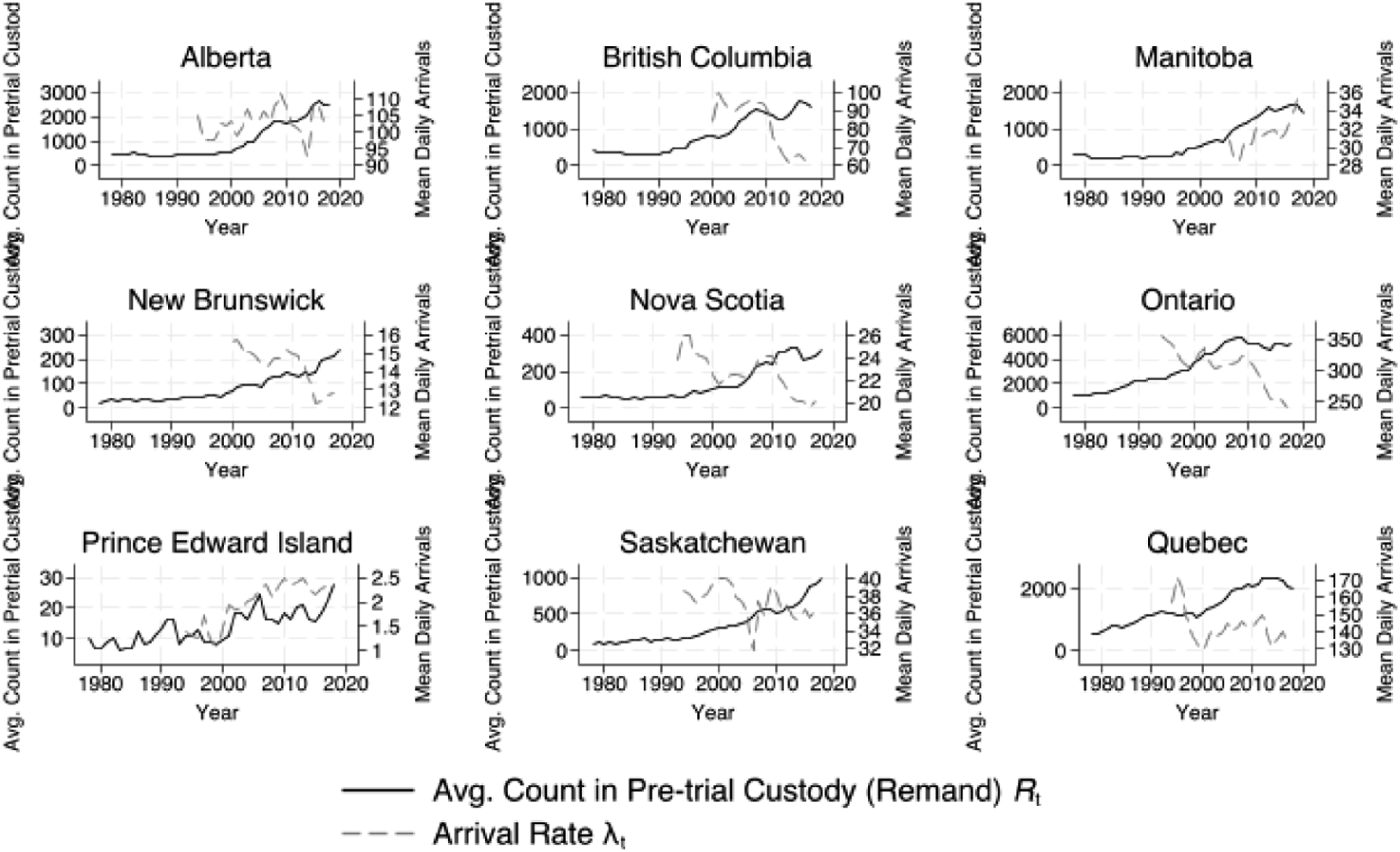

The literature on the link between sentencing, such as guilty pleas, and caseload has found little success. For instance, Yang (2016) finds no relationship between judicial vacancies and delay in the US, but a causal impact of vacancies on guilty pleas. Our approach can help create new measures that outperform measures currently available to researchers, such as open caseload and the arrival rate, in predicting the population in pretrial custody. This contributes to a larger literature on the causes and consequences of pretrial custody. For example, Dobbie et al. (2018), find that pretrial detention significantly increases the probability of conviction, primarily through an increase in guilty pleas, has no net effect on future crime, but decreases formal sector employment and the receipt of employment- and tax-related government benefits. Court congestion can resolve the paradox between rising pretrial populations and falling crime rates.

Mukherjee and Whalen (2018) examine the time lapse between when a case enters a court’s docket and when it is ultimately disposed of using data from the Supreme courts of the United States, Massachusetts, and Canada. The authors find that the underlying distribution of case resolution timing features a slow decay with a decreasing tail, demonstrating that, in each of the courts examined, the vast majority of cases are resolved relatively quickly, while there remains a small number of outlier cases that take an extremely long time to resolve. This paper uses queueing theory to compute statistics on the criminal justice system for nine Canadian provinces (excluding Newfoundland and Labrador). We use the estimate of the service time distribution using the time lapse from first appearance to final disposition with a maximum likelihood procedure. While this approach is consistent with Mukherjee and Whalen (2018), we explicitly interpret this quantity as the distribution of service time.

We find that the distribution of the duration criminal trials is well-fit by the exponential distribution, perhaps lending itself to a workhorse memoryless queueing model. We then use queueing theory to then back out the time from arrest to first appearance, which is of interest to the constitutional framework set out in Jordan. We find that both model-implied queues and wait times are increasing and non-stationary in many provinces. In pooled time series analysis, we find that these quantities of interest are related to the rising population in pre-trial custody.

Our novel approach to estimating the total time for trial comports with the framework as laid out in Jordan. For instance, a study by Karam et al. (2020) attempts to examine prima facie section 11(b) violations under the framework set out in Jordan using the same data publicly available data we use on the time lapse from first appearance to final disposition. However, this ignores the very clear fact set out in the framework established under Jordan that the time under consideration for s. 11(b) violations begins at the time the charges are laid, not the first appearance. Thus, the time from the point charges are laid to first appearance is a quantity of substantial interest, but is only available using data sources that are unavailable to researchers. We use queueing theory to estimate the time from the point the charges are laid to the first appearance. Thus, our new approach to estimating the delay of criminal trials should be incorporated into calculations of the share of cases at risk of violating s. 11(b) per the framework in Jordan.

The paper proceeds in five sections. Section 2 describes the data. Section 3 describes the estimation of the service rate. Section 4 computes the main measures of system performance from the multiple server queueing model. Section 5 uses time series analysis to examine the relationship between the queueing model outputs and the population in pretrial custody (remand). Section 6 concludes.

2. Data

The data used to construct estimates of service time and arrival rates are from Statistics Canada’s Integrated Criminal Court Survey (ICCS). The survey provides data from a dozen administrative databases across Canada from provinces from 1994 to 2019 for most provinces. The data draws on administrative records from provincial-territorial and superior courts in Canada. We focus our analysis the provinces in Canada: Alberta, British Columbia, Manitoba, Nova Scotia, New Brunswick, Ontario, Prince Edward Island, Quebec, and Saskatchewan. In particular, the ICCS case counts are broken down by geography, year, single or multiple charge(s), defendant age group (18+) and sex, and 23 offences, as well as by time lapse from first appearance to final disposition.¹¹ A case that has more than one charge is represented by the charge with the “most serious offence” (MSO).¹²

2.1. Remand

The data on the population in pretrial custody come from the Canadian Centre for Justice and Safety (CCJS) Correction Key Indicator Report (CKIR). The CKIR is an annual administrative data survey. It collects aggregate data on average daily custody counts and month-end supervised community corrections counts in the youth and adult correctional systems. The information provides an overview of adult and youth corrections populations and serves as a basis for calculating incarceration rates. We use the average annual count in pretrial custody (on remand) from 1978 to 2019.

2.2. Caseload

The data on open caseload come from Statistics Canada’s Court Workload Indicators (CWI) which are derived from the ICCS. Caseload refers to the average number of open cases on any given day in the year excluding administration of justice offences.¹³ The total number of open cases provides a measure of the total number in the system at any given point in time for 2008 to 2019. The CWI also provides data on the number of cases initiated and completed in a given year. We use the data on the cases initiated in a given year to validate our measure of the arrival rate from the ICCS, which is available over a longer time series, described below.

2.3. Service Time

The main variable of interest that allows us to estimate the service time distribution is the time lapse in days from first court appearance to final disposition. The ICCS data provides the number of charges within each of six bins for the time from first appearance at court to final disposition: 1 day, 2–60 days, 61–120 days, 121–240 days, 241–365 days, and $>$ 365 days. Data on time lapse from first appearance at court to final disposition is interpreted to represent the court’s service time in producing a judgment. In what follows, the time from the point charges are laid to the first appearance is interpreted as the time spent in the queue. Thus, consistent with Supreme Court of Canada’s interpretation in Jordan, total time in the system is the time from the point charges are laid to the point of final disposition. Because we use charge-level data we are able to exclude administration of justice cases from our estimation of the service time.

2.4. Arrivals

We also use the number of charges per year from the ICCS data to construct an arrival rate of cases to the system. To construct a variable which measures the arrival rate of cases to the court system we count of the total number of charges made in year t and divide by the number of days in a year, giving

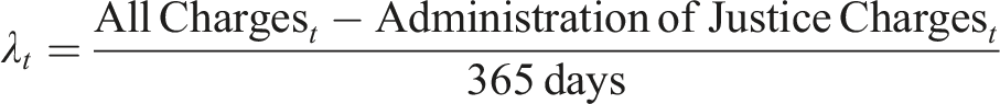
λ_{t} = \frac{{All Charges}_{t} - {Administration of Justice Charges}_{t}}{365 days}

We exclude administration of justice offences from the number of charges to match the data on open caseload. The exclusion of these charges ensures that administration of justice offences, which are often related to other offences, are not double-counted in the data. For cases disposed of in year t with duration longer than a year, it is assumed that the case began, or “arrived”, in the previous year and is thus accounted for in the previous year’s count of all charges arriving in year t − 1. This assumption is made for simplicity. In practice, our estimates do not vary much when we change the arrival date of cases exceeding one year and our data are censored at cases exceeding one year in length. For that reason, data from the final year in the sample, 2018/2019, is omitted from calculations involving the arrival rate λ_t in the paper, as charges that were laid, or “arrived”, in 2019 and lasted longer than one year are unreported in the data, as they are completed in 2019/2020. 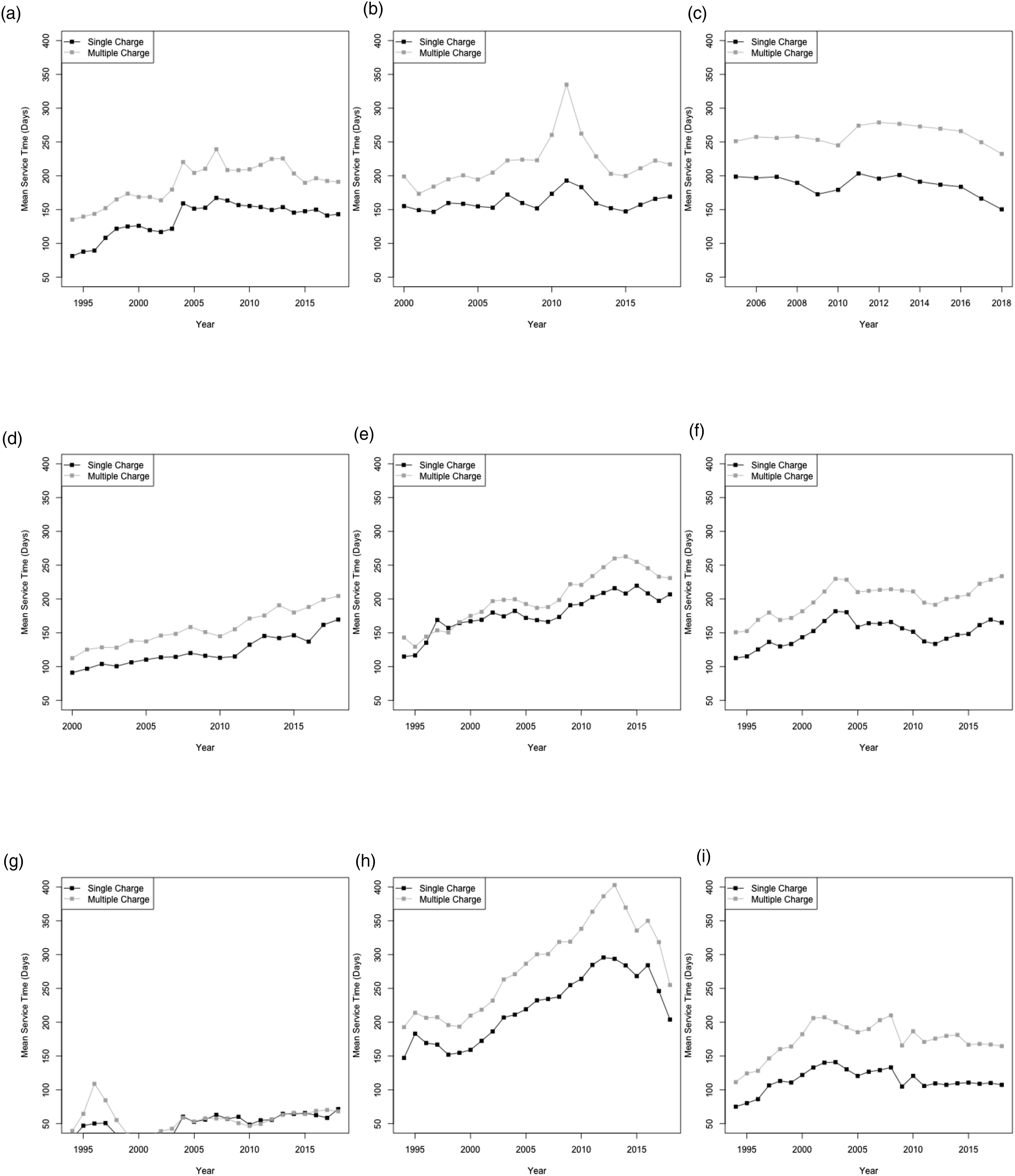Values of the estimated yearly arrival rate λ_t are plotted separately for single and multiple charges are plotted in Figure 4. It can be seen quite easily from Figure 4 that the arrival rate for 2018–2019 criminal charges are plausibly underestimated due to charges that were carried into the following year.

Figure 4.

Mean arrivals per day λ_t. (a) Alberta, (b) British Columbia, (c) Manitoba, (d) New Brunswick, (e) Nova Scotia, (f) Ontario, (g) Prince Edward Island, (h) Quebec, (i) Saskatchewan.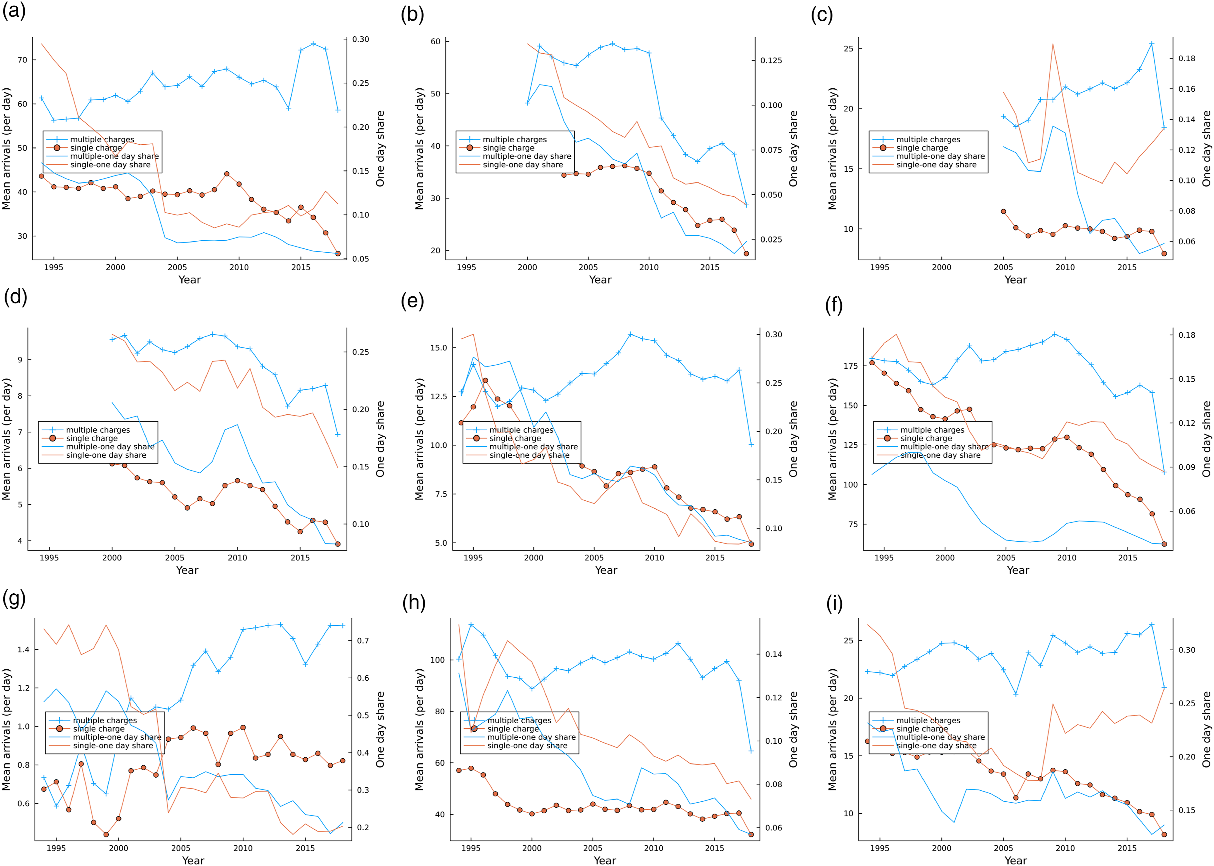

Figure 4 also plots the share of cases that have a service time of one day. The fraction of cases for which the court is able to produce a verdict in one day is extremely large relative to the theoretical probability implied by the duration of the case – one day – under most continuous probability distributions. Appendix A reports the fraction of cases with a duration of one day by offence and year for Alberta, Ontario, and Quebec. At one point in time, the one day case was most likely to be a prostitution or drug possession charge, but increasingly it has become used for crimes related to the administration of justice, such as failure to comply or failure to appear. Guilty pleas or dismissal or withdrawal of charges likely explain these quick, one-day cases. Indeed, in Canada around ninety percent of cases are resolved through the acceptance of guilty pleas (Statistics Canada, 2004).

2.5. Validating the Charge-Level Arrival Rate

The central reason we prefer our construction of the arrival rate from ICSS data is because it is available over a longer time series, going back to 1994 for most provinces. The two data, the ICCS and the CWI, are constructed differently in important ways: in the CWI, a case that is initiated is defined in terms of the information, which contains all charges per information, while the ICCS data, though more readily available over a longer series, provide data on the total number of charges with no information on the number of charges per information. However, we can validate our measure of the arrival rate by comparing it with the workload measure of cases initiated in a given year.

Figure 5 plots the relationship between our measure of arrivals and the cases initiated in a given year for the sub-sample for which we have both measures of arrivals. We find a robust positive relationship both in from regressions in logs and levels of the number of charges laid in a given year according to our measure on the number of cases initiated in that same year. Indeed, the correlation coefficient between the two measures of arrivals is 0.99. However, the coefficient estimate on the levels regression indicates that the arrival rate we construct under-estimates the total number of cases arriving in a given year, as the coefficient is below one, contrary to what one might expect if there were double-counting of charges per information in the ICCS data. This suggests the double-counting problem with cases of multiple-charges per information is not as severe as one might expect. Nevertheless, the high Pearson’s correlation and log coefficient of approximately one suggest that the ICCS measure of arrivals is appropriate to extrapolate the mean daily arrivals back in time with ICCS data, which we have beginning in 1994 for most provinces.

Figure 5.

Relationship between cases initiated and mean daily arrivals. Note. Figure plots number of charges in a given year (excluding administration of justice offences) (Source: Integrated Criminal Court Survey (ICCS)). Against the total number of cases initiated in a given year (Source: Court Workload Indicators). Coefficients are from regressions, both in levels and in logs, of the number of arrivals on the number of cases initiated. Correlation is Pearson’s correlation coefficient.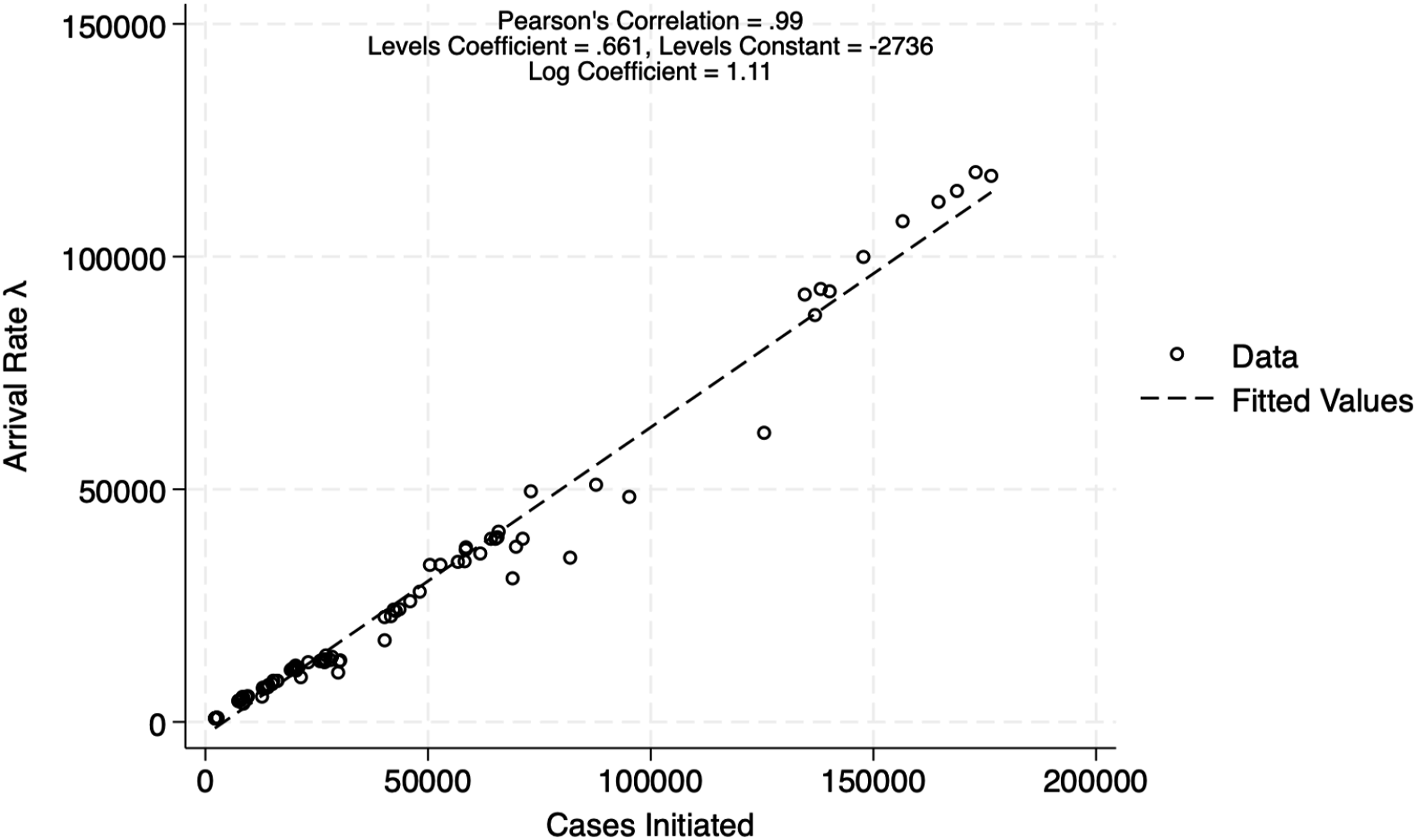

3. Estimation of Service Rate

Our goal in this section is to identify probability distributions that are consistent with our trial duration data, and use those distributions to obtain parametric estimates of mean trial duration. The service rate is defined as the time from first appearance to final disposition, or the end of trial, were there to be one. These estimates are, in turn, critical inputs into our estimates of pre-trial waiting times, as discussed later in Section 4.

It is important to note that our data is zero-inflated in the sense that far more trials are resolved extremely quickly (i.e., in less than one day) than would be implied by any of the most familiar probability distributions. To illustrate we consider the province of Ontario in 2010, in which case 11% of all single-charge cases required more than one year to resolve. If we were to assume that trial durations (as measured in days) followed an exponential distribution with rate β, then in order to match this observed frequency we would require 0.11 = e^−365β or β ≈ 0.006. Now, if trial durations were exponentially distributed with rate β = 0.006 then the probability an individual trial is resolved within one day is 1 − e^−0.006 ≈ 0.006 and we should expect to see 0.6% of all trials resolved within one day. In fact, for Ontario in 2010, 12% of all single-charge cases were resolved within one day, twenty times the rate implied by the exponential distribution as fit to the year-long trials. The point here is simple: the exponential distribution is unable to account for the substantial number of trials that are resolved extremely quickly, while simultaneously providing a good fit to the remaining data (i.e. durations of trials that are not resolved extremely quickly). One finds the same issue with virtually any of the most common probability distributions.

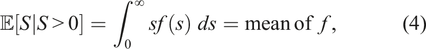
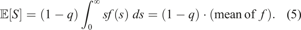
In order to formally describe our approach, let the random variable S denote the duration of an arbitrary trial in a given jurisdiction and year. We assume there is a positive probability that S = 0 and that if S > 0, then S behaves as a continuous random variable. In other words, we assume that trial durations are non-negative and continuous random variables, with a point mass at zero (the point mass being necessary to account for the substantial proportion of cases that are resolved extremely quickly). Formally, we assume that there exists a number q ∈ [0, 1] and probability density function f, supported on [0, ∞), such that

P (S = 0) = q and P (a < S < b | S > 0) = \int_{a}^{b} f (s) d s

for any 0 < a < b. For example if q = 0.10 and f(s) = 0.01e^−0.01s then P(S = 0) = 0.1 and the conditional distribution of S, given that S > 0, is exponential with a mean of 100 days. Note that we allow both f and q to vary across year, province and case type (single- or multiple-charge).

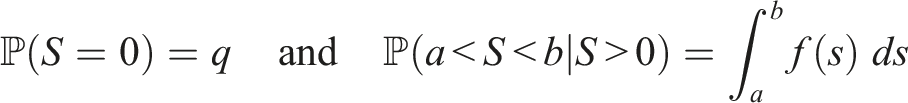
For later use, we note that for any 0 < a < b we have

P (S \leq a) = q + (1 - q) F (a),

(1)

P (S \geq b) = (1 - q) [1 - F (b)]

(2)

and

P (a \leq S \leq b) = (1 - q) [F (b) - F (a)],

(3)

where

F (s) = \int_{0}^{s} f (u) d u

is the cumulative distribution function (cdf) of f. In addition, it is straightforward to verify that the average duration of trials that are not resolved extremely quickly is

E [S | S > 0] = \int_{0}^{\infty} s f (s) d s = mean of f,

(4)

whereas the average duration of all trials (including those that are resolved extremely quickly) is

E [S] = (1 - q) \int_{0}^{\infty} s f (s) d s = (1 - q) \cdot (mean of f) .

(5)

3.1. Parametric Estimates

It is tempting to assume that trial durations are exponentially distributed; queueing models with memoryless¹⁴ service times tend to be the most mathematically tractable. That being said it is important to consider potential departures from memorylessness, and to this end we consider two different parametric families. A random variable is said to have a Weibull (Extreme Value Type III) distribution with scale parameter β > 0 and shape parameter α > 0 if it has a probability density function (pdf) of the form

f (s) = (α β) {(β s)}^{α - 1} e^{- {(β s)}^{α}} .

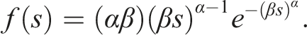
The Weibull mean is βΓ(1 + α⁻¹), where Γ(⋅) denotes the gamma function, and the Weibull hazard fuction is

h (s) = (α β) {(β s)}^{α - 1}

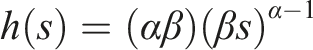
Note that if α = 1 then the Weibull distribution reduces to the exponential. If α > 1 then the hazard function is increasing and there is a negative relationship between a trial’s current age (number of days since it began) and remaining lifetime (expected time until resolution); the opposite is true if α < 1. If α = 1 then the hazard function is constant and the memoryless property prevails. Presumably the case α > 1 is more desirable in the present context, although that is admittedly a judgment call. An estimated value of α that is close to one would suggest that the memoryless property is a reasonable assumption for trial durations; an estimate that deviates substantially would indicate that the memoryless assumption is questionable.

It is also important to assess whether or not trial durations have so-called “heavy tails”, in which case excessively long trials would occur with concerning frequently. To this end we also consider the lognormal family, and recall that the random variable S is said to have a lognormal distribution with location parameter $m \in R$ and scale parameter v > 0 if ln(S) follows a normal distribution with mean m and standard deviation v.

In what follows we let θ denote the vector of unknown parameters in a given family, that is θ = β for the exponential, θ = (α, β) for the Weibull and θ = (m, v) for the lognormal. We write f(s; θ) and F(s; θ) instead of f(s) and F(s) in order to emphasize that the pdf and cdf do depend on the specific values of the parameters parameters (i.e., different parameter values produce different pdfs and cdfs).

We assume that within a given year, province and class (single- or multiple-charge), trial durations are independent and identically distributed. Unfortunately, we do not have access to exact trial durations, rather we have access to binned count data. In particular, for each year and province we have access to the number of trials whose ultimate durations were (i) less than one day, (ii) between 1 and 61 days, (iii) between 61 and 121 days, (iv) between 121 and 241 days, (v) between 241 and 365 days and (vi) in excess of one year. In other words our observed data is a vector of counts (n₁, n₂, n₃, n₄, n₅, n₆) where n_i is the number of observations in the i^th bin (e.g., n₂ is the number of trials whose ultimate durations were between 1 and 61 days).

3.2. Parameter Estimation

The log-likelihood function that we are faced with is demonstrably given by

ℓ (q, θ) = C + n_{1} \log (q + (1 - q) p_{1} (θ)) + (n - n_{1}) \log (1 - q) + \sum_{i = 2}^{6} n_{i} \log (p_{i} (θ)),

(6)

where C is a constant that depends on the n_i but not on q or θ,

n = \sum_{i = 1}^{6} n_{i}

, p₁(θ) = F(1; θ) − F(0; θ), p₂(θ) = F(61; θ) − F(1; θ), …, p₆(θ) = 1 − F(365; θ). In general (6) must be maximized numerically, which is straightforward using most mathematical software.¹⁵ In what follows we let

\hat{q}

and

\hat{θ}

denote the resulting (and numerically obtained) maximum likelihood estimates. As it turns out

p_{1} (\hat{θ}) \approx 0

in all cases (years, provinces and case types), which means that future researchers may wish to use the simpler log-likelihood function

ℓ (q, θ) = C + n_{1} \log (q) + (n - n_{1}) \log (1 - q) + \sum_{i = 2}^{6} n_{i} \log (p_{i} (θ)) .

(7)

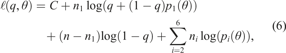
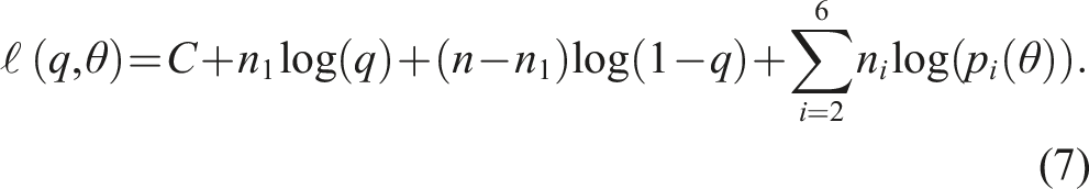
The advantage of (7) is that q and θ can be estimated separately. Indeed $\hat{q} = n_{1} / n$ can be computed in closed form and $\hat{θ}$ can be obtained by numerically maximizing the lower-dimensional function $\sum_{i = 2}^{6} n_{i} \log (p_{i} (θ))$ .

3.3. Model Selection

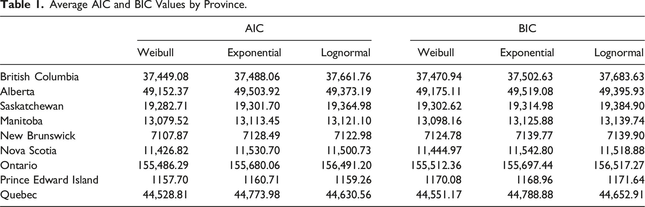
In this section we attempt to determine which of our three parametric models best fits the trial duration data. We begin by computing, for each year and province, the Akaike information criterion (AIC) and Bayesian information criterion (BIC) for each model. Recall that the AIC value for a particular model (in a particular year and province) is $2 k - 2 ℓ (\hat{θ})$ , where k is the number of parameters in the model, whereas the BIC value is $k \ln (n) - 2 ℓ (\hat{θ})$ . When faced with competing models, the best fitting model is typically taken to be that model with the smallest AIC and/or BIC value. Note also that each criteria balances model fit (as measured by likelihood) and complexity (number of parameters).

Table 1 reports the average (across years) AIC and BIC values for each province. Perhaps the clearest signals from the table are that (i) the data does not suggest that trial durations are heavy tailed, and (ii) the Weibull family is more often preferred (by these criteria) across provinces. The mean service times are relatively similar under the various distributional assumptions. The p values give us a sense of whether the discrepancy between the distributions is large or small.

Table 1.

Average AIC and BIC Values by Province.

	AIC			BIC
	Weibull	Exponential	Lognormal	Weibull	Exponential	Lognormal
British Columbia	37,449.08	37,488.06	37,661.76	37,470.94	37,502.63	37,683.63
Alberta	49,152.37	49,503.92	49,373.19	49,175.11	49,519.08	49,395.93
Saskatchewan	19,282.71	19,301.70	19,364.98	19,302.62	19,314.98	19,384.90
Manitoba	13,079.52	13,113.45	13,121.10	13,098.16	13,125.88	13,139.74
New Brunswick	7107.87	7128.49	7122.98	7124.78	7139.77	7139.90
Nova Scotia	11,426.82	11,530.70	11,500.73	11,444.97	11,542.80	11,518.88
Ontario	155,486.29	155,680.06	156,491.20	155,512.36	155,697.44	156,517.27
Prince Edward Island	1157.70	1160.71	1159.26	1170.08	1168.96	1171.64
Quebec	44,528.81	44,773.98	44,630.56	44,551.17	44,788.88	44,652.91

Table 1 suggests that the Weibull family provides a better fit to the data than either the exponential or lognormal families, but that does not necessarily mean it provides a good fit. To this end we use the Pearson’s χ² test to formally test the null hypothesis that the data was drawn from a Weibull distribution, against the broad alternative that it was not drawn from a Weibull. For completeness we conduct the same test for each of the other two families. For each province we perform separate tests in each year, and the first three columns of Table 2 report average (across years) p values. The results reported in the table suggest that the Weibull does fit the data well in nearly every province, whereas the lognormal family is soundly rejected in all but one province. Of particular interest is the fact that the exponential family also provides a good fit across half the provinces.

Table 2.

Average p Values by Province.

	Pearson χ₂			Likelihood Ratio
	H₀: Weibull	H₀: Exponential	H₀: Lognormal	H₀: Exponential
	H_a: Not Weibull	H_a: Not Exponential	H_a: Not Lognormal	H_a: Weibull
British Columbia	0.53	0.13	0.00	0.04
Alberta	0.02	0.00	0.03	0.00
Saskatchewan	0.89	0.51	0.03	0.12
Manitoba	0.91	0.35	0.24	0.02
New Brunswick	0.75	0.37	0.41	0.06
Nova Scotia	0.85	0.09	0.08	0.00
Ontario	0.13	0.06	0.00	0.08
Prince Edward Island	0.99	0.96	0.97	0.32
Quebec	0.50	0.00	0.01	0.00

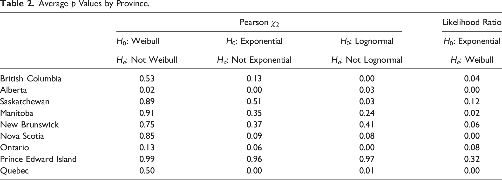
Because the Weibull contains the exponential as a special case, it is possible to directly test the hypothesis that trial durations are memoryless. To this end we assume the data is drawn from a Weibull distribution and employ a likelihood ratio test to test the null hypothesis that α = 1 (memoryless) against the alternative that α ≠ 1 (not memoryless). The last column of Table 2 reports average p values for each province. The data does cast some doubt on the validity of the memoryless assumption, but the evidence is certainly not overwhelming across all provinces.

3.4. Results

The first column of Table 3 reports estimated mean trial durations obtained from the Weibull distribution. Recall that our ultimate goal here was parametric estimates of mean trial durations. For each year we estimate the model parameters

(\hat{q}, \hat{θ})

, compute the mean trial duration via

(1 - \hat{q}) Γ (1 + {\hat{α}}^{- 1}) {\hat{β}}^{- 1}

and report the average of these values in the table. Our estimates imply that service times are on the order of months in each province. It is worth noting that estimates obtained from the exponential distribution are quite comparable to those obtained from the Weibull distribution (typically differing only by a few days, which is unsurprising in light of how close the Weibull shape parameters are to unity, the case in which the Weibull distribution nests the exponential distribution.

Table 3.

Weibull Mean Service Time Estimates.

Province	Duration	Shape Parameter	Trend (Days/Year)	p Value
Alberta	168	1.1	2.94	0
British Columbia	195	0.97	1.69	0.109
Manitoba	235	1.09	−0.14	0.87
New Brunswick	144	1.11	4.27	0
Newfoundland and Labrador	161	1.16	6.93	0
Nova Scotia	192	1.18	4.51	0
Ontario	179	1.01	2.18	0
Prince Edward Island	52	0.97	1.06	0.007
Quebec	263	1.11	6.89	0
Saskatchewan	150	1	1.24	0.04

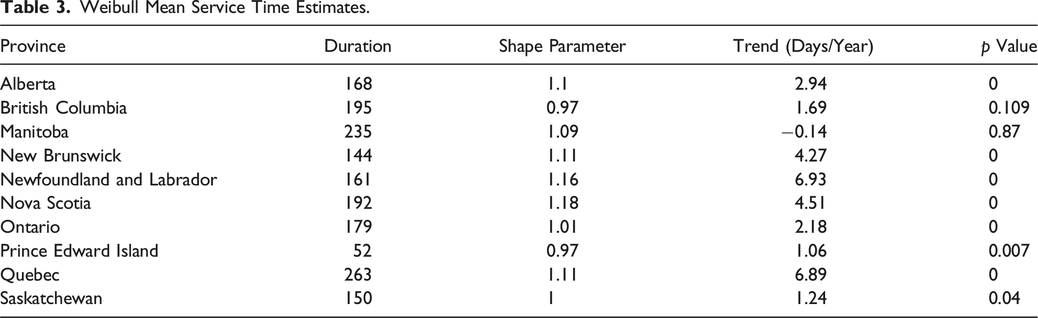
The second column of Table 3 displays the average estimated Weibull shape parameter across provinces. For each province we estimate a separate value of $\hat{α}$ for each year, and report the average of these values in the table. Most estimates exceed one, which appears to be a positive sign (recall that if the shape parameter exceeds one then the hazard function is increasing). Our estimates are also close to one (extremely close, in some cases), which suggests that the memoryless assumption might be innocuous. In other words, we have strong statistical evidence that the Weibull shape parameter is marginally different from one (i.e., the data strongly suggests a marginal departure from the exponential distribution, and thereby memorylessness). The distribution of the shape parameter from the Weibull estimates across years for each province are displayed in Figure 6. In all models, given our large sample size, all parameter estimates will be statistically significant.

Figure 6.

Weibull Shape Parameters α from CDF 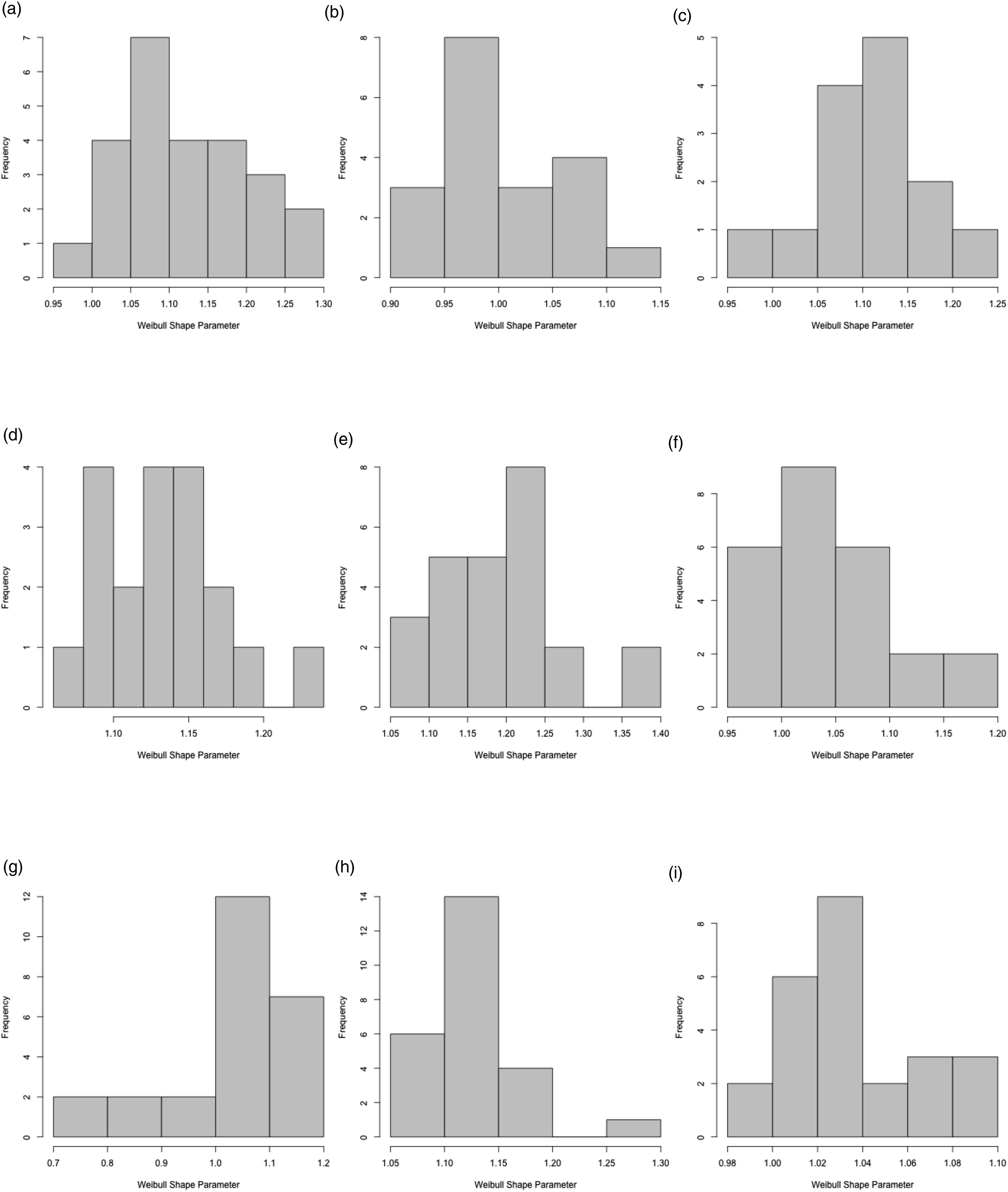$F (x) = 1 - \exp (- {(β x)}^{α})$ . (a) Alberta, (b) British Columbia, (c) Manitoba, (d) New Brunswick, (e) Nova Scotia, (f) Ontario, (g) Prince Edward Island, (h) Quebec, (i) Saskatchewan.

The last two columns of Table 3 consider time trends in mean trial durations. Specifically, for each province we regress our estimated mean durations against a time variable. The third row of the table reports estimated coefficients and the fourth row reports the p value associated with the test of the null hypothesis that the coefficient is equal to zero. In all but one or two provinces the estimated time trend coefficient is positive and statistically significant.

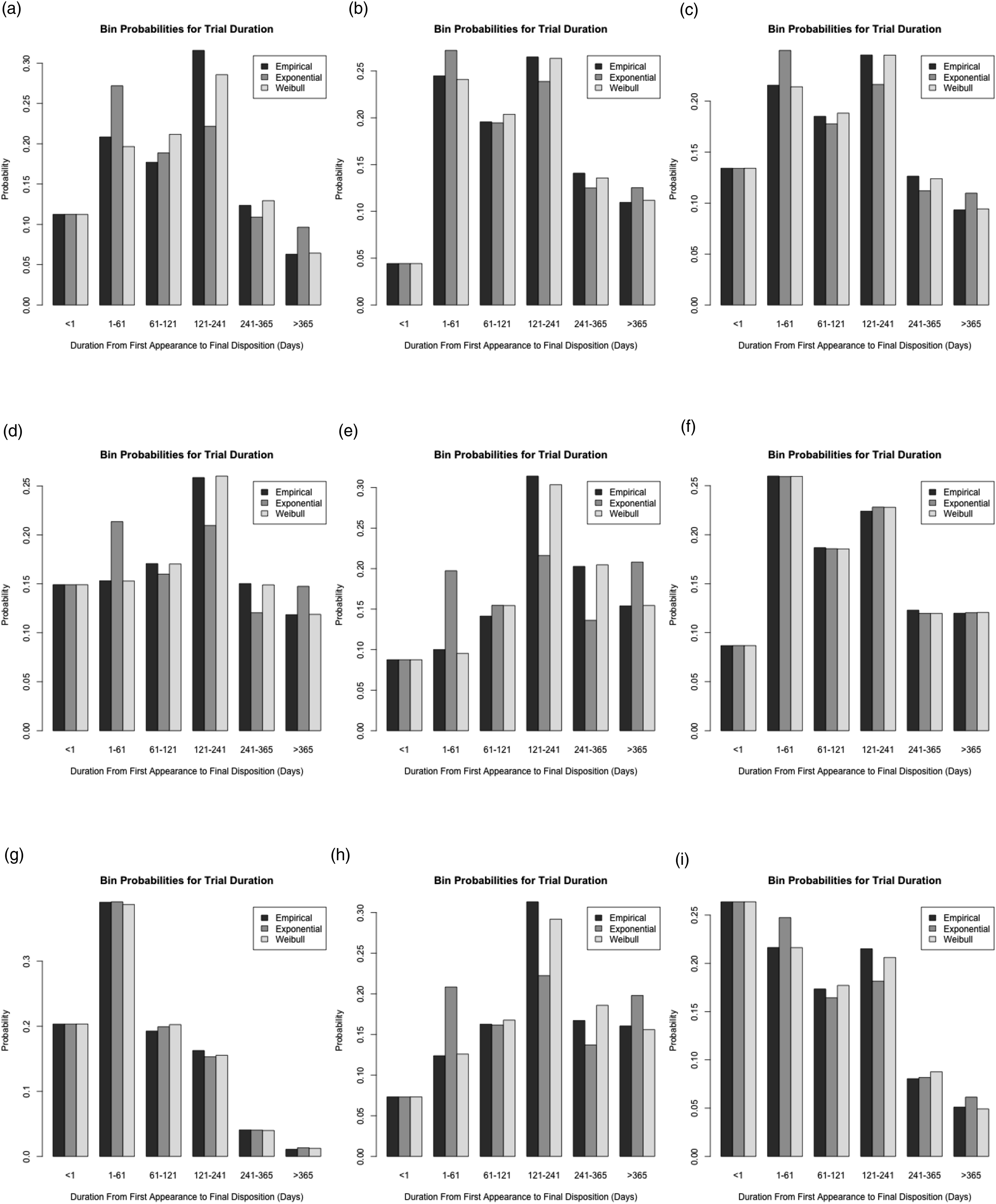
The results from the maximum likelihood procedure estimating the rate of the empirical service time distribution are displayed in Figure 7. It is important to remember that for the exponential distribution the mean is always greater than the median since ln(2) < 1, meaning that over half of cases will be served below the mean service time. The figure plots the mean of the Weibull distribution

μ^{* - 1} = \frac{1 - q}{β} Γ (1 + α^{- 1})

(8)

where β is the estimate from the maximum likelihood procedure on case durations. To get a sense of how well the theoretical exponential distributions fit the data, Figure 8 plots the empirical probabilities against the theoretical proportions from the MLE procedure for 2018–2019 across provinces. Overall, we can conclude that the empirical distribution follows the theoretical exponential distribution quite closely, suggesting a good fit.

Figure 7.

Mean service time: Inverse of maximum likelihood estimates $μ_{t}^{* - 1}$ : 1994–2019. (a) Alberta, (b) British Columbia, (c) Manitoba, (d) New Brunswick, (e) Nova Scotia, (f) Ontario, (g) Prince Edward Island, (h) Quebec, (i) Saskatchewan.

Figure 8.

Empirical versus Theoretical Service Time Distributions: 2018–2019. (a) Alberta, (b) British Columbia, (c) Manitoba, (d) New Brunswick, (e) Nova Scotia, (f) Ontario, (g) Prince Edward Island, (h) Quebec, (i) Saskatchewan.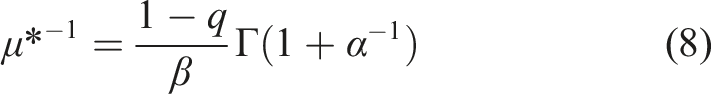

3.5. Grouped Charges

For the multiple charge data we can no longer consider the n_i as “true” bin counts. Indeed the duration of a trial considering, say, three charges would be triple-counted in (6). The implication is that estimates based on (6) could potentially be skewed by the realized durations of larger trials (larger trials meaning those that consider more charges). In this section we argue that if there is no statistical relationship between trial size (number of charges being considered in that trial) and trial duration, then parameter estimates based on (6) should be reasonably accurate. While it is conceivable that there is a relationship between duration and number of charges, we do not have access to any information on trial size so it is not possible for us to assess whether such a relationship exists.¹⁶ That being said, and as we discuss in this section, if duration and size are statistically independent then our estimation procedure for the single-charge data continues to be valid upon the inclusion of multiple-charge cases.

To begin suppose that the n charges are grouped into m cases. For 1 ≤ j ≤ m let S_j denote the realized duration of the j^th case, and for 1 ≤ i ≤ 6 let m_i denote the number of cases for which S_j falls in bin i. Further suppose we have access to the true bin counts (m₁, m₂, m₃, m₄, m₅, m₆). Then, under the assumption that trial size and duration are statistically independent, the log-likelihood function associated with the true counts is demonstrably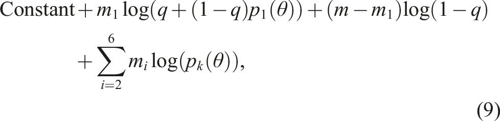

Constant + m_{1} \log (q + (1 - q) p_{1} (θ)) + (m - m_{1}) \log (1 - q) + \sum_{i = 2}^{6} m_{i} \log (p_{k} (θ)),

(9)

where the constant does not depend on q or θ, and where

m = \sum_{i = 1}^{6} m_{i}

In order to compare the likelihood functions (9) and (6) we proceed as follows. For 1 ≤ i ≤ 6 and 1 ≤ ℓ ≤ m_i let c_ℓ,i denote the number of charges associated with the ℓ^th case, among those cases for which the realized trial duration fell in bin i. Finally, let 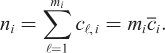${\bar{c}}_{i} = 1 / m_{i} \sum_{ℓ = 1}^{m_{i}} c_{ℓ, i}$ denote the average number of charges per trial, among those trials whose durations belong to bin i, and note that

n_{i} = \sum_{ℓ = 1}^{m_{i}} c_{ℓ, i} = m_{i} {\bar{c}}_{i} .

Now, if trial size and duration are independent, and we have a large number of observations, we would expect that the 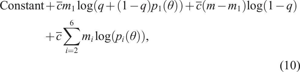${\bar{c}}_{i} \approx \bar{c}$ for every i, where $\bar{c}$ is the overall average number of cases per trial. In this case (6) reduces to

Constant + \bar{c} m_{1} \log (q + (1 - q) p_{1} (θ)) + \bar{c} (m - m_{1}) \log (1 - q) + \bar{c} \sum_{i = 2}^{6} m_{i} \log (p_{i} (θ)),

(10)

and it is clear that the same values of (q, θ) that maximize (9) will maximize (10) and therefore (6). Thus, if duration and size are statistically independent, our single-charge estimation procedure should also be appropriate in the multiple-charge setting. However, we derive an approach for using charge-level data for future researchers who have data on the number of charges per information and whether a trial undergoes a preliminary inquiry.

4. Queueing Theory

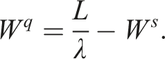
We now use our data and estimates to construct a model of the criminal justice system in each year for each province. Throughout our analysis, we are using long-run, equilibrium relationships assuming that one year is long enough for those relationships to materialize, as queueing theory uses expectations to model the average behaviour of a system over time. To measure the total number of cases in the system, L_t, we use data on the provincial court system’s open caseload. With our arrival rate λ_t, we can use Little’s Law (Little, 1961) to calculate total time in the system, and then subtract average service time 1/μ* to obtain the average implied wait time. Finally, we construct an estimate of the queue size L^q by subtracting our estimate of the system’s server-level utilization rate ρ_t = λ_t/μ_t from the total number in the system L_t.¹⁷

We exploit Little’s Law, an important queueing identity that applies to an extremely wide class of queueing models. Under extremely mild assumptions, Little’s Law states that

L = λ W

where L is the average number of customers in the system, both waiting in the queue and currently being served, λ is the arrival rate and W is the average amount of time customers spend in the system, both waiting for service and and the duration of service itself. Because of its generality, Little’s Law allows us to estimate the average amount of time individuals spend in the court system without having to impose strong assumptions on the underlying structure of the model. It will always be the case that W = W^q + W^s, where W^q is the amount of time the average customer spends waiting for service (in queue) and W^s is the amount of time the average customer spends being served. Inserting this identity into Little’s Law and re-arranging allows us to express the average waiting time as

W^{q} = \frac{L}{λ} - W^{s} .

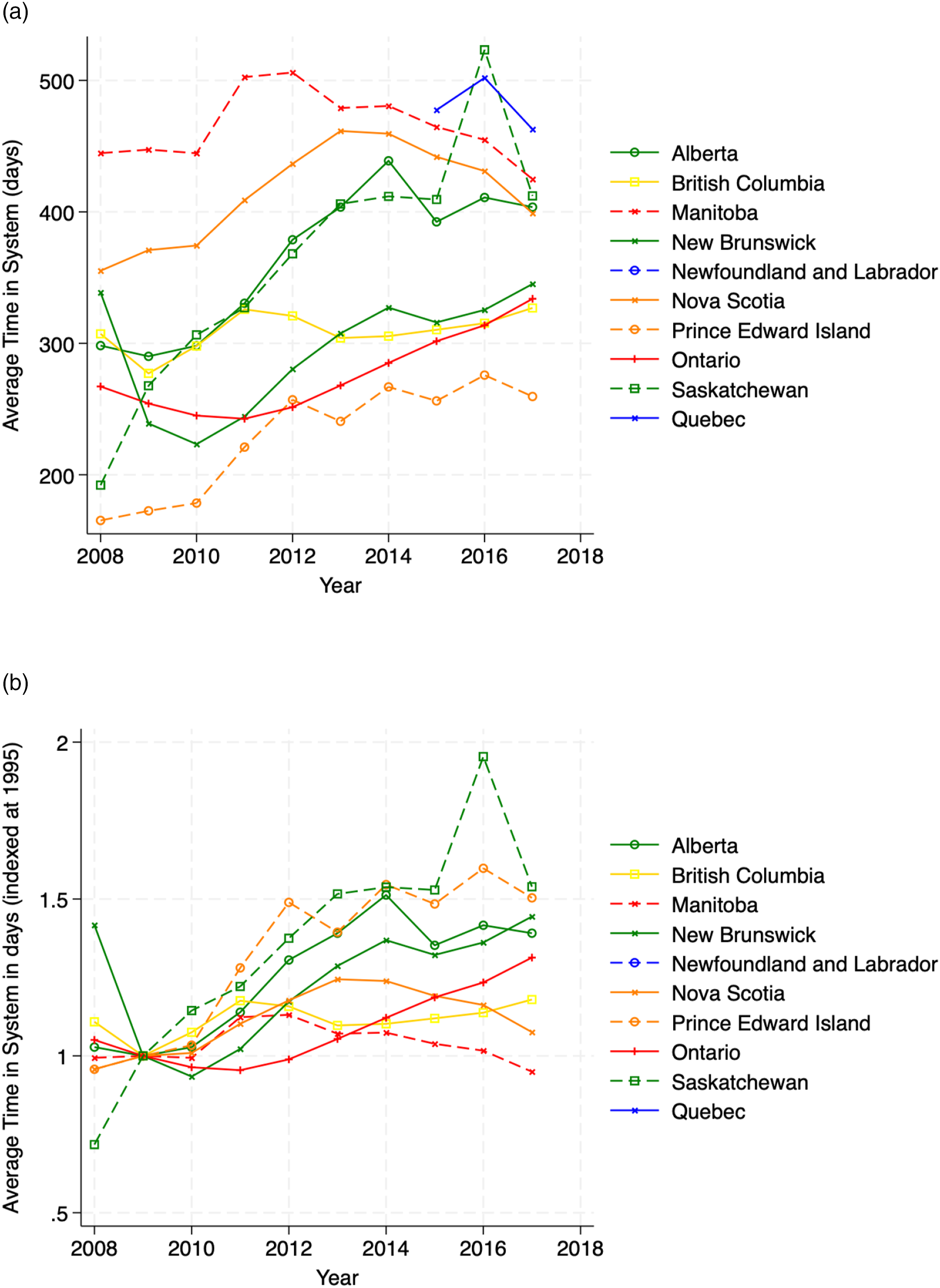
Armed with estimates of the arrival λ_t and service rates μ_t, as well as estimate of the average number of open cases during a given year L_t, we can extract estimates of average waiting times in a particular year:

W_{t}^{q} = \frac{L_{t}}{λ_{t}} - \frac{1}{μ_{t}}

(11)

where L_t, λ_t and μ_t are the average open caseload, estimated arrival rate, and estimated service rate in year t, respectively. Total time in the system W and wait time W^q are in Figures 9 and 10. In general, both time in system and wait times are increasing across our series. The time to trial has grown fastest in Saskatchewan, where the implied average time to first appearance has risen to approximately three hundred days. However, wait times have also risen by a factor of nearly two in Ontario and British Columbia, where we estimate wait times to be the shortest.

Figure 9.

Implied time in system W. (a) Implied time in system $W t = \frac{L_{t}}{λ_{t}}$ ., (b) implied time in system W_t indexed at 2009.

Figure 10.

Implied time in Queue W^q. (a) Implied time in Queue 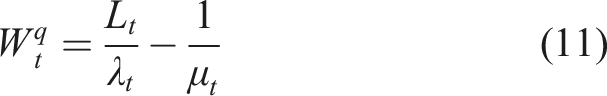$W_{t}^{q} = \frac{L_{t}}{λ_{t}} - μ_{t}^{- 1}$ , (b) implied time in Queue $W_{t}^{q}$ indexed at 2009.

Regardless of the exact specification, many important measures of congestion, such as average time in system, average time in line, number of customers waiting for service, depend, in an increasing way, on the utilization rate – the ratio of the arrival rate λ_t to the service rate μ_t. In our notation, the utilization rate ρ_t in year t would be

ρ_{t} = \frac{λ_{t}}{μ_{t}}

where we recall that μ⁻¹ = (1 − q)/β is the mean service time and β is the exponential rate fit to the

> 1

day data. Queueing theory suggests that an increase in the utilization rate is a strong signal that the system is experiencing higher traffic, and that, in the absence of interventions, wait times could grow rapidly.¹⁸ Time-varying utilization rates are plotted for each province in Figure 11. The server-level utilization rates are in the several thousands. In a multiple-server queueing model, the utilization rate as defined in equation above is equal to the number currently being served, assuming the number of servers exceeds the system-level utilization rate λ/cμ < 1 ⇒ ρ < c.¹⁹

Figure 11.

Utilization rates $ρ_{t} = λ_{t} / μ_{t}^{*}$ . (a) Alberta, (b) British Columbia, (c) Manitoba, (d) New Brunswick, (e) Nova Scotia, (f) Ontario, (g) Prince Edward Island, (h) Quebec, (i) Saskatchewan.

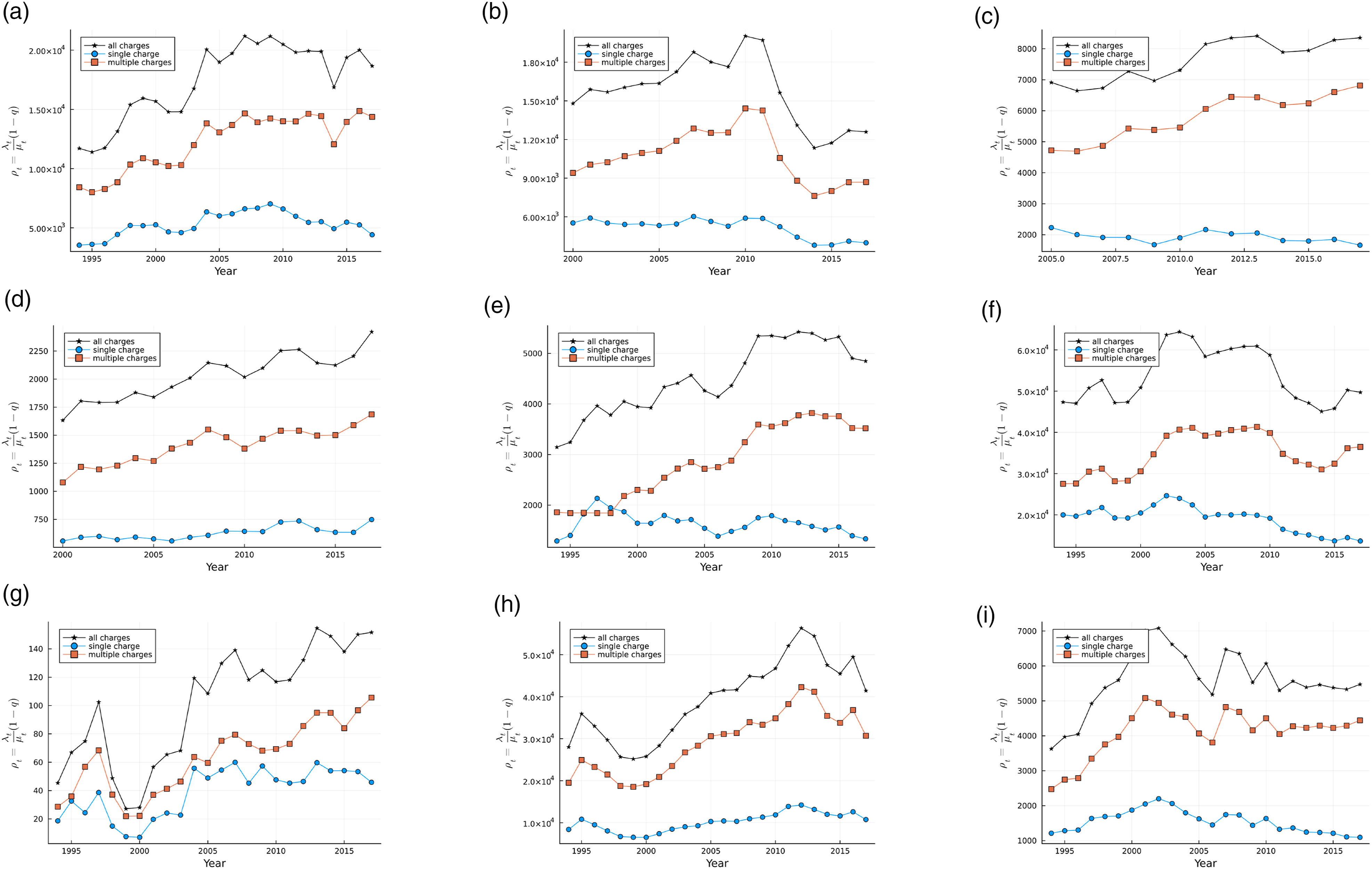
We use data on the open caseload at any given point in time to measure the total number in the system, both in the queue and being served, which we denote as L_t. The total number in the system L_t and the number being served ρ_t are plotted in Figure 12. Indeed, we find that queueing theory’s measure of the number being served ρ_t is highly correlated with open caseload, the total number in the system L_t, suggesting that queueing theory has explanatory power. However, as we shall see, with a finite number of servers, the difference between these two quantities is the size of the queue.

Figure 12.

Open caseload L_t and Utilization ρ_t. Note. Figure plots open caseload L_t and the server-level utilization rate ρ_t. (a) Alberta, (b) British Columbia, (c) Manitoba, (d) New Brunswick, (e) Nova Scotia, (f) Ontario, (g) Prince Edward Island, (h) Quebec, (i) Saskatchewan.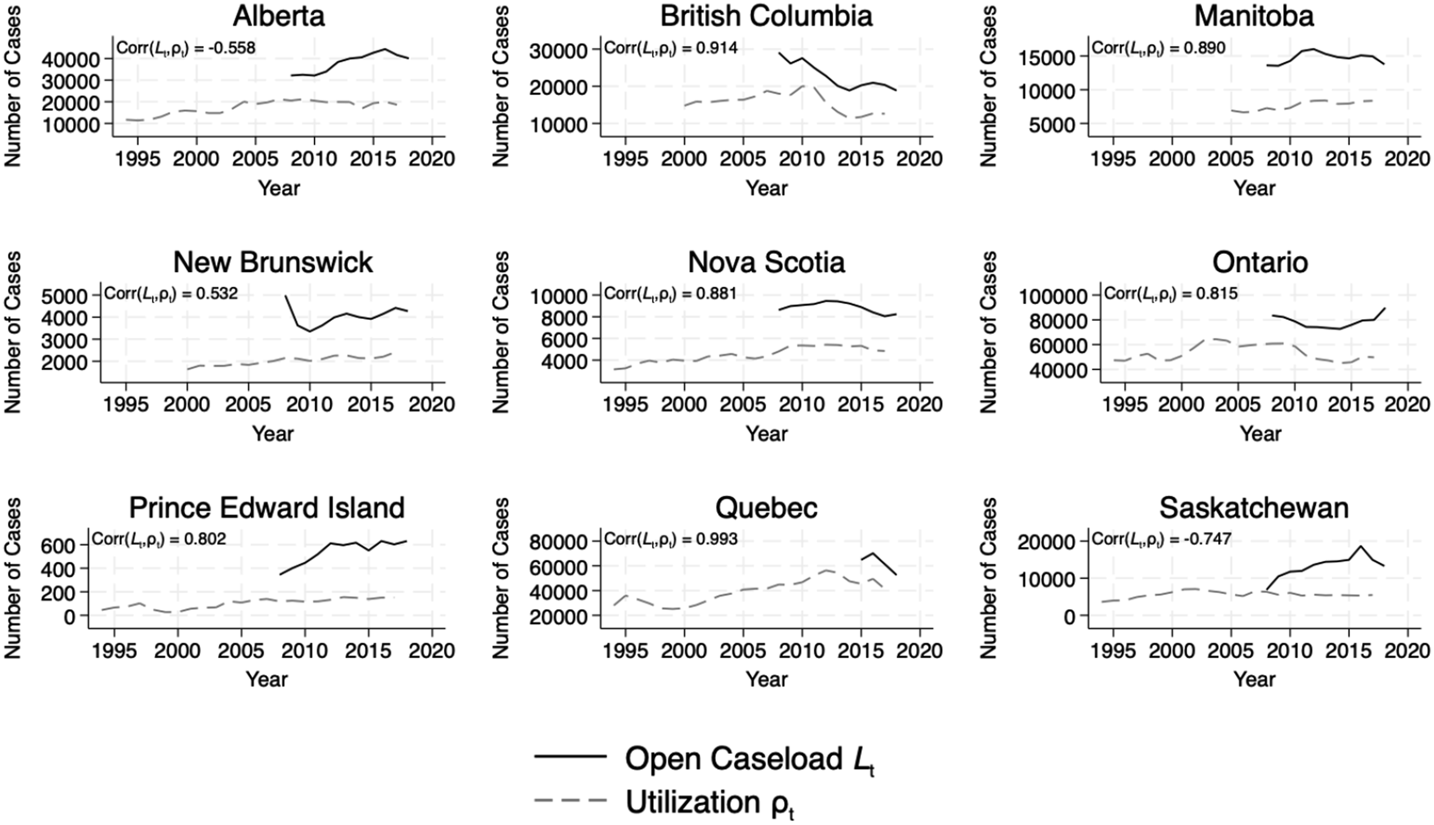

The queue size L^q can be backed out again using Little’s Law for queues

L^{q} = λ W^{q} .

Inserting the equation for W^q yields

L_{t}^{q} = L_{t} - \frac{λ_{t}}{μ_{t}}

(12)

where we have estimated L_t using data on the court system’s open caseload and λ_t and μ_t is estimated via MLE. The implied queue size from a steady-state system are plotted in Figure 13(a) and indexed at 2009 in Figure 13(b).

Figure 13.

Implied number in Queue L^q. (a) Implied number in Queue 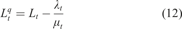$L_{t}^{q} = L_{t} - \frac{λ_{t}}{μ_{t}}$ , (b) Implied Number in Queue $L_{t}^{q}$ Indexed at 2009.

4.1. Stationarity

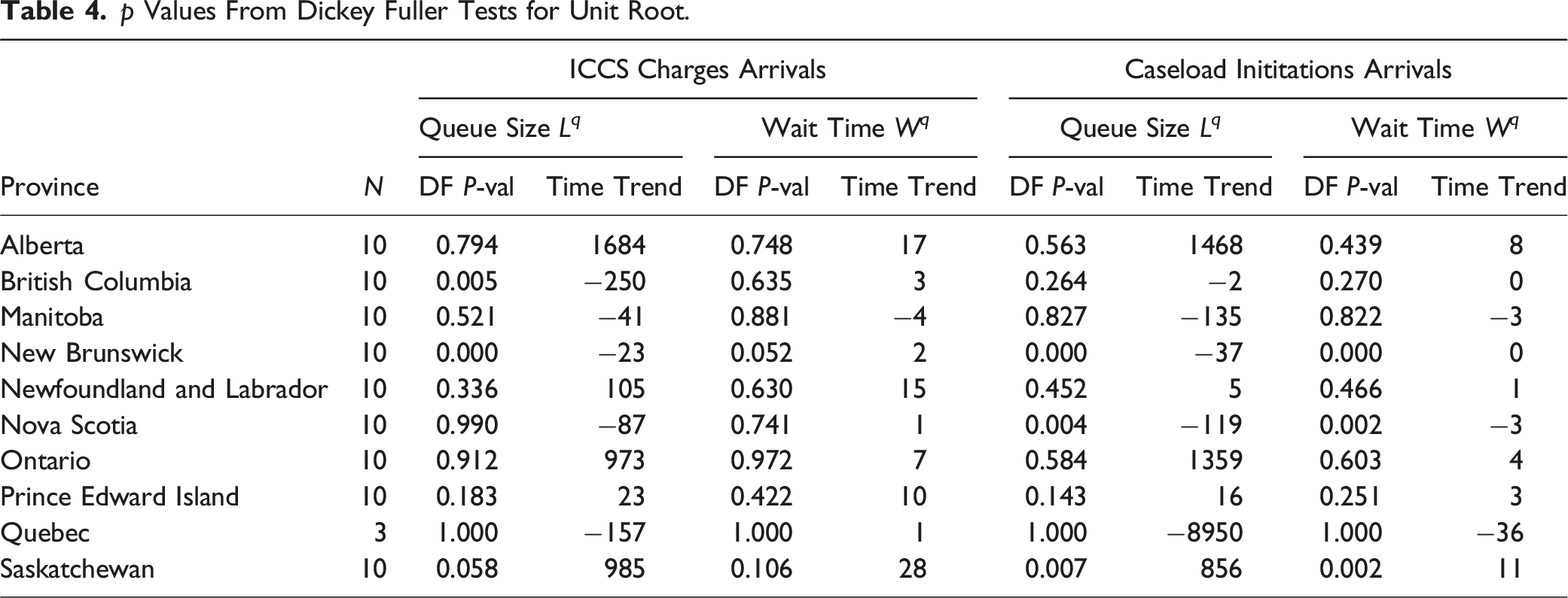
Table 4 displays the p values from a test for a unit root (non-stationarity) in the queueing series using the augmented Dickey-Fuller test. The p values are well above the five percent cutoff, failing to reject the null hypothesis of a unit root, suggesting that the queue and wait time behaviour are non-stationary across many provinces. Indeed, using both ICCS charge data and cases initiated produces queue and wait times which we fail to reject as having a unit root. The table also reports the coefficient from the regression of the wait time or queue size on a year variable (i.e., a time trend). The results suggest that the wait times and queue size are growing in many provinces that do not have a unit root.

Table 4.

p Values From Dickey Fuller Tests for Unit Root.

Province	N	ICCS Charges Arrivals				Caseload Inititations Arrivals
		Queue Size L^q		Wait Time W^q		Queue Size L^q		Wait Time W^q
		DF P-val	Time Trend	DF P-val	Time Trend	DF P-val	Time Trend	DF P-val	Time Trend
Alberta	10	0.794	1684	0.748	17	0.563	1468	0.439	8
British Columbia	10	0.005	−250	0.635	3	0.264	−2	0.270	0
Manitoba	10	0.521	−41	0.881	−4	0.827	−135	0.822	−3
New Brunswick	10	0.000	−23	0.052	2	0.000	−37	0.000	0
Newfoundland and Labrador	10	0.336	105	0.630	15	0.452	5	0.466	1
Nova Scotia	10	0.990	−87	0.741	1	0.004	−119	0.002	−3
Ontario	10	0.912	973	0.972	7	0.584	1359	0.603	4
Prince Edward Island	10	0.183	23	0.422	10	0.143	16	0.251	3
Quebec	3	1.000	−157	1.000	1	1.000	−8950	1.000	−36
Saskatchewan	10	0.058	985	0.106	28	0.007	856	0.002	11

4.2. Robustness Check: Singe-Charge Cases

An inconvenient feature of our arrivals data is that we only have data on the number of charges with no knowledge of the number of charges per information. One may rightly contend that changes in the composition of charges per information may bias our results, if not merely contribute to measurement error. Moreover, it may be of interest whether congestion in the system is driven by multiple-charge offences, which we have already seen have longer trials, but may also be more likely to opt for a preliminary hearing or a jury trial. To overcome these challenges, we thin out the full queueing system to study only single-charge cases to test if they follow a similar trend in wait times. To calculate the single-charge open caseload, we multiply the total open caseload by the fraction of arrivals that contain only a single-charge.

All model inputs and queueing results are re-produced in Figure 14. The wait times implied from the multiple-server queueing framework are, again, non-stationary and increasing. This allows us to conclude that our main results are not driven by changes in the number of charges per information, as the same phenomena are present in the thinned single-charge system. The fraction of open caseload attributable to single-charge cases is growing relative to the single-charge system server-level utilization.

Figure 14.

Thinned single-charge system. (a) Alberta, (b) British Columbia, (c) Manitoba, (d) New Brunswick, (e) Nova Scotia, (f) Ontario, (g) Prince Edward Island, (h) Quebec, (i) Saskatchewan.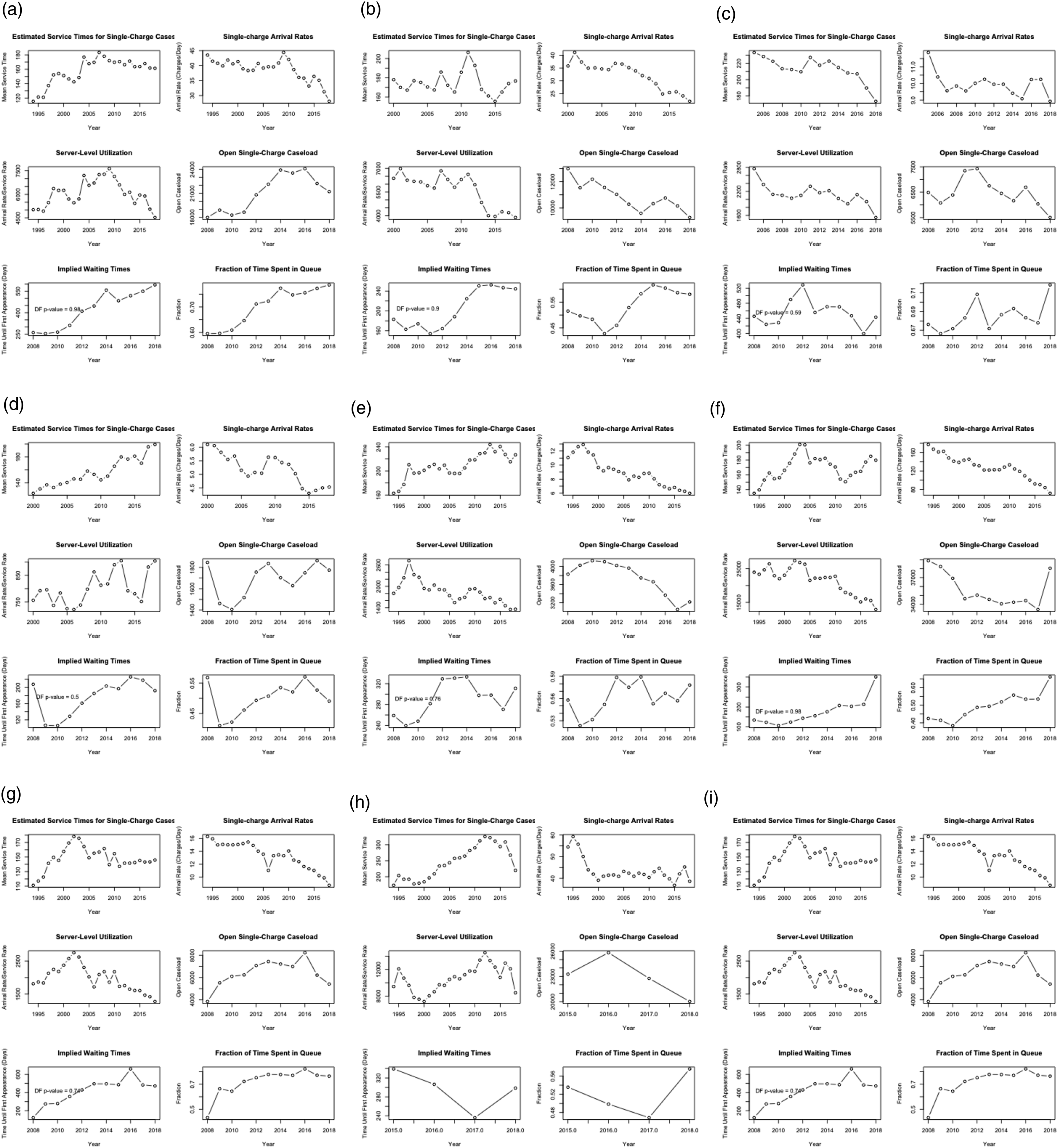

5. Remand

Up to and during trial, individuals not granted bail are held in remanded custody, sometimes referred to as pretrial custody. While a bail hearings are typically provided within three days, adjournments are possible if requested by either side or if administrative resources are inadequate. However, if bail is not granted, the accused is kept in custody leading up to trial, imposing an enormous limit on the liberty of the accused. The setting we examine is one where the population in pretrial custody is rapidly increasing across all jurisdictions. To what extent can our measures of the system explain the rise of the population in remand?

The central measure from queueing theory that we look to use is the utilization rate given that this is the measure we have the longest time series on. The server-level utilization rate is a key measure from queueing theory which all other measures, such as wait time and queue size, are increasing in. The key hypothesis from queueing theory is that the utilization rate will co-move positively with the population in pretrial custody if queueing theory can explain the secular rise in the population in pretrial custody. While we have a shorter time series on wait times and queue size, these might also co-move positively with the population in pretrial custody.

From a queueing perspective, the population in remand serves as a lower bound count of individuals in the system at any given point in time, with the caveat that some count of individuals in the system are not in remand, as they have been granted bail. Figure 15 plots the average count of individuals remanded in custody on the left axis and the utilization rate on the right axis over the 1994–2018 period. Movements in the system’s utilization rate are highly correlated with the average count remanded in custody. However, since the series are non-stationary, we must take care to ensure those correlations are not spurious. The Granger causality test is a statistical hypothesis test for determining whether one time series is useful in forecasting another.

Figure 15.

Average count in remand and utilization rate. Note. The figure plots the average count of the population in remanded custody on the right axis and the system’s utilization rate ρ_t = λ_t/μ_t on the left axis. (a) Alberta, (b) British Columbia, (c) Manitoba, (d) New Brunswick, (e) Nova Scotia, (f) Ontario, (g) Prince Edward Island, (h) Saskatchewan, (i) Quebec.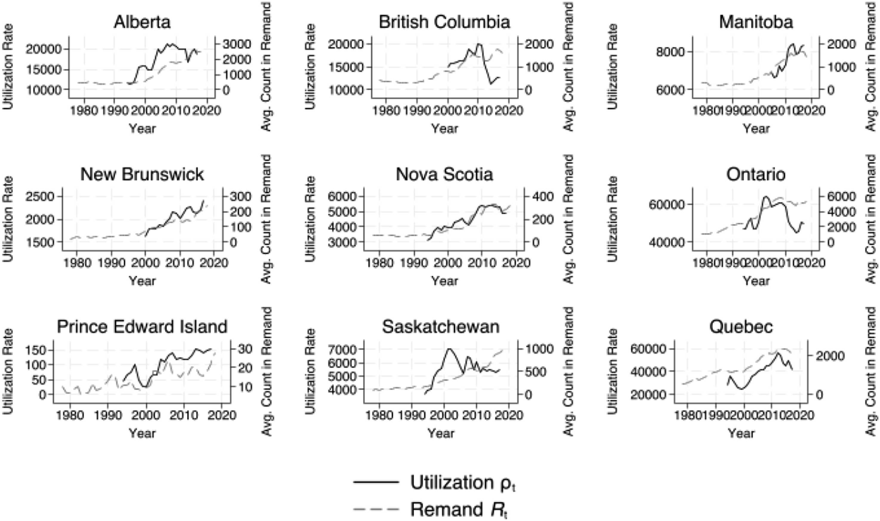

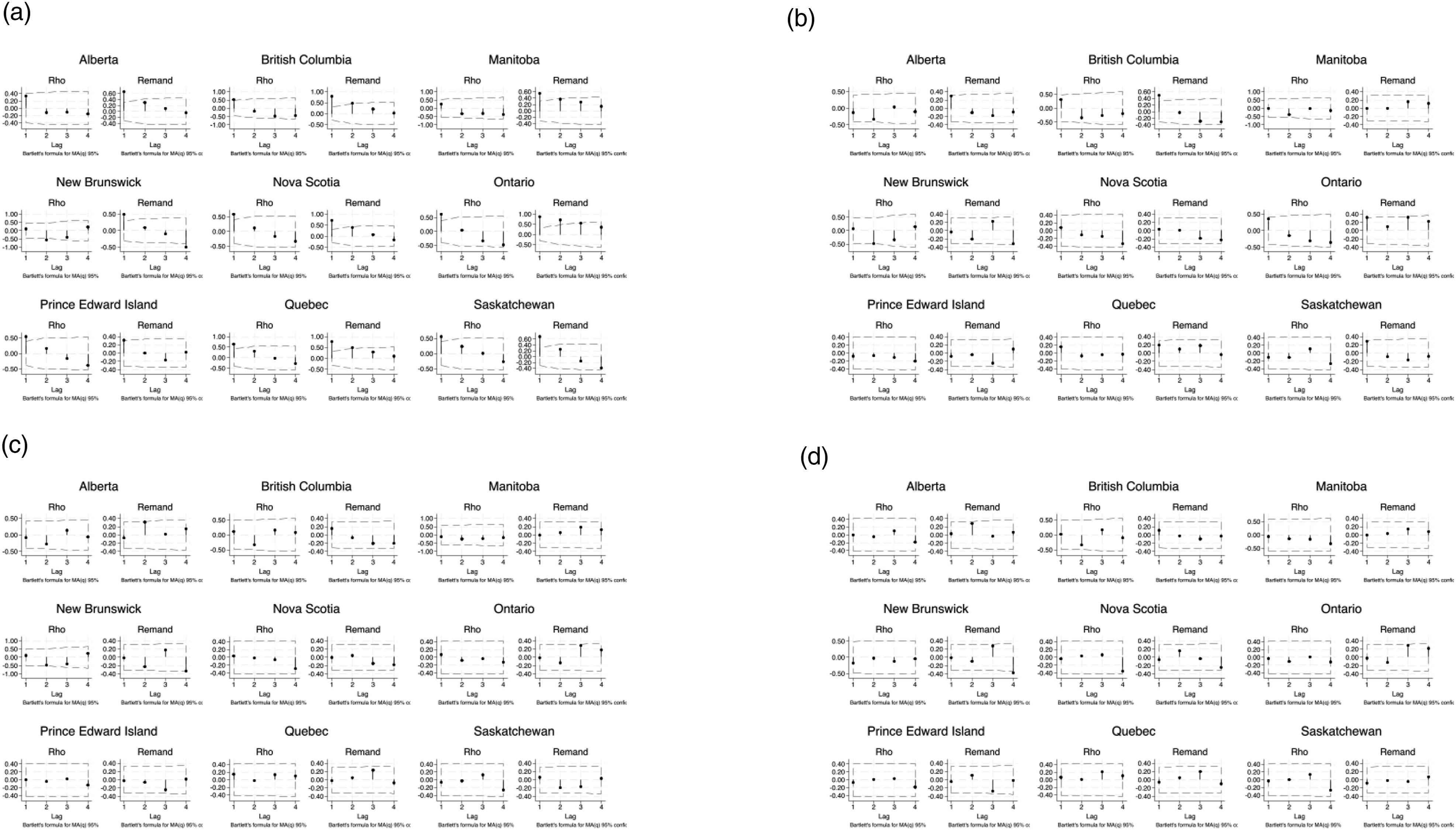
It can be seen immediately that both series are highly non-stationary, suggesting possible spurious correlation in their co-movement. In order to protect against the potential for spurious correlations, the series we compare must be stationary. Figure 16 plots series that have been adjusted in various ways to produce a stationary series. Figure 16(a) shows the remand and utilization series adjusted for a quadratic trend. Figure 16(b) shows the de-trended first differenced remand and utilization series. Figure 16(c) shows the remand and utilization residuals after adjusting for two independent AR(2) processes. Figure 16(d) shows the remand and utilization residuals from an AR(2) process after adjusting for a quadratic trend. Dickey-Fuller p values from a test for a unit root (non-stationarity) are shown. In general, all transformations produce stationary processes. Figure 17 plots the auto-correlation functions for four lags of each series by province. While the de-trended series appears to retain an AR(1) structure, the other adjustments, first differencing and AR(2) residuals, produce series that are approximately white noise.

Figure 16.

Remand and utilization adjusted time series. (a) Raw series adjusted for quadratic trend, (b) first difference series adjusted for linear trend, (c) residuals from AR(2) process, (d) residuals from AR(2) detrended process.

Figure 17.

Remand and utilization auto-correlation functions. (a) raw series adjusted for quadratic trend, (b) first difference series adjusted for linear trend, (c) residuals from AR(2) process, (d) residuals from AR(2) detrended process.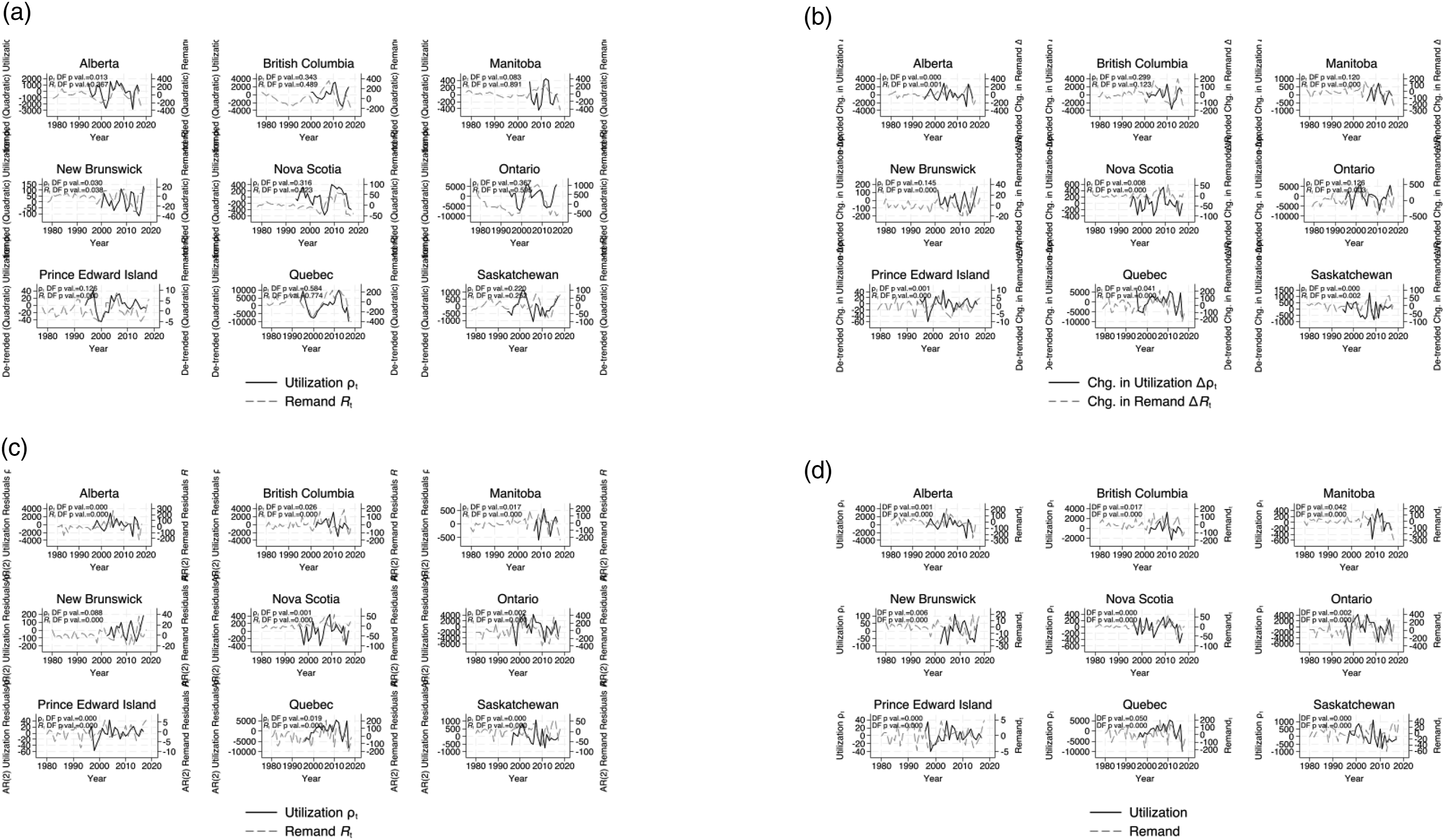

To detect co-movement between the utilization rate, the model’s measure of those being served, and the population remanded in custody, we run pooled time series regressions on adjusted series. Let R_pt denote the average population in remand and ρ_pt = λ_pt/μ_pt denote the utilization rate in province p in year t. Both utilization ρ_pt and remand R_pt are de-trended according to the following procedure. First, we estimate the following equation

Y_{p t} = α_{0} + α_{1} {YEAR}_{t} + γ_{2} {YEAR}_{t}^{2} + ϵ_{p t}

(13)

separately for each province and remand and utilization series Y_t ∈ {R_t, ρ_t}, where the YEAR and YEAR² variables account for a quadratic trend. Let

{\hat{ϵ}}^{Y}

denote the residuals of Y from the equation (13). Regressions using raw series are of the form

{\hat{ϵ}}_{p t}^{R} = β_{0} + β_{1} {\hat{ϵ}}_{p t}^{ρ} + η_{p t}

(14)

and first differenced regressions are of the form

Δ R_{p t} = γ_{0} + γ_{1} Δ ρ_{p t} + ε_{p t}

(15)

where Δ indicates the first difference between time t and t − 1. A time trend can be added easily to de-trend the first differenced series, just as with the raw series. Autoregressive AR(2) model residuals are obtained from regressions on the independent series according to

Y_{t} = δ_{0} + δ_{1} Y_{t - 1} + δ_{2} Y_{t - 2} + ζ_{t}

(16)

which is estimated separately for each province and remand and utilization series Y_t ∈ {R_t, ρ_t}. The residuals

\hat{ζ_{t}}

from the remand AR(2) procedure are then regressed on the residuals from the utilization AR(2) procedure in order to examine co-movement in the residual variation of the two series.

The results are presented in Table 5. All standard errors are CV3 jackknife standard errors clustered by province. After adjusting for a linear and quadratic trend and first differencing, the remand and utilization series co-move substantially with one another in virtually every specification. Only upon the inclusion of the transformed arrival rate does a statistically insignificant estimate on the utilization rate occur, but not when looking only at single-charge cases, our robustness check. The open caseload variable L_t shares no relationship with the population in remand, suggesting that queueing theory’s utilization measure can add predictive power relative to existing measures of the total number in the system. Indeed, we find a positive relationship between the de-trended wait time W_q and the average population in remand. The coefficient estimates from the first difference and AR(2) residual series imply a much smaller co-movement, but still a robust positive relationship. The AR(2) residuals for remand and utilization are plotted against one another in Figure 18.²⁰ Overall, the results suggest that there is statistically significant positive co-movement between the utilization and remand series.

Table 5.

Pooled Time Series Regressions.

	All Cases								Single-Charge Cases
	Levels					First Difference		AR(2) Residuals	Levels		First Difference		AR(2) Residuals
	(1)	(2)	(3)	(4)	(5)	(6)	(7)	(8)	(9)	(10)	(11)	(12)	(13)
Utilization ρ_pt	0.0311**	0.0306***	0.0197	0.0381***	0.0345***			0.0115***	0.0815***	0.0711***			0.0302***
Utilization ρ_pt	(0.0106)	(0.00835)	(0.0108)	(0.00878)	(0.00945)			(0.00284)	(0.00966)	(0.0175)			(0.00709)
Open Caseload L		0.0250
Open Caseload L		(0.0164)
Arrival Rate λ_t			8.062***							9.457
Arrival Rate λ_t			(0.965)							(7.117)
Queue Size L_q				0.0484**
Queue Size L_q				(0.0145)
Wait Time W_q					0.869*
Wait Time W_q					(0.466)
Chg. in utilization Δρ_pt						0.0177	0.0149*				0.0389**	0.0353***
Chg. in utilization Δρ_pt						(0.00998)	(0.00713)				(0.0141)	(0.00940)
Constant	0.258	1.143	0.0463	2.661	1.719	41.47**	3.819	10.75**	0.172	0.137	44.48**	4.029	10.82**
Constant	(6.271)	(5.831)	(6.330)	(5.658)	(5.859)	(12.54)	(3.209)	(4.062)	(6.303)	(6.314)	(14.07)	(3.229)	(4.098)
Observations	191	82	191	82	82	180	180	169	191	191	180	180	169
R-squared	0.113	0.099	0.152	0.119	0.095	0.094	0.072	0.043	0.067	0.082	0.047	0.041	0.033
Trend	Quadratic	Quadratic	Quadratic	Quadratic	Quadratic	None	Linear	None	Quadratic	Quadratic	None	Linear	None
HC3 Standard Error	0.0106	0.00835	0.0128	0.0272	0.0270	0.00690	0.00613	0.00515	0.0313	0.0361	0.0279	0.0246	0.0200
Clusters	9	9	9	9	9	9	9	9	9	9	9	9	9
Wild bootstrap p value	0.146	0.0610	0.198	0.0450	0.0710	0.0800	0.0850	0.176	0.0580	0.0740	0.0870	0.0970	0.234

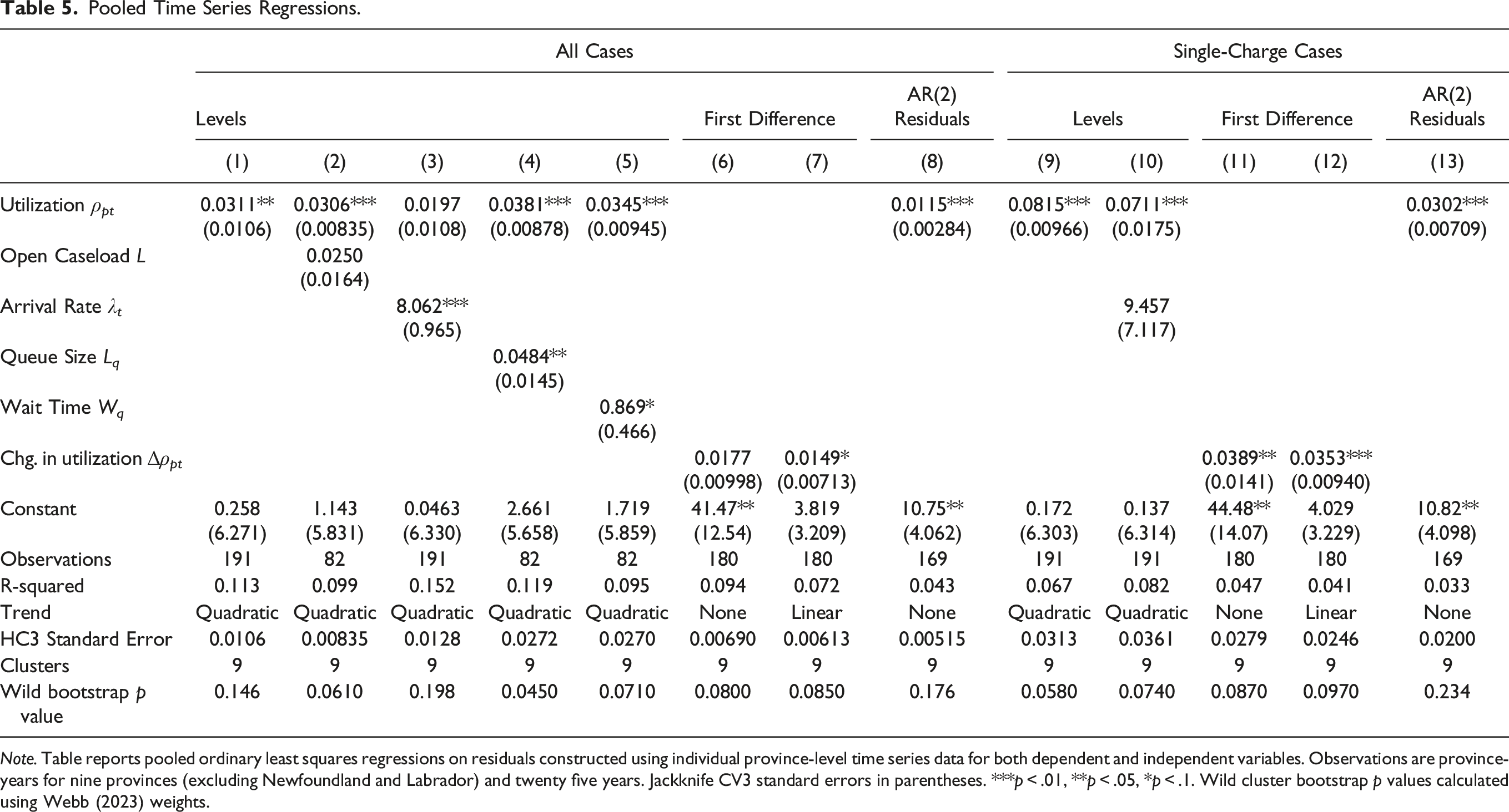
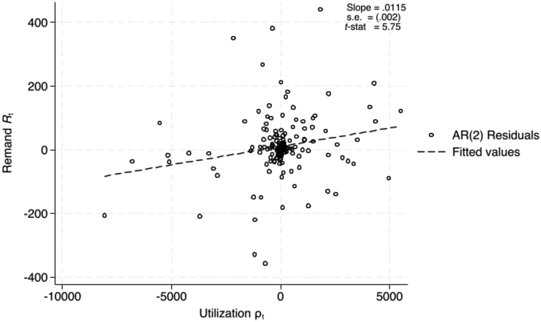
Note. Table reports pooled ordinary least squares regressions on residuals constructed using individual province-level time series data for both dependent and independent variables. Observations are province-years for nine provinces (excluding Newfoundland and Labrador) and twenty five years. Jackknife CV3 standard errors in parentheses. ***p $<$ .01, **p $<$ .05, *p $<$ .1. Wild cluster bootstrap p values calculated using Webb (2023) weights.

Figure 18.

Partial relationship between AR(2) remand and utilization residuals. Note. The figure plots AR(2) residuals from independent regressions according to equation (16) for remand and utilization series.

5.1. Robustness Check: Single-charge Cases

The court system manages many types of cases. One way of distinguishing between types of cases is by single- and multiple-charges. The queueing system can be “thinned” by simply analyzing the service time and arrival rate for single-charge cases only. This serves as a robustness check, as we are unable to observe the number of charges per information for multiple-charge cases, but also allows us to test the mechanisms which underly the relationship between our measure of congestion and the population in pretrial custody. Indeed, one might expect no relationship between measures of single-charge congestion and the population in pretrial custody, as these accused in these cases are much less likely to be detained in custody due to the fact that they face less serious charges.

Table 5 also displays the results testing for co-movement between the thinned single-charge queueing theory measures, such as utilization ρ_t and the arrival rate λ_t, and the total population in pretrial custody. Again, we detect strong co-movement between queueing theory’s measure of traffic congestion, the thinned utilization rate, and find that this measure outperforms conventional measures such as the thinned arrival rate. The inclusion of the arrival rate does not result in a statistically insignificant coefficient estimate on the utilization rate in single-charge cases. The coefficient estimate in column 12 of Table 5 implies that an increase of one hundred cases being served in the system per year leads to an increase of three in remanded custody. In general, the thinned utilization measure produces coefficient estimates that are larger than when analyzing the total system, both single- and multiple-charge cases. The increase in coefficient estimates suggests either that the results from the total utilization regressions suffered from measurement error which led to attenuation bias.

The results are remarkable in yet another way. That is, one would not expect that congestion of single-charge cases would be related to remand since they will be more likely to be granted low or no bail, as their charges are less serious. However, the robustness of the results bolster the conclusion that court congestion is the mechanism that is driving the troubling trends in the population in pretrial custody. Single-charge cases clog up the court system, leaving those in pretrial custody waiting longer for their date in court.

6. Conclusion

The right to be tried within a reasonable time is widely recognized as a pillar of criminal justice systems around the world. However, criticisms of the court system’s efficiency are abound. In 1971, William Landes noted in The Journal of Law and Economics that “[i]t is widely recognized that the courts are burdened with a larger volume of cases than they can efficiently handle” (p. 74). This is particularly important in the criminal procedure context where it has been argued that the long delays “blunt the deterrent effect of the criminal law” (Meador, 1972). The problem of court congestion is documented throughout history and remains just as relevant today as it was then, in particular in Canada, where the population in pretrial custody has exploded.

Our paper resolves the paradox of rising pretrial populations and falling crime rates by exploiting a basic framework from the field of operations research widely known as queueing theory. We use data on millions of criminal cases to estimate the service time distributions of provincial criminal justice systems over two decades. We find that the duration of criminal trials fit an exponential distribution well, suggesting that a memoryless queueing model might be appropriate. We then used queueing theory to construct a measure of court congestion, the utilization rate, which is a measure of the court’s traffic flow. In the infinite-server, memoryless model (i.e., M/M/∞), with no delay, this number reflects the total number in the system, an idealized measure of open caseload were there to be no delay or capacity in the system. We then use data on the court’s actual open caseload to back out measures of implied queue size and wait time until first appearance by exploiting a fundamental idea in queueing theory, which is that a system’s queue grows as utilization ρ and open caseload L diverge. Both measures, queue size and wait time, are, in general, increasing and non-stationary for the nine provinces we examine, suggesting that some criminal courts are at or near capacity and may be spiralling out of control. Overall, our data validates the widely-held impression that the court system, in particular, the criminal justice system, is over-burdened.

Using time series analysis, we also found positive co-movement between the model’s measures of congestion, the utilization rate, the queue size, and wait time, and the average count of the population in pretrial custody, suggesting that court congestion has explanatory power for the rise of the population in remanded custody. Measures from our multiple-server queueing model, such wait time and queue size, outperform the measures currently available to researchers in the raw data, such as open caseload, in predicting the population in pretrial custody. Building on the seminal contribution of McAllister et al. (1991), our research further validates the use of queueing theory for analyzing the criminal justice system.

These basic relationships validate the use of our measures for the study of other lines of inquiry. Future research may also wish to exploit the COVID-19 shock to examine the impact on court delay and its effect on other outcomes (see, e.g., Paciocco, 2021). Given the robustness of the relationship between the model’s measure of court congestion and the population in pretrial custody, future research may also wish to use our approach to estimating the delay of criminal trials to study other outcomes of interest in the criminal justice system, such as guilty pleas.

There are many policy conclusions to be gained from this exercise. First, we believe our measures of court performance constructed from publicly available data can be used going forward as a real-time performance measure of the court system that can be used in s. 11(b) constitutional litigation. Second, our results suggest that the duration and number of trials co-move positively with the population in pretrial custody. The measures recovered from our queueing model help resolve the paradox of falling crime with a rising population in pretrial custody.

Future research should attempt to use finer geographic data to focus in on where congestion is being generated. This may involve changing the unit of analysis from the province down to the courthouse. Future research may also take advantage of higher frequency data in order to obtain more precise estimates of the relationship between court congestion and remand, such as day-of-week and month effects, as well as seasonality. Because of the annual periodicity of our data, we are unable to validate that the arrival process is indeed Poisson. We simply take annual averages of cases. Higher frequency data would be required to know if the Poisson process is appropriate, such as, for instance, if inter-arrival times are exponentially distributed. We have documented how the maximum likelihood estimation procedure would need to be augmented in order to account for data on the number of charges per information.

One aspect of queueing theory that we are unable to speak to is the service discipline. We have combined multiple data sources and exploited Little’s Law to avoid specifying the underlying structure of the system, such as the service discipline or number of servers. In many places, our invocation of memorylessness was for the benefit of its utility. In reality, criminal court systems often employ service disciplines that look more like priority queueing or processor sharing than first-come first-serve. Future research should attempt to examine the effect of these service discplines have on the estimated delay of criminal trials. Rather, we have exploited Little’s Law, which does not depend on assumptions about the arrival process, the number of servers in the system, or the service discipline (Eilon, 1969; Jewell, 1967) and invoked memorylessness to study the behaviour of the model-implied queue.

A host of recent policies in Canada have been directed at reducing congestion in the criminal justice system: the hybridization of offences as either summary or indictable; the restriction on the use of the preliminary inquiry; and the framework set out by the nation’s highest court in Jordan. We leave future research to debate the relative merits of jury trials, preliminary hearings, and the court’s screening function against the costs of court congestion. While we leave these thorny normative questions about how best to perform legal triage for the subject of future research, we do arm researchers with reliable statistics from which they can develop designs that measure the effects of these policies on court congestion and case outcomes.

Supplemental Material

Supplemental Material - Estimating the Delay of Criminal Trials: Evidence From Canada

Supplemental Material for Estimating the Delay of Criminal Trials: Evidence From Canada by Dylan R. Clarke and Adam Metzler in Journal of Law & Empirical Analysis

Footnotes

Acknowledgments

We are grateful for very helpful comments from Steve Coughlan and Palma Paciocco, and Sam Kaufman and Diana Grech at the Ministry of the Attorney General for guidance on the data.

Declaration of Conflicting Interests

The author(s) declared no potential conflicts of interest with respect to the research, authorship, and/or publication of this article.

Funding

The author(s) received no financial support for the research, authorship, and/or publication of this article.

ORCID iD

Dylan R. Clarke

Supplemental Material

Supplemental material for this article is available online.

Notes

References

Canadian Charter of Rights and Freedoms, s 11, Part I of the Constitution Act, 1982, being Schedule B to the Canada Act 1982 (UK) . (1982). c11.

Criminal Code, RSC . (1985). c C-46.

Dobbie

Jacob

Yang

(2018). The effects of pretrial detention on conviction, future crime, and employment: Evidence from randomly assigned judges. The American Economic Review, 108(2), 201–240. https://doi.org/10.1257/aer.20161503

Eilon

(1969). A simpler proof of L = λW. Operations Research, 17(5), 915–917. https://doi.org/10.1287/opre.17.5.915

Gray v. Gray, 6 Ill. App. 2d 571 . (Ill. App. Ct. 1955). 128 N.E.2d 602.

Green

(2006). Queueing analysis in healthcare. In Hall

R. W.

(Ed.), Patient flow: Reducing delay in healthcare delivery. International series in operations research management science (Vol. 91, pp. 281–307). Springer. https://doi.org/10.1007/978-0-387-33636-710

Hlynka

(December 2017). History of queueing theory. Myron Hlynka’s Queueing Theory Page. https://web2.uwindsor.ca/math/hlynka/qhist.html (accessed May 1, 2021).

Jewell

W. S.

(1967). A simple proof of: L = λW. Operations Research, 15(6), 1109–1116. https://doi.org/10.1287/opre.15.6.1109

Kalven

Jr. (1963). General analysis of and introduction to the problem of court congestion and delay, A rules and procedures.1963 American Bar Association. Section of Insurance, Negligence and Compensation Law. Proceedings 322.

10.

Karam

Lukassen

Miladinovic

Wallace

(2020). Juristat. Statistics Canada Catalogue no. 85-002-X.

11.

Landes

W. M.

(1971). An economic analysis of the courts. The Journal of Law and Economics, 14(1), 61–104. https://doi.org/10.1086/466704

12.

Little

J. D.

(1961). A proof for the queuing formula: L = λW. Operations Research, 9(3), 383–387. https://doi.org/10.1287/opre.9.3.383

13.

McAllister

Atchinson

Jacobs

(1991). A simulation model of pretrial felony case processing: A queuing system analysis. Journal of Quantitative Criminology, 7(3), 291–314. https://doi.org/10.1007/bf01063235

14.

Meador

D. J.

(1972). Standards and goals for the courts. In Progress Report of the Nat’l Advisory Comm’n on Crim. Justice Standards and Goals, May, 1972, at 18 (4th Nat’l Symposium on Law Enforcement Science and Technology), 1–3 May, 1972.

15.

Mukherjee

Whalen

(2018). Priority queuing on the docket: Universality of judicial dispute resolution timing. Frontiers in Physics, 6. https://doi.org/10.3389/fphy.2018.00001

16.

Paciocco

(2021). Trial delay caused by discrete systemwide events: The post-Jordan era meets the age of COVID-19. Osgoode Hall Law Journal, 57(3), 835–867. https://doi.org/10.60082/2817-5069.3607

17.

Penney

Rondinelli

Stribopoulos

(2018). Criminal procedure in Canada (2nd ed.). Lexis Nexis.

18.

Petersen

(2020). Do detainees plead guilty faster? A survival analysis of pretrial detention and the timing of guilty pleas. Criminal Justice Policy Review, 31(7), 1015–1035. https://doi.org/10.1177/0887403419838020

19.

Ross

S. M.

(2010). Introduction to probability models: Academic Press.

20.

R v. Charley . (2019). ONCA 726.

21.

R v. Jordan . (2016). SCC 27.

22.

Statistics Canada . (2004). Victim participation in the plea negotiation process in Canada. https://www.justice.gc.ca/eng/rp-pr/cj-jp/victim/rr02_5/p0.html

23.

US Const amend VI .

24.

Webb

M. D.

(2023). Reworking wild bootstrap-based inference for clustered standard errors. Canadian Journal of Economics, 56(3), 839–858. https://doi.org/10.1111/caje.12661

25.

Yang

(2016). Resource constraints and the criminal justice system: Evidence from judicial vacancies. American Economic Journal: Economic Policy, 8(4), 289–332. https://doi.org/10.1257/pol.20150150

Supplementary Material

Please find the following supplemental material available below.

For Open Access articles published under a Creative Commons License, all supplemental material carries the same license as the article it is associated with.

For non-Open Access articles published, all supplemental material carries a non-exclusive license, and permission requests for re-use of supplemental material or any part of supplemental material shall be sent directly to the copyright owner as specified in the copyright notice associated with the article.

0.00 MB

0.31 MB