Sage Journals: Discover world-class research

Abstract

Chemometric regression models were developed for the quantification of praseodymium (Pr, 0–1000 µg/mL), neodymium (Nd, 0–1000 µg/mL), and nitric acid (HNO₃, 0.1–5 M) using spectrophotometry. Designed calibration sets were composed of 20 samples each: 10 model points and 10 lack-of-fit (LOF) points. The D-optimal designs effectively minimized the number of samples required to build models, and each design resulted in similar prediction performance, suggesting that statistical design of experiments can provide a reliable framework for selecting training set samples in three-variable systems. Partial least squares regression (PLSR) models were validated against a one-factor-at-a-time validation set composed of 125 samples (three variables, five levels). The top PLS-1 models resulted in average percent root mean square error of prediction error values of 3.5%, 1.7%, and 1.2% for Pr(III), Nd(III), and HNO₃, respectively. Power set augmentations of the model and LOF samples were investigated to optimize the number of training set samples. PLSR models built using just required model points (10) had similar predictive capabilities as models including the LOF points (20) but with fewer samples. The number of validation samples was also varied systematically to learn how many samples are needed to validate regression models. This work addresses long-standing questions in the field of chemometrics to help make this approach amenable to the near-real-time quantification of hazardous species in remote settings.

Graphical abstract

This is a visual representation of the abstract.

Keywords

Calibration approaches lanthanides optical spectroscopy machine learning online monitoring D-optimal design

Introduction

Optical spectroscopy and chemometric analysis can be applied for online monitoring of advanced chemical processing operations in numerous scientific fields. This method includes the analysis of materials in the nuclear field, where processing takes place in harsh environments (e.g., hot cells).^1–3 Traditional grab sample collection is cumbersome and expensive, but the analysis of process streams in situ, that is, within radiological environments, using fiber-optic cables provides a significant benefit. Online monitoring can help control product quality, improve process efficiency, maintain safety standards, and track material inventory.^3,4 Optical techniques provide not only the elemental composition of a process stream but can also provide chemical information pertaining to sample oxidation state(s), speciation, and chemical interactions.⁵

Various optical techniques and machine learning algorithms are available for such an analysis. One of the most traditional methods is known as spectrophotometry, or absorption spectroscopy, and provides a quantitative measure of sample absorption as a function of wavelength (nanometers). Traditionally, this approach is implemented for quantitative analysis using simple univariate regression methods, for example, Beer's law; however, recent advancements in chemometric analysis have enabled the analysis of complex samples with various matrices.^6–10

Model selection and the samples included in the training set, that is, calibration and validation samples, can be the trickiest and most crucial aspects of implementing machine learning techniques.^11–13 The bias–variance trade-off is important to consider with all supervised machine learning models, which estimate a relationship between X (spectra matrix) and the response matrix Y (concentration).^14–17 Calibration samples can determine how flexible a model is and how well it performs on unseen data.

A plethora of preprocessing and feature selection options are available to the researcher.¹⁸ Recent advancements in automation can make this process simpler for the user.^19,20 No universal approach exists for selecting calibration and validation samples to span the expected conditions.¹⁸ Training sets are often selected by the user and are subject to bias, and the number of samples needed can be ambiguous. Recent advancements in the application of experimental design for sample selection appear promising.^12,13 These samples are selected within a statistical framework and use metrics such as fraction of design space (FDS) to pinpoint the optimal number of samples.^21–24 The primary goal is generating a balanced sample distribution in any direction of the design space to ensure all points have reasonable influence on the solution, that is, partial least squares regression (PLSR) model.

Optimal designs are formed by solving for the solutions of various numerical criteria which are fundamentally different depending on the design type. The two most common criteria are the D-criterion (D-optimal) and I-criterion (I-optimal). The I-optimal variance is lower across the middle of the design space, and D-optimal designs perform better at the edges.²⁴ Thus, if the designed model needs to cover the entire concentration range, D-optimal designs may provide a more balanced estimate. Validation samples test a model's prediction performance on samples not included in the training set. The general rule of thumb is that the number of samples should be roughly the same as the samples in the calibration set. However, when working with designed sets that minimize the number of samples, this rule may not be the best approach.¹²

This work evaluated multiple PLSR models built from training sets selected by D-optimal design for the quantification of Pr (0–1000 parts per million, or ppm [µg/mL]), Nd (0–1000 ppm), and nitric acid (HNO₃, 0.1–5 M) using spectrophotometry. The prediction performance of each model was tested against a validation set composed of 125 samples, and power set augmentations were used to evaluate model performance as a function of samples included/excluded from the model and validation sets. Three points of scientific advancement are covered in this work: (i) PLSR models built using multiple D-optimal designs minimized the number of samples in the training sets with consistent prediction performance, (ii) the relationship between prediction performance uncertainty and the number of validation samples was determined, and (iii) a method to produce and validate predictive models with optimized training sets amenable to online monitoring applications in the nuclear field was developed. This work will support radioisotope production projects, such as the production of ¹⁴⁷Pm from neutron-irradiated Nd targets and other nuclear material processing scenarios involving actinides.^1,4,25,26

Experimental

Materials and Methods

Sample Preparation

Samples were prepared using volumetric pipettes and a balance with an accuracy of ±0.0001 g. Concentrations in the calibration and validation sets were chosen to span the range of anticipated conditions: Pr (0–1000 ppm), Nd (0–1000 ppm), and HNO₃ (0.1–5 M). Sample concentrations in the calibration set were selected using D-optimal designs. A one-factor-at-a-time (OFAT) approach was used to select validation set samples at the lowest level, and then 10%, 25%, 50%, and 100% of the highest level. Error propagation is outlined in Supplemental Material. Samples were prepared using deionized water with Millipore Sigma Milli-Q purity (18.2 MΩ cm at 25 °C).

Spectroscopic Measurements

Absorption spectra were collected using Ocean Insight QEPro (316–1105 nm) and NIRQuest (898–1705 nm) spectrophotometers. A 2 cm static quartz cuvette was used for each measurement, and the spectrophotometers were referenced to deionized water. A longer–path length cell (e.g., 5 cm) could be used to improve detection limits. Flow cells could readily be used in future experiments to enable in-line monitoring. Spectra were recorded in triplicate and processed using OceanView 2.0 software (Ocean Insight, USA). An incoherent light source (SL201L, Thorlabs) was transmitted through a 2 m fiber-optic cable (multimode, low-OH, 400 µm diameter, Thorlabs) to a variable–path length cuvette holder (Avantes). The light was collected using a bifurcated fiber bundle (Thorlabs) and sent to each spectrophotometer. All spectra were recorded at 20 °C at 0.5 s intervals. The spectrophotometers were referenced to pure Milli-Q water.

Design of Experiments

Design expert by StatEase was used to generate several D-optimal designs using a quadratic model (Tables S1–S3, Supplemental Material). These designs are computer-generated designs that satisfy the D-optimality criterion (i.e., minimizes the determinant of the Y′Y inverse concentration matrix). Each concentration level was treated as continuous levels and numeric factors. The 10 required model points were augmented with 10 lack-of-fit (LOF) points to improve the FDS. Six LOF points were required to achieve an FDS of 0.99. Four additional LOF points were included beyond the minimum number suggested by the design statistics using a delta (d) value of 2, a sigma (s) value of 1, and an alpha (α) of 0.05. The variable delta (d) describes the maximum acceptable half-width, that is, margin of error, sigma (s) is an estimate of the standard deviation, and alpha (α) is the significance level used in the statistical analysis. LOF points minimize the distance to other runs in the factor space and help improve the precision of the model. The validation set included the OFAT samples to test the prediction performance of each design. Three samples were left out of the OFAT set of 125 because of errors with sample preparation. OFAT levels of 0%, 10%, 25%, 50%, and 100% of the maximum expected concentrations were tested. The comparison of three D-optimal designs in this work could be extended to other optimal designs (e.g., I-optimal).

Multivariate Chemometrics

The SciKit Learn package in Python was used for building PLSR models. PLSR is one of the most common supervised regression methods that is useful for reducing the dimensionality of overdetermined spectral systems where the number of independent variables is much larger than the samples. This method models both X (spectra) and Y (concentration) matrices simultaneously to find the structure in X that best predicts that latent variables (LVs) in Y to maximize the covariance. A k-fold method, in which the calibration set is split into k random groups, then models are built iteratively using k – 1 groups to predict the kth group not included, was used for cross-validation. Model statistics are highly dependent on the validation method used and the number of LVs, that is, factors included in the model. Too many factors can overfit the model and include noise or other artifacts that inhibit model performance. For ease of comparing multiple models, the number of LVs was set to three. This amount is equal to the number of varying species in the study and the common inflection point in the prediction error versus LV curve for most models. Each model was built with a minimum baseline offset shift correction, which can help the model cope with fluctuations anticipated during process monitoring applications. Additional preprocessing strategies outlined in a previous work were also tested.⁸ These strategies include mean centering, standard normal variate (SNV), and Savitzky–Golay (SG) smoothing and derivative filters. SG filters are based on a local least squares fitting of the data by polynomials. Briefly, centering and scatter factors included two levels corresponding to no transformation or applying the transformation (two levels). The SG smoothing and derivative filters included combinations of zero-, first-, and second-order derivatives (three levels), with a first-, third-, fifth-, or seventh-polynomial order (four levels), and 2–30 left/right points (29 levels).

Statistics

The quality of the regression evaluated the root mean square error (RMSE) of the calibration (RMSEC), cross-validation (RMSECV), and prediction (RMSEP). RMSE is used to evaluate models because of its ability to evaluate the bias–variance trade-off. Models with high bias will consistently make incorrect predictions owing to a systematic error, whereas models with high variance may make correct predictions but will typically result in overfit models.¹⁷ The optimal model will balance these two variables. Cross-validation statistics can be somewhat inflated when designed calibration sets are used because each sample provides essential information; leaving one out has a negative effect on the calibration. This effect implies that RMSECV statistics may not accurately estimate model stability and the true prediction performance.²⁷ PLSR model prediction performance testing on samples not included in the training set is important because the RMSECV is only an estimate of the RMSEP, especially when using a designed sample matrix.⁵ RMSEs were calculated using Eq. 1,

RMSE = \sqrt{\frac{\sum_{i = 1}^{n} {({\hat{y}}_{i} - y_{i})}^{2}}{n}}

(1)

where

{\hat{y}}_{i}

is the predicted concentration, y_i is the measured concentration, and n is the number of samples. PLSR models were optimized by minimizing the RMSEP. Percent RMSEP was calculated by dividing the RMSEP by the median model values using Eq. 2,

\begin{matrix} RMSEP % = \frac{RMSEP}{y_{med}} \times 100 % \end{matrix}

(2)

where y_med represents the median of each analyte concentration range. RMSE values are in units of response variable y. Lower values indicate better model performance. Prediction performance is strong when percent RMSEP is less than 5%, satisfactory when percent RMSEP is less than or equal to 5 to 10%, and indicative when percent RMSEP is less than or equal to 10 to 15%.⁵ In addition to evaluating the RMSE values of PLSR models, the u versus t plots, which compare the model's x- and y-scores for each LV, were investigated to ensure linearity.

Results and Discussion

Absorption Spectra

Figure 1 shows the absorption spectrum of Nd(III) and Pr(III) in HNO₃ media from 400 to 1300 nm. The concentrations of Nd(III) and Pr(III) in these spectra were 1000 µg/mL, i.e., 1 ppm, and the HNO₃ concentration was varied from 0.1 to 5 M. The spectra contain numerous Pr(III) and Nd(III) absorption peaks corresponding to intra-4f transitions.^28,29 For Nd(III), each peak corresponds to transitions from the ground state (⁴I_9/2) to various excited states.³⁰ The effect of varying HNO₃ concentration on the individual absorption peaks is shown. With increasing HNO₃ concentration, each Nd(III) peak changes in either intensity or peak shape. The Nd(III) peak at 575 nm (⁴I_9/2 → ⁴G_5/2, ²G_7/2) is known to be hypersensitive to the local environment and shows appreciable sensitivity toward HNO₃. This sensitivity is likely because of coordination with nitrate anions (NO₃⁻).³¹ The hypersensitive 575 nm Nd(III) band redshifts from 574 to 580 nm, changes shape, and the absorbance increased. This result is consistent with pervious literature reports.^28,30 The covarying nature of this peak because of the dependence on Nd and HNO₃ concentrations is difficult to model using univariate methods. The absorption spectrum dependence on acid concentration is also prevalent in actinide systems containing Np, Pu, and other species.^1,4 Variations in the location and shape of Pr(III) peaks at 444, 470, 483, and 594 nm were less pronounced, but the peaks changed slightly mostly owing to peak broadening with increasing acid concentration.

Figure 1.

(a) Pr(III) and (b) Nd(III) absorption spectra from 420 to 1300 nm as the HNO₃ levels are varied. The inset plot in (b) shows the Nd(III) 579 nm peak shape change as acid levels are increased. Similar, although less severe, peak shifts and shape changes are seen in the other Pr(III) and Nd(III) absorption peaks. For reference, the Nd(III) peak near 580 nm redshifted with increasing HNO₃ and the NIR band near 1200 nm increased in magnitude with increasing HNO₃.

Additionally, broad near-infrared (NIR) water absorption bands with negative absorbance values were identified with maximum values near 960 and 1200 nm. These bands correspond to overtones and fundamental OH^- vibrations of water, as previously described.^10,32,33 The ions H⁺ and NO₃^– do not absorb NIR radiation directly but instead distort the local tetrahedral structure of water. NIR absorption bands are also sensitive to temperature and ionic strength. Concentrations of Pr(III) and Nd(III) were too low in this study to affect NIR water band features. The spectrum was truncated at 1300 nm because of the high absorbance of the first overtone of water, which saturated the detector around 1440 nm. These nonlinear, covarying, and overlapping spectral characteristics were modeled with PLSR to build predictive models for quantification, and the spectra corresponding to various analyte concentrations were chosen by design of experiments.

Training Sets

The performance of predictive regression models such as PLSR depends significantly on the number and type of samples in the training set, and the number of samples directly affects the end user with respect to resources such as time and waste. The training set contains both calibration and validation samples. Minimizing samples in the training set can help make the chemometric approach more amenable to applications in restrictive environments, where fewer samples can help streamline operations and where material for calibration is limited. Beyond that minimization, a designed approach may help ensure consistent and representative sample sets for chemometric applications in all fields.

No universally accepted methods exist for selecting these samples, but sample selection often relies on the tacit knowledge of the user. Testing each point within the design space is challenging and nearly impossible. It is up to the researcher to decide whether the location of OFAT samples, D-optimal samples, or some other set in the design space is sufficient to train a model. A 3D plot of the entire three-variable design space is shown in Figure 2. An OFAT approach is commonly used in the literature; however, this approach results in numerous samples when each analyte is varied at five levels (5³= 125 samples), is impractical for applications above three analytes, for example, 5⁴= 625 samples, is often subject to user bias, and can result in overfitting, in which a model captures noise in addition to underlying patterns in the data. To address these issues, optimal design of experiments, for example, D-optimal designs, were chosen to minimize the samples in the training set, mitigate user bias in sample selection, and provide a consistent statistical framework by which samples can be selected within a given design space. However, underfitting can happen if too few samples are included in the calibration, which results in a model that has high bias and low variance and does not capture the underlying patterns in the data.

Figure 2.

The position of the OFAT and an example D-optimal sample plans within the three-variable design space.

Another challenge similarly important to the calibration set is ensuring that the number of validation samples used to validate the calibrated model properly evaluates the true predictive performance. A small subset of samples may represent the variation in the dataset, but the subset could also result in local minima and maxima and could suggest that a supervised model has better or worse performance than it actually does. The number of samples could also be system-dependent. In simple additive systems in which interionic associations and other chemical equilibria are negligible, it is conceivable that very few samples are necessary to build robust models. On the other hand, a larger number of samples may be required in more complex systems with broad signatures, peak shifts, multicollinearity, overlapping spectral features, and other effects that could result in singularities. Thus, developing a standardized sample selection method based on robust statistics and corroboration with experimental data is essential.

The D-optimal design did not include each vertex point but may describe enough variation to define score/loading relationships and regression coefficients that accurately account for the entire space (Figure 2). This design likely holds true in simpler systems in which interionic associations and other chemical equilibria are negligible. Previous work has compared the prediction performance of different statistical designs, but the authors are unaware of studies that have compared replicates of supposedly equivalent designs. These designs must be evaluated to determine how well the approach can be extended to other systems and replicated by researchers from one location to the next. These iterative, computer-driven designs are statistically equivalent per FDS criteria; however, each iteration does not generate the exact same samples each time.^20,21 Although the design statistics may be equivalent, the resulting prediction performance of chemometric regression models may not be. Each D-optimal design generated in this work contained 20 samples: 10 required model points plus another 10 LOF points (Tables S1–S3, Supplemental Material). An FDS of 0.99 was achieved with 16 samples in the model, but several additional samples were included in the design to determine if additional samples improved prediction performance. If additional LOF points improved the performance, it would imply that a higher-order model, for example, cubic, could be needed to generate a representative design. The concentration matrices and resulting spectra from each design and the OFAT method were evaluated to determine the number of calibration samples and the number of validation samples. These data lead to the primary question: How much of a given design space must be evaluated to account for spectral features related to all conceivable combinations of sample concentrations?

Full-Spectrum PLSR Models

The PLS-1 models for each D-optimal design were built using the entire spectrum from 400 to 1080 nm. These models were built from data that were only modified with a simple baseline offset correction. PLS-1 models were built for HNO₃ using both the region from 400 to 1080 nm collected with the QEPro spectrometer and the NIR region from 900 to 1300 nm with the NIRQuest spectrometer. Three LVs were used to describe the structured variation in the dataset for each model and each analyte to keep this variation consistent. This consistency is reasonable considering three analytes were being modeled. The number of LVs was confirmed by the last significant decrease in RMSE (Figure S1, Supplemental Material).

The RMSEP and percent RMSEP values for each PLS-1 model are shown in Table S4 (Supplemental Material). Slight differences were observed for the Pr models developed from each D-optimal design (RMSEP% = 8.4%–11.2%), but the Nd predictions were nearly identical (RMSEP% ≈ 3.2%) for each design. The PLS-1 models for HNO₃ using the NIRQuest data region significantly outperformed (RMSEP% = 2.0%–3.7%) the PLS-1 models built using QEPro data (9.2%–11.7%). Without trimming, both Nd and HNO₃ models achieved strong predictive capabilities by reaching the desired performance of percent RMSEP < 5%; however, Pr missed this mark. Therefore, the spectral region included in the regression analysis was trimmed to exclude variables with noise or little value for the regression.

It is common practice to remove deleterious artifacts to improve the correlation of X and Y data matrices. Here, the spectra were trimmed to only include areas where absorbance peaks for the corresponding analyte were present. The regression coefficients for non-trimmed models with three LVs are shown in Figure S2 (Supplemental Material). Although regression coefficients alone are not a perfect identifier of vital features, in this case, they aligned with known absorbance features serving as a logic check for the trimming selections. For example, the HNO₃ model generated from the QEPro data included the NIR water band near 960 nm and the Nd(III) peak near 581 nm. This Nd peak corresponds to the hypersensitive Nd(III) peak and the portion of the peak that grows with increasing HNO₃ concentration. A second round of PLS-1 models were evaluated after trimming.

PLSR Model Comparison

The PLS-1 model RMSEP statistics lowered slightly when only regions corresponding to absorbance features of interest were included in the model. Trimming the models lowered the average percent RMSEP for Pr and Nd by 17% and 15%, respectively, but increased the QEPro and NIRQuest acid models 24% and 4.7%, respectively (Table I). An alternative version of the table providing figures of merit for bias and variance is provided in Table S5 (Supplemental Material). In addition to feature selection, preprocessing transformations can improve the regression.

Table I.

Results for trimmed PLSR models.

	Preprocessing	LVs	RMSEP (ppm)	RMSEP% (%)	Wavelength filter (nm)
Pr
D-(A)	–	3	32.7	6.6	430–500 and 565–615
D-(B)	–	3	49.2	9.8	–
D-(C)	–	3	44.5	8.9	–
D-(A)-P	(0, 2, 3, 53, 0)	3	20.1	4.0	–
D-(B)-P	(0, 1, 3, 57, 0)	3	17.5	3.5	–
D-(C)-P	(0, 1, 3, 61, 0)	3	17.4	3.5	–
Nd
D-(A)	–	3	14	2.7	500–600 and 700–900
D-(B)	–	3	13	2.5	–
D-(C)	–	3	15	2.9	–
D-(A)-P	(0, 1, 7, 33, 0)	3	8.3	1.7	–
D-(B)-P	(0, 1, 7, 29, 0)	3	9.5	1.9	–
D-(C)-P	(0, 2, 3, 41, 0)	3	14	2.8	–
QEPro HNO₃
D-(A)	–	3	0.17	14	900–1080
D-(B)	–	3	0.15	12	–
D-(C)	–	3	0.15	12	–
D-(A)-P	(0, 1, 3, 17, 0)	3	0.14	12	–
D-(B)-P	(0, 0, 7, 41, 0)	3	0.13	11	–
D-(C)-P	(0, 0, 1, 61, 1)	3	0.14	11	–
NIRQuest HNO₃
D-(A)	/	3	0.052	2.1	900–1300
D-(B)	/	3	0.029	1.2	–
D-(C)	/	3	0.032	1.3	–
D-(A)-P	(0,1,3,61,0)	3	0.043	1.7	–
D-(B)-P	(0,0,7,9,0)	3	0.029	1.2	–
D-(C)-P	(0,0,7,9,0)	3	0.033	1.3	–

*A, B, C, D, and E correspond to SNV, derivative order, polynomial order, window size, mean centering (MC) under preprocessing. The wavelength filter for each section is the same as what is listed in the section's first row.

Transformations can be applied to spectral data to remove or minimize effects that do not contain beneficial information for the regression and to improve the interpretability of the data and models. Preprocessing significantly lowered the average percent RMSEP for the Pr models from 8.4% to 3.7% and only lowered RMSEP slightly for the other models (Table I). The application of preprocessing reduced the average model bias by 77% and 29% for Pr and Nd, respectively (Table S5). Similarly, preprocessing reduced the standard error of prediction, a measure of variance, by 47% and 20% for Pr and Nd, respectively. The QEPro HNO₃ preprocessed models saw a notable reduction in bias (53%) but an increase in variance, and the NIRQuest HNO₃ preprocessed models only saw minimal reductions in both bias and variance. Preprocessing lowered percent RMSEP for Pr, Nd, QEPro HNO₃, and NIRQuest HNO₃ by 56%, 23%, 11%, and 7%, respectively. Trimming and preprocessing lowered Pr prediction performance to achieve less than the target 5% threshold.

A total of 576 preprocessing combinations area described in a previous work⁸ and were evaluated using a Python script. The scatter correction (SNV) and mean centering were not selected for any of the models. On the other hand, SG derivative and smoothing filters were selected for each model. Mean centering refers to subtracting the average spectrum from each spectrum in the dataset. Identical filters for the models generated from each design were not chosen, but overall, SG window sizes and polynomial orders were consistent. The standard deviation of percent RMSEP values between each D-optimal model for Pr, Nd, QEPro HNO₃, and NIRQuest HNO₃ were 0.30%, 0.58%, 0.52%, and 0.58%, respectively. The percent relative standard deviations (RSDs) of percent RMSEP varied from 5% to 27%, which suggests that each design resulted in similar prediction performance. A slight difference in RMSEP between each design may not be related to statistical differences in the design itself but could be related to any number of user-related sources of variation (e.g., cuvette placement, sample preparation). A detailed evaluation of human error in this system could be pursued in future work.

In each case, beside the QEPro HNO₃ model, the designed approach resulted in PLSR models with strong prediction performance. A parity plot for each analyte is shown in Figure 3, comparing each D-optimal model's predictions to the 1 : 1 line (excluding the QEPro HNO₃ model results). Even though these models were built using just 20 samples, the prediction of the much-larger OFAT sample set was excellent.

Figure 3.

Parity plots comparing known to three preprocessed D-optimal calibrated model predicted values for Pr(III), Nd(III), and HNO₃. The 1 : 1 line represents a perfect prediction.

Attempts were also made to model Pr, Nd, and HNO₃ using only the region from 560 to 610 nm, which encompassed overlapping Pr and Nd peaks and the hypersensitive Nd(III) peak. This extremely trimmed model did not perform as well, particularly for HNO₃ concentration (data not shown here). Because the QEPro HNO₃ model did not achieve the target level of prediction performance (RMSEP% < 5%), it was left out of subsequent analyses in the following sections.

OFAT Model Predicting D-Optimal Sets

To cross-validate model performance as a function of samples in the calibration and validation sets, PLS-1 models were built using the OFAT samples (calibration) to predict each set of 20 D-optimal samples (validation). Spectral regions were trimmed in the same way as the D-optimal models. The no-preprocessing and preprocessing model RMSEP and percent RMSEP values are shown in Table II. The resulting average percent RMSEP for Pr, Nd, and HNO₃ were 4.6%, 3.4%, and 1.7%, respectively. Despite fewer samples in the validation set, the percent RMSEP values for Pr and Nd were 0.98% and 1.3%, respectively, higher on average than the D-optimal models predicting the OFAT samples. This result was contrary to the average percent RMSEP for the OFAT model predicting HNO₃ concentration in the D-optimal samples, which lowered by 1.1%.

Table II.

OFAT model RMSEP and percent RMSEP statistics.

	Preprocessing	LVs	RMSEP (ppm)	RMSEP% (%)
Pr
OFAT D-(A)	–	3	45	8.9
OFAT D-(B)	–	3	61	12.1
OFAT D-(C)	–	3	50	10.0
OFAT D-(A)-P	(0, 1, 3, 49, 0)	3	23	4.7
OFAT D-(B)-P	(0, 1, 3, 49, 0)	3	27	5.4
OFAT D-(C)-P	(0, 1, 3, 49, 0)	3	19	3.9
Nd
OFAT D-(A)	–	3	15	2.9
OFAT D-(B)	–	3	30	6.1
OFAT D-(C)	–	3	18	3.5
OFAT D-(A)-P	(0, 2, 7, 33, 0)	3	10	2.0
OFAT D-(B)-P	(0, 2, 7, 57, 0)	3	25	4.9
OFAT D-(C)-P	(0, 0, 1, 61, 0)	3	16	3.1
NIRQuest HNO₃
OFAT D-(A)	–	3	0.051	2.1
OFAT D-(B)	–	3	0.035	1.4
OFAT D-(C)	–	3	0.040	1.6
OFAT D-(A)-P	(0, 0, 7, 9, 0)	3	0.055	2.2
OFAT D-(B)-P	(0, 0, 7, 9, 0)	3	0.036	1.4
OFAT D-(C)-P	(0, 0, 3, 61, 0)	3	0.038	1.5

*A, B, C, D, and E correspond to SNV, derivative order, polynomial order, window size, and mean centering (MC) under preprocessing.

The RMSEC and RMSECV (k = 5) for the OFAT PLS-1 models and average RMSEP of the D-optimal trained models are shown in Table III. The RMSEC and RMSECV are similar, which indicates that the model is balanced. Interestingly, the RMSECV and average RMSEP of the D-optimal models are very similar, which suggest that each D-optimal model effectively captures the variation in the OFAT set. This suggests that approximately 20 samples for the D-optimal sets are sufficient to capture the prediction variation. However, additional tests were needed to determine if 20 samples were ideal or if even that set contained some redundancy.

Table III.

OFAT RMSEC and RMSECV compared with average RMSEP values from the D-optimal models without preprocessing.

Analyte	RMSEC	RMSECV (k = 5)	RMSEP D-optimal
Pr	31.0	40.9	42.2
Nd	8.3	15.6	13.6
NIRQuest HNO₃	0.024	0.067	0.038

Calibration Power Sets

Additional PLS-1 models were built using varying numbers of calibration samples through power set augmentation. Here, power set augmentation refers to the generation of all possible combinations of samples included in the overall sample set with groups ranging in size from one to the size of the overall sample population. For example, if the calibration set included (a,b,c), the power sets would be (a), (b), (c), (a,b), (a,c), (b,c), (a,b,c). These power set augmentations of the calibration set were analyzed in two groups: (i) Models were built with varying combinations of the 10 required model points, and (ii) models were built with the model samples plus varying combinations of the 10 LOF points. The average RMSEP values for each combination of 3–10 required model point combinations and each D-optimal design are shown in Figure 4. As the number of model points included in the calibration set increased, the RMSEP decreased, as expected. The RMSEP values for Pr, Nd, and HNO₃ for models built using all 10 required model points were 24 ppm, 11 ppm, and 0.078 M, respectively (RMSEP% = 4.8%, 2.2%, and 3.2%, respectively). These values were very similar to the models generated from all 20 D-optimal samples (see Table II). This result implies that the LOF points included in the model may not have provided substantial benefits to the performance.

Figure 4.

RMSEP versus the number of samples in the calibration set for (a) Pr and Nd and (b) HNO₃. Error bars represent one standard deviation.

Several combinations of five or six samples slightly outperformed the entire set of 10 samples (Figure S3); however, the difference in RMSEP is likely insignificant. The savings regarding material use and researcher time to prepare and analyze this smaller set of samples is significant (50%–60% reduction). The set with one of the lowest RMSEPs for Pr contained six samples out of the set of 10 required model points (Table S6, Supplemental Material). The RMSEP for this set was 25% lower than the RMSEP for the entire set of 10 samples. This minimized set contained four vertex points, one plane point, and one edge point in the design. These six points included both zero Pr and the highest concentration of Pr at both the lowest and highest HNO₃ concentrations. Thus, it is reasonable to think that PLSR could define scores, loadings, and regression coefficients with this small number of samples to cover the design space because no singularities or chemical equilibria occurred over the studies’ range to alter the spectral response at different concentration levels. Even if five or six samples do not provide a realistic, immediate benefit because at least 10 samples need to be analyzed to determine which ones are best empirically, the benefit would occur when deploying these models and rebuilding calibration models over time in a more restrictive production setting.

Although several combinations of four to six required model point samples outperformed the entire set of 10 samples, these were singularities in some because many other points were above the final RMSEP. Thus, selecting these samples a priori could not be achieved using a D-optimal design with a quadratic process order model. The three independent sets of 10 required model points performed much more consistently.

The second exercise was completed with the model samples plus varying combinations of the 10 LOF points. This exercise revealed that including additional LOF points in the model did not significantly improve prediction performance, that is, lower RMSEP. The RMSEP values for Pr, Nd, and HNO₃ were 18 ppm, 11 ppm, and 0.066 M, respectively. Including two times the number of samples lowered RMSEP by 24%, 8.0%, and 15%, respectively, when 20 samples were included in the calibration set, but each set was below the target of RMSEP% < 5% prior to the inclusion of these LOF samples. The percent reduction in RMSEP relative to the number of samples in the set suggests that if time and resources were constrained in any way, then just 10 samples would be ideal.

Validation Power Sets

One rule of thumb in the field of chemometrics is that the number of validation samples should balance the number of samples in the calibration set. However, when working with a designed sample set with minimal samples, this rule may or may not apply. This work assumed that the OFAT set of samples capture all possible spectral variations in the data and represents the entire design space. To evaluate the prediction performance of each D-optimal design (20 samples) with a varying number of validation samples, 100 random combinations of the OFAT samples were used to validate each model, with the number of validation samples used being varied from 1 to 120.

The average Pr model RMSEP for each sample combination as a function of the number of samples is shown in Figure 5. The same behavior was seen for all models and each analyte (data not shown here). After five samples, the average matched the true mean for the entire OFAT set. However, the percent RSD was rather large, which indicated that there was a large spread of RMSEP values when only five samples were used. This variability means that using just five samples resulted in both good RMSEP values and poor RMSEP values, but in either case, the true mean was not identified. It was not until combinations of 40 samples were evaluated that the percent RSD reached a reasonable level of 10%.

Figure 5.

(a) D-optimal designs’ RMSEP values for Pr shown as a function of the number of samples in the validation set, and (b) the average percent RSD as a function of the number of samples in the validation set.

Because of the random combinations used in lieu of the computationally expensive true power set (>10⁶ combinations), it is possible that the spread around the mean is inflated owing to imbalanced validation sets being tested across the design space. Because the LOF points were shown to provide little benefit for enhanced prediction power, it was hypothesized that these 10 samples could be used as a validation set because they inherently cover most of the design space. Additionally, with only 10 samples to consider, power set augmentations of the validation set were feasible (1023 combinations).

In this work, PLSR models were built with only the 10 required model samples, then evaluated for every possible combination of the 10 LOF samples as the validation set. These combinations ranged from 1 to 10 samples, with the spread of the RMSEP decreasing as the number of validation samples increased. Figure 5b shows that with 10 validation samples, the average percent RSD around the mean is approximately 20%. If this value is taken as the uncertainty of these LOF validation set RMSEPs, then there is good agreement with the OFAT validation RMSEPs–apart from D-optimal (2) for Nd. These values are compared for each system in Table IV.

Table IV.

Comparison of OFAT validation sets and the LOF validation sets.^a

	RMSEP% (%)
	Pr		Nd		NIRQuest HNO₃
	OFAT	LOF	OFAT	LOF	OFAT	LOF
D-optimal (1)	4.7	5.9 ± 1.2	1.6	1.9 ± 0.4	3.9	2.9 ± 0.6
D-optimal (2)	5.3	5.9 ± 1.2	2.6	9.5 ± 1.9	3.4	4.5 ± 0.9
D-optimal (3)	4.3	3.1 ± 0.6	2.5	2.4 ± 0.5	2.0	2.4 ± 0.5

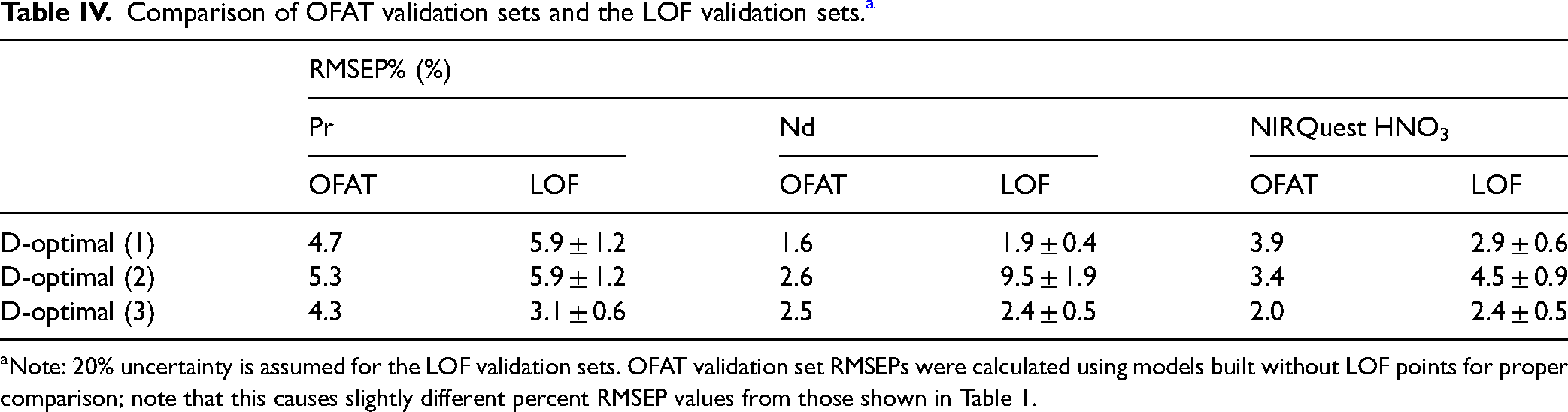
Note: 20% uncertainty is assumed for the LOF validation sets. OFAT validation set RMSEPs were calculated using models built without LOF points for proper comparison; note that this causes slightly different percent RMSEP values from those shown in Table 1.

When investigating the RMSEP versus number of validation samples plots for these LOF power sets, an added benefit was found. In many cases, a band of poorly predicted combinations would appear on the plot of RMSEP versus validation set size. Upon further investigation it was found that this band of poor predictions was the result of samples being included in the validation set combination (see Figure S4, Supplemental Material). This issue revealed cases in which certain LOF points were indeed needed in the model, and thus, these LOF samples could be moved to the calibration set for the final models. Investigation of this power set plot for the D-optimal (2) Nd model revealed that several (6 out of 10) LOF samples predicted poorly, which resulted in the inflated percent RMSEP value shown in Table IV. In this case, additional samples would need to be made to validate the model after these LOF points were moved into the calibration set. These samples did not reduce the prediction performance for Nd of the D-optimal (2) design when the required model points were also included (Table II). Overall, this power set evaluation of the LOF points as a validation set serves as an adequate measure of the true predictive accuracy of the model and a way to selectively improve the models by incorporating LOF points when truly needed.

Conclusion

Spectrophotometry and chemometric modeling performed well in characterizing Pr (0–1000 ppm), Nd (0–1000 ppm), and HNO₃ (0.1–5 M) concentrations. This good performance was due in part to a preprocessing approach and feature selection through PLSR model coefficients. Low prediction uncertainties, measured as the percent RMSEP, suggested that this approach could be successful in monitoring process streams. The minimized training set selected by D-optimal design was validated against a much larger OFAT set to show that fewer than 10 samples were sufficient to train predictive models to describe the design space. However, when the number of samples in the calibration set resulted in an FDS less than 0.99, the variation in prediction performance increased relative to the sample set size. Additionally, a validation strategy using a power set evaluation of D-optimal design LOF points effectively estimated the true RMSEP of the models while simultaneously identifying important LOF points. This result, along with comparable performance between PLSR models built using statistically equivalent D-optimal designs, suggests that designed approach for selecting training set samples is robust, flexible, and amenable to spectroscopy and chemometric studies within and beyond the nuclear field.

Supplemental Material

sj-docx-1-app-10.1177_27551857241243083 - Supplemental material for Comparing Designed Training Sets to Optimize Multivariate Regression Models for Pr, Nd, and Nitric Acid Using Spectrophotometry

Supplemental material, sj-docx-1-app-10.1177_27551857241243083 for Comparing Designed Training Sets to Optimize Multivariate Regression Models for Pr, Nd, and Nitric Acid Using Spectrophotometry by Luke R. Sadergaski, Hunter B. Andrews, David Rai II and Vasileios A. Anagnostopoulos in Applied Spectroscopy Practica

Footnotes

Acknowledgments

The authors wish to thank the US Department of Energy Isotope Program Core R&D for funding.

Author Contributions

The manuscript was written using contributions of all authors. All authors have given approval to the final version of the manuscript.

Declaration of Conflicting Interests

The authors declared no potential conflicts of interest with respect to the research, authorship, and/or publication of this article.

Funding

The authors disclosed receipt of the following financial support for the research, authorship, and/or publication of this article: Funding for this work was provided by US Department of Energy Isotope Program.

ORCID iDs

Luke R. Sadergaski

Hunter B. Andrews

Supplemental Material

All supplemental material mentioned in the text is available in the online version of the journal.

Notes

References

Lascola

O’Rourke

P.E.

Kyser

E.A.

. “A Piecewise Local Partial Least Squares (PLS) Method for the Quantitative Analysis of Plutonium Nitrate Solutions”. Appl. Spectrosc. 2017. 7(12): 2579–2594. https://doi.org/10.1177/0003702817734000

Sadergaski

L.R.

Depaoli

D.W.

Myhre

K.G.

. “Monitoring the Caustic Dissolution of Aluminum Alloy in a Radiochemical Hot Cell Using Raman Spectroscopy”. Appl. Spectrosc. 2020. 74(10): 1252–1262. https://doi.org/10.1177/0003702820933616

Kirsanov

Rudnitskaya

Legin

Babain

. “UV–Vis Spectroscopy with Chemometric Data Treatment: An Option for On-Line Control in Nuclear Industry”. J. Radioanal. Nucl. Chem. 2017. 312: 461–470. https://doi.org/10.1007/S10967-017-5252-8

Sadergaski

L.R.

Myhre

K.G.

Delmau

L.H.

. “Multivariate Chemometric Methods and Vis-NIR Spectrophotometry for Monitoring Plutonium-238 Anion Exchange Column Effluent in a Radiochemical Hot Cell”. Talanta Open. 2022. 5: 100120. https://doi.org/10.1016/J.Talo.2022.100120

H.B. Andrews, L.R. Sadergaski. “Leveraging Visible and Near-Infrared Spectroelectrochemistry to Calibrate a Robust Model for Vanadium(IV/V) in Varying Nitric Acid and Temperature Levels”. Talanta. 2023. 259: 124554. https://doi.org/10.1016/J.Talanta.2023.124554

Tse

Shafer

Bryan

S.A.

Nelson

G.L.

Lines

A.M.

. “Measuring Nd(III) Solution Concentration in the Prescence of Interfering Er(III) and Cu(II) Ions: A Partial Least Squares Analysis of Ultraviolet–Visible Spectra”. Appl. Spectrosc. 2022. 76(2): 173–183. https://doi.org/10.1177/00037028211053852

Lackey

H.E.

Sell

R.L.

Nelson

G.L.

Bryan

T.A.

Lines

A.M.

Bryan

S.A.

. “Practical Guide to Chemometric Analysis of Optical Spectroscopic Data”. J. Chem. Educ. 2023. 100(7): 2608–2626. https://doi.org/10.1021/Acs.Jchemed.2c01112

L.R. Sadergaski, T.J. Hager, H.B. Andrews. “Design of Experiments, Chemometrics, and Raman Spectroscopy for the Quantification of Hydroxylammonium, Nitrate, and Nitric Acid”. ACS Omega. 2022. 7(8): 7287–7296. https://doi.org/10.1021/acsomega.1c07111

Casella

A.J.

Levitskaia

T.G.

Peterson

J.M.

Bryan

S.A.

. “Water O–H Stretching Raman Signature for Strong Acid Monitoring via Multivariate Analysis”. Anal. Chem. 2013. 85(8): 4120–4128. https://doi.org/10.1021/Ac4001628

10.

L.R. Sadergaski, S.B. Irvine, H.B. Andrews. “Partial Least Squares, Experimental Design, and Near-Infrared Spectrophotometry for the Remote Quantification of Nitric Acid Concentration and Temperature”. Molecules. 2023. 28(7): 3224. https://doi.org/10.3390/Molecules28073224

11.

C. Beleites, R. Salzer. “Assessing and Improving the Stability of Chemometric Models in Small Sample Size Situations”. Anal. Bioanal. Chem. 2008. 390(5): 1261–1271. https://doi.org/10.1007/S00216-007-1818-6

12.

Sadergaski

L.R.

Toney

G.K.

Delmau

L.H.

Myhre

K.G.

. “Chemometrics and Experimental Design for the Quantification of Nitrate Salts in Nitric Acid: Near-Infrared Spectroscopy Absorption Analysis”. Appl. Spectrosc. 2021. 75(9): 1155–1167. https://doi.org/10.1177/0003702820987281

13.

R.W. Bondi Jr, J.K.B. Igne,C.A. Drennen III. “Effect of Experimental Design on the Prediction Performance of Calibration Models Based on Near-Infrared Spectroscopy for Pharmaceutical Applications”. Appl. Spectrosc. 2012. 66(12): 1442–1453. https://doi.org/10.1366/12-06689

14.

Mehta

Bukov

Wang

C.-H.

Day

A.G.R.

, et al. “A High-Bias, Low-Variance Introduction to Machine Learning for Physicists”. Phys. Rep. 2019. 810: 1–124. https://doi.org/10.1016/j.physrep.2019.03.001

15.

J. Rocks, P. Mehta. “Memorizing Without Overfitting: Bias, Variance, and Interpolation in Overparameterized Models”. Phys. Rev. Res. 2022. 4: 013201. https://doi.org/10.1103/physrevresearch.4.013201

16.

Chan

J.Y.-L.

Leow

S.M.H.

Bea

K.T.

Cheng

W.K.

, et al. “Mitigating the Multicollinearity Problem and Its Machine Learning Approach. A Review”. Mathematics. 2022. 10(8): 1283. https://doi.org/10.3390/Math10081283

17.

N.K.M. Faber. “A Closer Look at the Bias-Variance Trade-Off in Multivariate Calibration”. J. Chemom. 1999. 13(2): 185–192. https://doi.org/10.1002/(SICI)1099-128X(199903/04)13:2<185::AID-CEM538>3.0.CO;2-N

18.

Engel

Gerretzen

Szymanska

Jansen

J.J.

, et al. “Breaking with Trends in Pre-Processing?”. Trends Anal. Chem. 2013. 50: 96–106. https://doi.org/10.1016/j.trac.2013.04.015

19.

Kappatou

C.D.

Odgers

García-Muñoz

Misener

. “An Optimization Approach Coupling Preprocessing With Model Regression for Enhanced Chemometrics”. Ind. Eng. Chem. Res. 2023. 62(15): 6196–6213. https://doi.org/10.1021/Acs.Iecr.2c04583

20.

H.B. Andrews, L.R. Sadergaski, S.K. Cary. “Pursuit of the Ultimate Regression Model for Samarium(III), Europium(III), and LiCl Using Laser-Induced Fluorescence, Design of Experiments, and a Genetic Algorithm for Feature Selection”. ACS Omega. 2023. 8(2): 2281–2290. https://doi.org/10.1021/Acsomega.2c06610

21.

Johnson

R.T.

Montgomery

D.C.

Jones

B.A.

. “An Expository Paper on Optimal Design”. Qual. Eng. 2011. 23(3): 287–301. https://doi.org/10.1080/08982112.2011.576203

22.

Zahran

Anderson-Cook

C.M.

Myers

R.H.

. “Fraction of Design Space to Assess Prediction Capability of Response Surface Designs”. J. Qual. Technol. 2003. 35(4): 377–386. https://doi.org/10.1080/00224065.2003.11980235

23.

Wold

Josefson

Gottfries

Linusson

. “The Utility of Multivariate Design in PLS Modeling”. J. Chemom. 2004. 18(3–4): 156–165. https://doi.org/10.1002/Cem.861

24.

B. Smucker, M. Krzywinski, N. Altman. “Optimal Experimental Design”. Nat. Methods. 2018. 15(8): 559–560. https://doi.org/10.1038/S41592-018-0083-2

25.

Sadergaski

L.R.

Andrews

H.B.

Wilson

Queern

S.L.

Hunley

R.D.

. “Feasibility Study of Spectrophotometry to Support a Promethium Production Program at ORNL”. In: ORNL/TM-2022/2505. Oak Ridge, TN: Oak Ridge National Laboratory, 2022. https://info.ornl.gov/sites/publications/Files/Pub179169.pdf [accessed Mar 14 2024]. 10.2172/1885315.

26.

Upson

U.L.

Wheelwright

E.J.

. In-Cell Recording Optical Spectrometer”. BNWL-337. Richmond, WA: Battelle Northwest Laboratory, 1967). https://www.osti.gov/servlets/purl/4441388 [accessed Mar 14 2024]. 10.2172/4441388).

27.

Cederkvist

H.R.

Aastveit

A.H.

Naes

. “A Comparison of Methods for Testing Differences in Predictive Ability”. J. Chemom. 2005. 19(9): 500–509. https://doi.org/10.1002/Cem.956

28.

Picayo

G.A.

Etz

B.D.

Vyas

Jensen

M.P.

. “Characterization of the ALSEP Process at Equilibrium: Speciation and Stoichiometry of the Extracted Complex”. ACS Omega. 2020. 5(14): 8076–8089. https://doi.org/10.1021/acsomega.0c00209

29.

Carnall

W.T.

Fields

P.R.

Rajnak

. “Electronic Energy Levels in the Trivalent Lanthanide Aquo Ions. I. Pr³⁺, Nd³⁺, Pm³⁺, Sm³⁺, Dy³⁺, Ho³⁺, Er³⁺, and Tm³⁺”. J. Chem. Phys. 1968. 49(10): 4424–4442. https://doi.org/10.1063/1.1669893

30.

Kumar

Maji

Sundararajan

. “Nd(III) Hypersensitive Peak as an Optical Absorption Probe for Determining Nitric Acid in Aqueous Solution: An Application to Aqueous Raffinate Solutions in Nuclear Reprocessing”. Talanta. 2021. 231: 122398. https://doi.org/10.1016/J.Talanta.2021.122398

31.

L. Rao, G. Tian. “Complexation of Lanthanides with Nitrate at Variable Temperatures Thermodynamics and Coordination Modes”. Inorg. Chem. 2009. 48(3): 964–970. https://doi.org/10.1021/ic801604f

32.

Beganovic

Moll

Huck

C.W.

. “Comparison of Multivariate Regression Models Based on Water- and Carbohydrate-Related Spectral Regions in the Near-Infrared for Aqueous Solutions of Glucose”. Molecules. 2019. 24(20): 3696. https://doi.org/10.3390/Molecules24203696

33.

Chang

Shinzawa

Chung

. “Concentration Determination of Inorganic Acids that Do Not Absorb Near-Infrared (NIR) Radiation Through Recognizing Perturbed NIR Water Bands by Them and Investigation of Accuracy Dependency on Their Acidities”. Microchem. J. 2018. 139: 443–449. https://doi.org/10.1016/j.microc.2018.03.019

Supplementary Material

Please find the following supplemental material available below.

For Open Access articles published under a Creative Commons License, all supplemental material carries the same license as the article it is associated with.

For non-Open Access articles published, all supplemental material carries a non-exclusive license, and permission requests for re-use of supplemental material or any part of supplemental material shall be sent directly to the copyright owner as specified in the copyright notice associated with the article.

0.00 MB

2.06 MB

Comparing Designed Training Sets to Optimize Multivariate Regression Models for Pr,Nd,and Nitric Acid Using Spectrophotometry

Abstract

Keywords

Introduction

Experimental

Materials and Methods

Sample Preparation

Spectroscopic Measurements

Design of Experiments

Multivariate Chemometrics

Statistics

Results and Discussion

Absorption Spectra

Training Sets

Full-Spectrum PLSR Models

PLSR Model Comparison

OFAT Model Predicting D-Optimal Sets

Calibration Power Sets

Validation Power Sets

Conclusion

Supplemental Material

sj-docx-1-app-10.1177_27551857241243083 - Supplemental material for Comparing Designed Training Sets to Optimize Multivariate Regression Models for Pr, Nd, and Nitric Acid Using Spectrophotometry

Footnotes

Acknowledgments

Author Contributions

Declaration of Conflicting Interests

Funding

ORCID iDs

Supplemental Material

Notes

References

Supplementary Material