
Abstract
Cash is an important strategic asset for firms and scholars have a longstanding interest in the optimum level of a firm's cash holdings. In this study, we revisit the relationship between cash holdings and firm value by conducting a re-examination of Kim and Bettis, who hypothesized and found positive but decreasing marginal returns of cash. We argue and demonstrate that the regression model configuration of Kim and Bettis leads to distorted regression results. Once we adjust their regression model configuration, our results show that the benefits of cash do not diminish but instead increase with increasing cash holdings. In further analyses, we find indicative evidence that these results may be driven by firms with very high investment opportunities. We also employ a larger sample over a longer period of time to corroborate the time generalizability of our findings, we perform several checks to establish their robustness, and we discuss their theoretical implications.
Introduction
Cash has become a major asset for firms (Bates, Kahle, & Stulz, 2009). In fact, firms’ cash-to-assets ratios have grown substantially over recent decades. Bates et al. (2009) reported that the average cash ratio in their sample increased from about 10% in 1980 to about 23% in 2006. This means that the average firm in 2006 could retire all of its debt obligations with its cash holdings (Bates et al., 2009: 1985). Headed by large technology companies like Apple, Alphabet, and Microsoft, S&P 500 companies in early 2022 had enough cash to give more than $8,000 to every person in the United States (Krantz, 2022). In fact, Apple alone reported having more than $200 billion in cash and investments. To put this number into perspective it is helpful to recall that this is almost the GDP of Greece (World Bank, 2023). This “massive cash pile” that such companies are “sitting on” has also been on the minds of investors who frequently call for dividends and stock buybacks (Krantz, 2022).
Given this prominence of cash, and strategy scholars’ fundamental interest in firm performance, it is not surprising that there has long been an interest in the relationship between cash holdings and firm value (e.g., Mikkelson & Partch, 2003). The cash–performance relationship is especially intriguing as the optimum level of a firm's cash holdings represents a theoretical conundrum (George, 2005). On the one hand, agency theory highlights the costs of large cash holdings such as giving rein to managers’ self-serving tendencies (Jensen, 1986). Large cash holdings reduce resource constraints and agency theory posits that large cash holdings therefore give managers the discretion to use corporate resources ineffectively (see George, 2005). In case of large cash holdings, managers are no longer forced to be resourceful, for example, not taking burdensome actions of bootstrapping, which causes allocative efficiency to deteriorate. On the other hand, the behavioral theory of the firm highlights the benefits of large cash holdings for resolving latent intra-organizational conflicts (Cyert & March, 1963). For instance, large cash holdings may allow opposing parties inside a firm to coexist harmoniously by pursuing their own ideas and projects (see George, 2005). Large cash holdings relax internal controls and thereby also create funds that allow for an environment of innovation, in which projects with uncertain outcomes are acceptable.
Consequently, scholars have empirically examined the effect of cash on firm performance (e.g., Oler & Picconi, 2014) and interactions with factors such as governance (e.g., Pinkowitz, Stulz, & Williamson, 2006), accounting practices (e.g., Louis, Sun, & Urcan, 2012), or competition (e.g., Fresard, 2010). Depending on such factors, cash holdings can be positively related, unrelated, or negatively related to firm value (e.g., Frésard & Salva, 2010; Kalcheva & Lins, 2007).
Notably, Kim and Bettis (2014) conducted a particularly influential study on the subject. They theorized and concluded from their empirical analysis that (a) the cash–performance relationship “takes the form of a quadratic function with a positive original term and a negative squared term,” that is, an inverted U-shape, and that (b) the “interaction of cash holdings with firm size is positively related to firm value” (Kim & Bettis, 2014: 2056, 2057). Their research has been impactful (e.g., Deb, David, & O’Brien, 2017; Vanacker, Collewaert, & Zahra, 2017) and practically and theoretically important as their results call for large cash holdings, challenging the predictions of agency theory.
However, beyond the fact that every study that was worth doing in the first place is worth to be re-examined (Bettis, Ethiraj, Gambardella, Helfat, & Mitchell, 2016a; Bettis, Helfat, & Shaver, 2016b), there are several reasons that warrant a re-examination of this seminal study. First, the study's sampling frame ranges from 1988 to 2009, so one may question the generalizability of the results to the present day, especially against the backdrop of today's firms holding larger amounts of cash than ever. Second, and more importantly, we propose that the regression model configuration which Kim and Bettis (2014) used to test their two hypotheses can lead to distorted results. Due to their chosen measurement of the dependent variable (i.e., Tobin's q), the independent variable's numerator (i.e., cash and short-term investments) is part of the dependent variable's numerator (i.e., market value of the firm) and denominator (i.e., total assets). A change in the independent variable's numerator can therefore unintendedly affect the dependent variable, which makes their regression model configuration prone to spurious effects. Finally, Kim and Bettis (2014) did not differentiate between firms with different investment opportunities in their testing of the cash–performance relationship. This potentially obscures useful insights because the benefits of cash may materialize differently depending on the investment opportunities available to a firm. After all, only if a firm possesses valuable investment opportunities in the first place can cash enable the firm to seize opportunities and implement value-creating projects swiftly. Hence, only a high level of investment opportunities may allow adaptive benefits of cash to fully unfold. In sum, these concerns prevent us from being unreservedly confident in the findings on the cash–performance relationship by Kim and Bettis (2014).
In this article, we therefore examine the robustness and generalizability of the results of Kim and Bettis (2014) with respect to the hypothesized relationships between cash holdings, size, and firm value. We do so in four steps. Following recommended re-examination procedures (Ethiraj, Gambardella, & Helfat, 2016), we start with a literal (i.e., narrow) reproduction (Köhler & Cortina, 2023). We then alter Kim and Bettis’ (2014) measurement of the dependent variable (i.e., Tobin's q) to allow for undistorted regression results. Next, we check our inferences by examining how generalizable they are across time (Zhao & Murrell, 2016). We employ a sample that includes the observations of Kim and Bettis (2014) and extends their time frame. Compared to Kim and Bettis (2014), our sample size is up to 38% larger, adding over 24,000 firm-year observations. Thereupon, we perform a sample split (Aouadi & Marsat, 2018; see Hansen, 2000) to separately examine the cash–performance relationship for firms with low investment opportunities, firms with moderately high investment opportunities, and firms with very high investment opportunities. After this four-step re-examination, we provide further robustness checks.
Like O’Brien and Folta (2009) as well as Kim and Bettis (2014), we find a positive cash–performance relationship. But in contrast to Kim and Bettis (2014), we observe increasing marginal returns when analyzing our entire sample. In more fine-grained analyses, our results provide initial evidence that the cash–performance relationship Kim and Bettis (2014) reported (i.e., an inverted U-shape with a turning point at a high cash level) may only hold for firms with moderately high investment opportunities. For firms with low investment opportunities, we find an inverted U-shape with a turning point at a low cash level. For firms with very high investment opportunities, however, we find a U-shaped (i.e., positive squared term) relationship between cash holdings and firm value. Instead of decreasing marginal returns of cash, as hypothesized and reported by Kim and Bettis (2014), we thus find increasing marginal returns of cash for these kinds of opportunity-rich firms. Finally, our results provide support for Kim and Bettis’ (2014) hypothesized positive cash–size interaction effect.
We contribute to the discussion on the theoretically important and practically relevant relationship between cash holdings and firm value by refining methodology and offering additional empirical evidence (Ethiraj et al., 2016). Our results suggest that large cash holdings create costs, as put forth by agency theory (Jensen, 1986), and yield benefits, as proposed by the behavioral theory of the firm (Cyert & March, 1963). Importantly, such benefits may materialize differently for firms depending on the investment opportunities available to them. Cash holdings beyond the level that a firm needs to meet its transaction needs hardly yield any benefits for firms with low investment opportunities. Hence, the costs of large cash holdings tend to dominate for such firms. Firms with low investment opportunities might do best if they focus on their deployed assets, distribute excess cash to shareholders, and develop new investment opportunities. The higher the investment opportunities available to a firm, the more the benefits of large cash holdings unfold. In these cases, investors appear to value the buffer and option qualities of large cash holdings, and thus their favorable effect on firms’ abilities to fully reap current and future investment opportunities. This occurs to an extent such that the benefits of large cash holdings tend to dominate for firms with high investment opportunities. Our research, therefore, helps to clarify the interplay between the opposite effects proposed by agency theory and the behavioral theory of the firm regarding the optimal level of a firm's cash holdings.
Theoretical background
The appropriate level of a firm's cash holdings is subject to a theoretical trade-off. Specifically, agency theory (e.g., Jensen, 1986) and the behavioral theory of the firm (e.g., Cyert & March, 1963) assess the costs and benefits of holding cash differently. While classical economic and behavioral approaches are not mutually exclusive (Levinthal, 2011), these two theory streams reach different conclusions when it comes to determining the appropriate level of a firm's cash holdings. Drawing on Kim and Bettis (2014: 2054–2055), we outline their stances on the appropriate level of a firm's cash holdings in the following.
From an agency theory point of view, it is appropriate to hold just enough cash to meet transaction needs. The only benefit of holding cash is seen as facilitating required cash payments in a smooth way. Holding more cash than necessary to meet transaction needs is seen as financially wasteful as cash on a firm's bank account yields relatively low returns and incurs substantial opportunity costs because it is not being deployed to financially lucrative investments either inside or outside the firm. Excess cash is seen as a symptom of managerial inefficiency and/or self-serving behavior, which reduces shareholder wealth (Jensen, 1986). Thus, large cash holdings are seen as poor corporate governance. If excess cash exists, it should be either invested in value-creating projects, that is, projects that have “positive net present values when discounted at the relevant cost of capital” (Jensen, 1986: 323), inside the firm or paid to shareholders by means of dividends and/or share repurchases such that it can be invested in value-creating projects outside the firm.
From a behavioral theory of the firm point of view, it can be appropriate to hold more cash than is necessary to meet transaction needs because cash is a type of slack. Such slack allows firms to adapt (see Cyert & March, 1963) because it helps firms to resolve internal conflicts and to hedge external uncertainty by means of side-payments, that is, payments compensating specific negative effects. Cash can function as a buffer in these cases. For example, firms pursuing a strategy of innovation typically face higher uncertainty causing a greater need for internal buffers and such firms will therefore benefit especially from financial slack (O’Brien, 2003). Similarly, the buffering quality of cash can foster creativity and even fortuitous discoveries and inventions because it reduces constraints and allows for experimentation. Large cash holdings can also buffer against economic downturns and provide the flexibility to make long-term investments. Finally, excess cash helps to overcome the tendencies of risk-averse managers who allocate too little resources to uncertain but valuable projects. Cash as a buffer in case of failure motivates risk-taking (Jeffrey, Onay, & Larrick, 2010) and thereby prevents managers’ risk-aversion from hurting firm performance because it counteracts the negative effects of managerial risk-aversion on firm innovation.
Combining these two points of view, we see that there exist two countervailing forces that jointly shape the cash–performance relationship. While agency theory highlights the costs of large cash holdings such as giving rein to managers’ self-serving tendencies (Jensen, 1986), the behavioral theory of the firm highlights the benefits of large cash holdings such as resolving latent intra-organizational conflicts (Cyert & March, 1963).
Building on these two theoretical perspectives, Kim and Bettis (2014: 2055) argued for (a) linearly increasing opportunity costs of cash once a firm's cash holdings go beyond the cash level necessary to meet transactional needs and (b) asymptotically increasing adaptive benefits of cash. As a result, Kim and Bettis (2014: 2056) derived their first hypothesis:
Hypothesis 1: “The relationship between cash holdings and firm value takes the form of a quadratic function with a positive original term and a negative squared term.”
In addition to theorizing this inverse U-shaped relationship, Kim and Bettis (2014: 2056–2057) further hypothesized that firm size moderates the effect of cash holdings on firm performance. Building on the concept of scale economies of cash based on the premise that large firms have certain competitive advantages over small firms regarding competitive deterrence (e.g., Caves & Porter, 1977), Kim and Bettis (2014) argued that firm size will positively moderate the cash–performance relationship. The key idea is that, if a large and a small firm both hold the identical proportion of their assets in cash, the larger firm will have higher absolute cash holdings than the smaller firm. Assuming that (a) strategic deterrence is one of the benefits of holding cash and that (b) strategic deterrence is amplified by an incumbent's absolute investment power, such higher absolute cash holdings then allow the larger firm to more effectively deter known and unknown (potential) competitors by increasing their uncertainty of success and lowering their expected returns. Larger absolute cash holdings would then indeed present a more credible threat to competitors. In other words, competitive deterrence is seen as exhibiting absolute scale economies (e.g., launching future advertising campaigns). As a result, Kim and Bettis (2014: 2057) derived their second and final hypothesis:
Hypothesis 2: “The interaction of cash holdings with firm size is positively related to firm value.”
Four-step re-examination
In this section, we examine the robustness and generalizability of the results of Kim and Bettis (2014) with respect to the hypothesized relationships between cash holdings, size, and firm value. Our re-examination comprises four steps. We start with a literal reproduction. We then alter Kim and Bettis’ (2014) measurement of the dependent variable (i.e., Tobin's q). Next, we check our inferences by examining how generalizable they are across time. Thereupon, we perform a sample split to separately examine the cash–performance relationship for firms with low, moderately high, and very high investment opportunities. We describe the methods and results of each step in the following.
Literal reproduction (step 1)
Following recommended re-examination procedures (Bettis et al., 2016b; Ethiraj et al., 2016), we start with a literal, also called narrow or direct, reproduction (Köhler & Cortina, 2023). This reproduction matches the empirical setting and research design of Kim and Bettis (2014) as closely as possible, to calibrate our procedure with their original study.
Methods
Following the original study, we use the CRSP-COMPUSTAT merged database to build the first sample, which includes firm-year observations from 1988 to 2009 (Kim & Bettis, 2014: 2057). We measure all variables following Kim and Bettis (2014: 2058, 2059). Regarding the dependent variable, Tobin's q is measured as the market value of the firm—that is, “the sum of calendar-year end values of the firm's common stock (PRCC_C × CSHO), market value of the firm's preferred stock (PSTK), book value of the firm's long-term debt (DLTT), and book value of the firm's short-term debt with a maturity less than 1 (DD1)”—divided by total assets (AT) (Kim & Bettis, 2014: 2058). Regarding the explanatory variables, cash stock is measured as cash holdings, that is, cash and short-term investments (CHE), divided by total assets (AT), and firm size is measured as the natural logarithm of the number of total employees (in thousands) (Kim & Bettis, 2014: 2058, 2059). Regarding the measurement of the additional control variables, we follow Kim and Bettis (2014: 2059) and “take year fixed effects to account for unobservable macroeconomics effects [and] control for industry fixed effects by using three-digit SIC codes.” In terms of statistical methods, we follow the original study, which detects first-order autocorrelation in the data, and hence use the Prais and Winsten (1954) approach with robust standard errors. In terms of statistical software, we use Stata 15.1.
Results
When we first estimated the regression models with the specifications described above, we, like Kim and Bettis (2014), found support for hypothesis 1. For hypothesis 2, however, we obtained an interaction effect between cash and size that was materially different from the result they reported. We suspected that outliers in the sample caused the deviation in the result because the specifications that Kim and Bettis (2014) used in their main regression models did not fully control for the (potential) confounding effects of outliers (see their Footnote 4). Therefore, we winsorized the dependent variable, that is, Tobin's q, and the two explanatory variables, that is, cash and size, at the bottom 1% and top 1% level (e.g., Flammer & Kacperczyk, 2019; Shan, Fu, & Zheng, 2017). Table 1 provides the descriptive statistics and the correlation matrix for the variables in our re-examination samples. 1 Panel A of Table 1 reports the sample using the time period of Kim and Bettis (2014). Panel B of Table 1 reports the sample using our longer time period which is later used in step 3.
Descriptive statistics and correlations
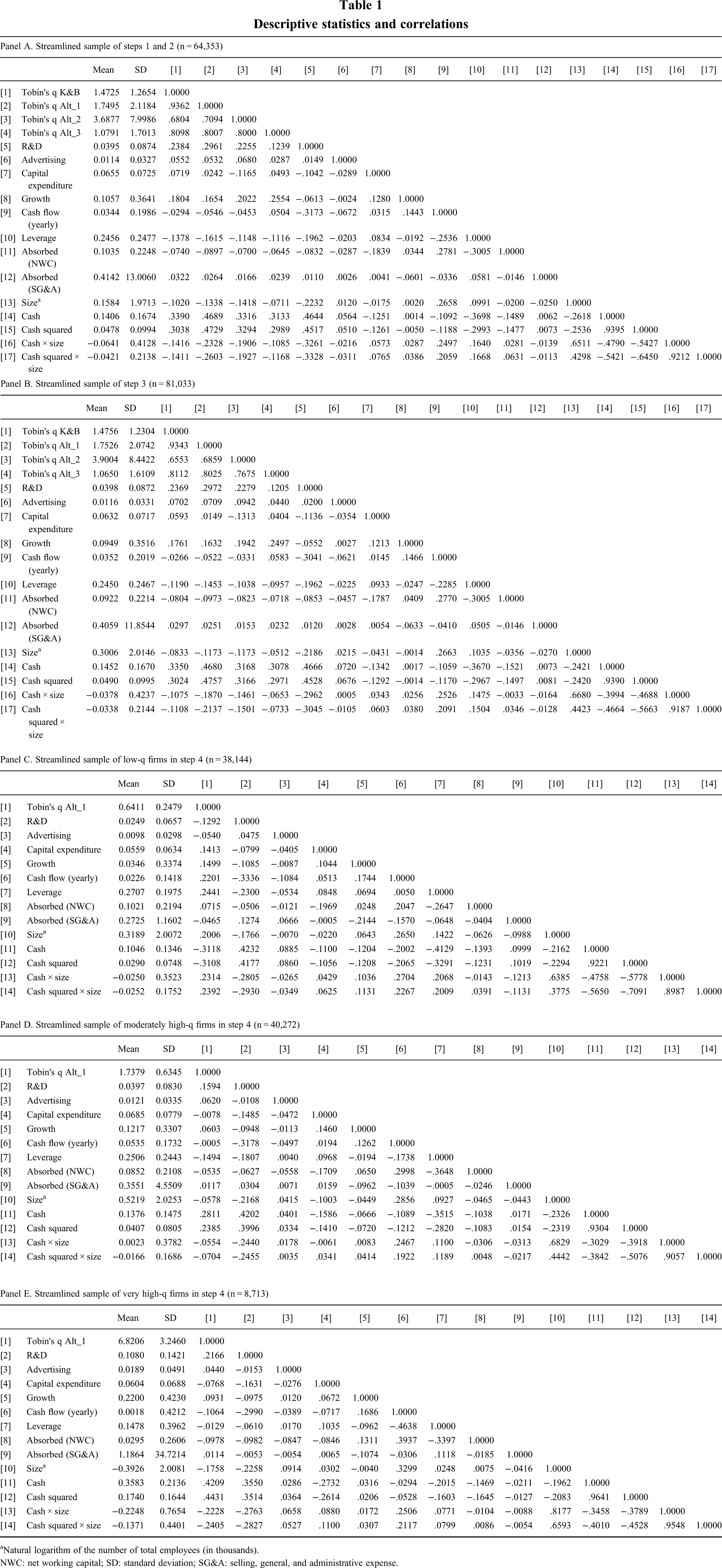
Natural logarithm of the number of total employees (in thousands).
NWC: net working capital; SD: standard deviation; SG&A: selling, general, and administrative expense.
Table 2 provides the step 1 re-examination results of the four nested regression models of Kim and Bettis (2014: 2060, 2061) alongside their original results: model (1) contains only control variables. Model (2) adds cash. Model (3) adds cash squared to test hypothesis 1. Model (4.1) adds the interaction term between cash and size to test hypothesis 2. On top of that, model (4.2) follows Kim and Bettis (2014: 2061) who explain that they “also checked the interaction between size and cash squared,” and thus adds the corresponding interaction term (see Haans, Pieters, & He, 2016).
Regression results. Literal reproduction (step 1)
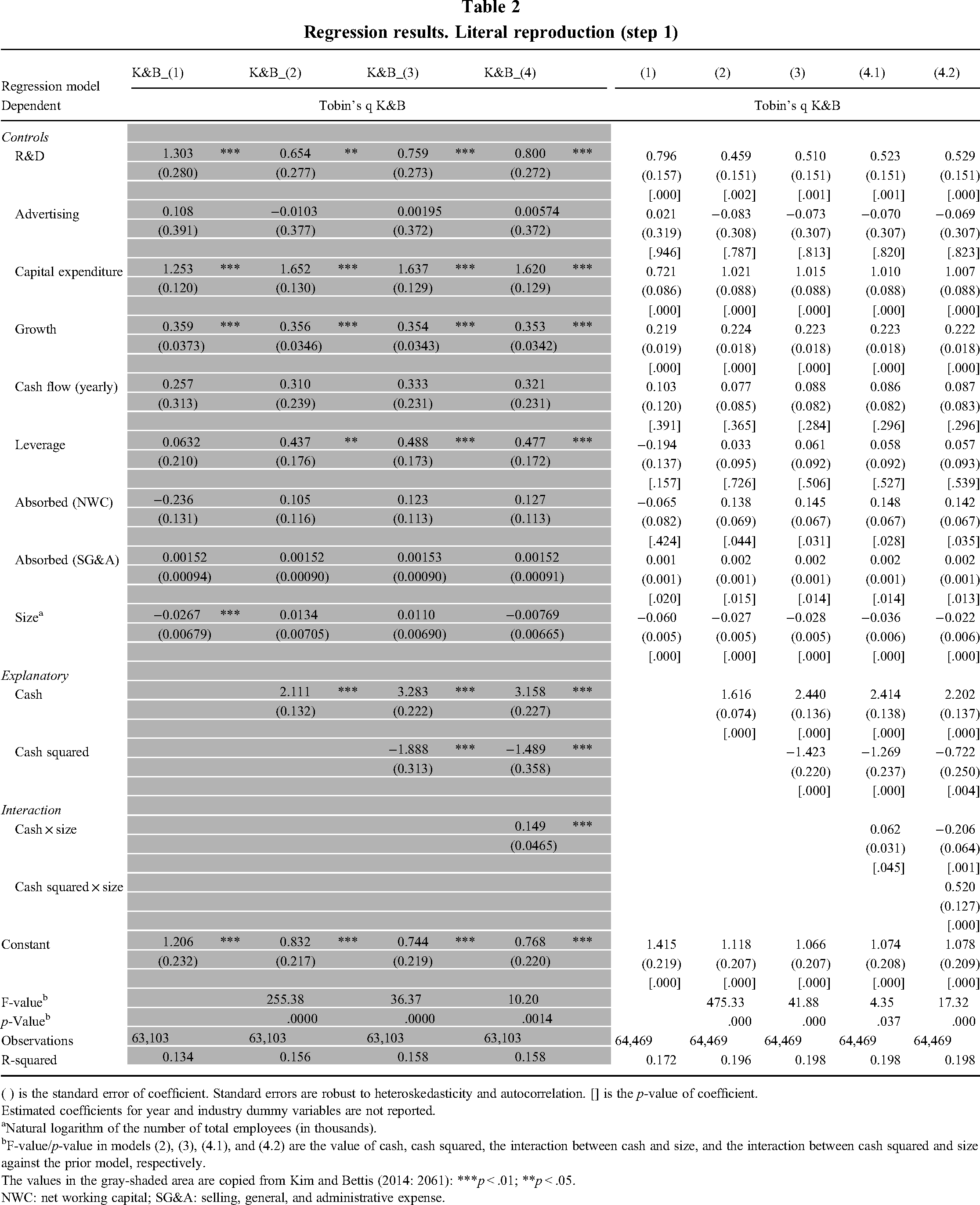
( ) is the standard error of coefficient. Standard errors are robust to heteroskedasticity and autocorrelation. [] is the p-value of coefficient.
Estimated coefficients for year and industry dummy variables are not reported.
Natural logarithm of the number of total employees (in thousands).
F-value/p-value in models (2), (3), (4.1), and (4.2) are the value of cash, cash squared, the interaction between cash and size, and the interaction between cash squared and size against the prior model, respectively.
The values in the gray-shaded area are copied from Kim and Bettis (2014: 2061): ***p < .01; **p < .05.
NWC: net working capital; SG&A: selling, general, and administrative expense.
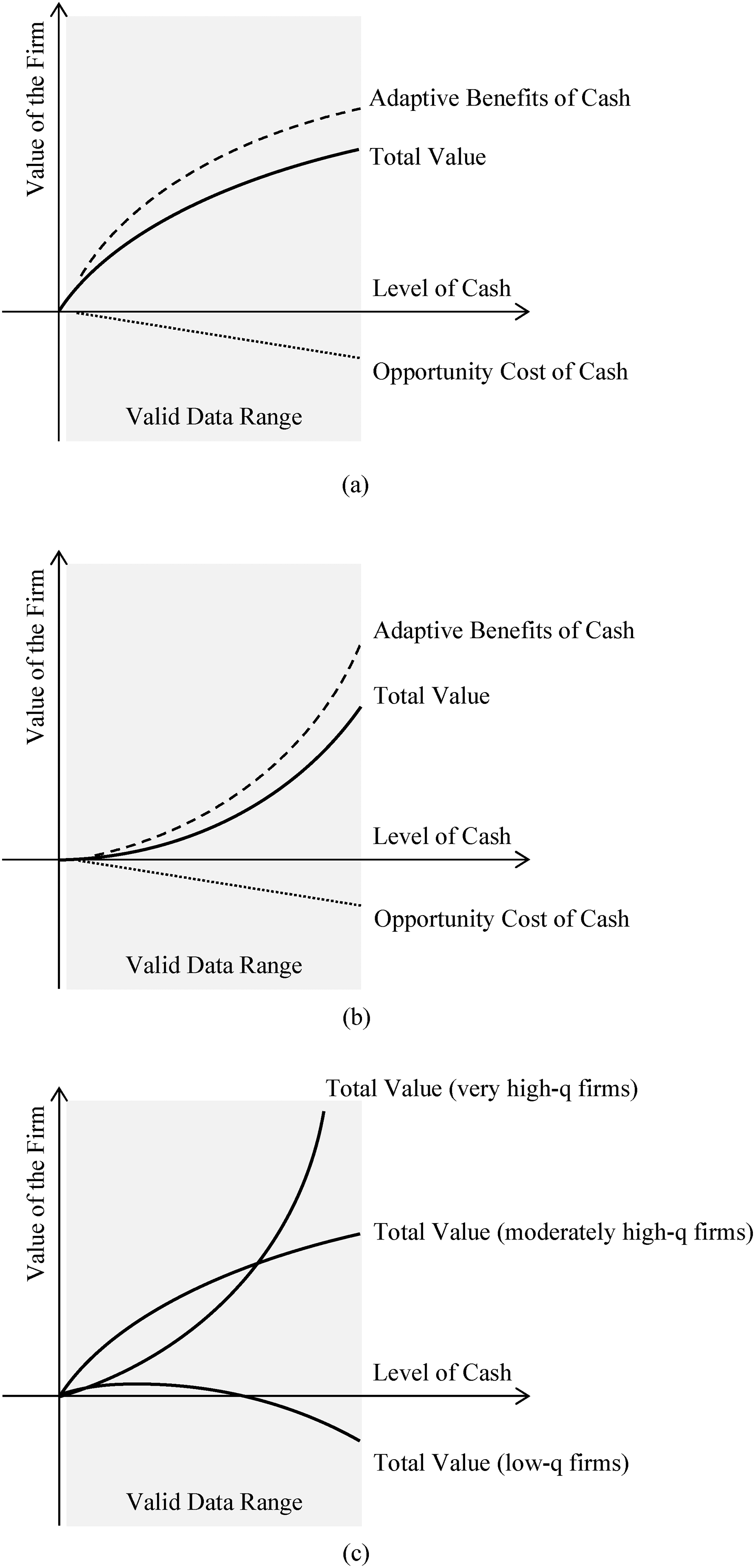
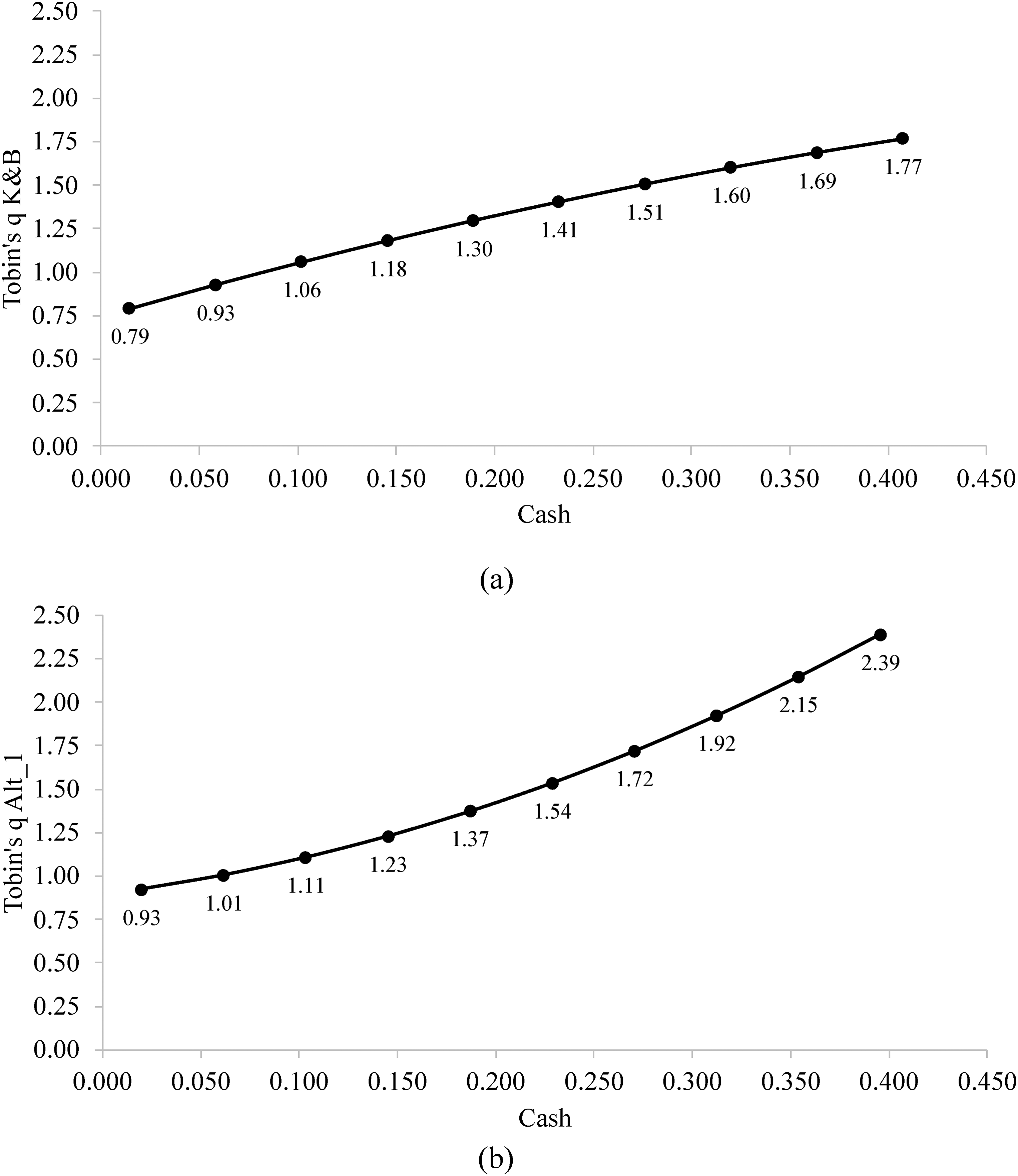
Our results using the winsorization described above fully reproduce the results of Kim and Bettis (2014) (diagram (a) of Figure 1). The cash coefficient is positive and statistically significant (p = .000) in models (2) to (4.1). The cash squared coefficient is negative and statistically significant (p = .000) in models (3) and (4.1). The interaction term between cash and size in model (4.1) is positive and statistically significant (p = .045). On top of that, the interaction term between cash squared and size in model (4.2) is positive and statistically significant (p = .000).
Re-examination results
Quasi-reproduction: Altered measurement of the dependent variable (step 2)
Building on our literal reproduction of Kim and Bettis (2014), we now alter their measurement of the dependent variable (i.e., Tobin's q) to obtain undistorted regression results. Following recommended re-examination procedures (Bettis et al., 2016b; Ethiraj et al., 2016), we leave everything else unchanged to clearly isolate the source of potential differences in results.
Tobin's q is the ratio of the market value of a firm's capital stock to its replacement costs. The classic q-theory of investment (Hayashi, 1982; Tobin, 1969) predicts that Tobin's q “perfectly summarizes a firm's investment opportunities” (Peters & Taylor, 2017: 252). In terms of measurement, Erickson and Whited (2000,: 1029) noted that while Tobin's q is observable in principle, “in practice its measurement presents numerous difficulties.” Several—often highly correlated (e.g., Chung & Pruitt, 1994)—measures of Tobin's q have therefore evolved (see Erickson & Whited, 2006). Notably, a specific Tobin's q measure may be suitable in one research setting but unsuited in another (see Erickson & Whited, 2006).
The measurement of Tobin's q in Kim and Bettis’ (2014) research setting warrants particular attention. Tobin's q is neither a pure accounting measure, such as return on assets, nor a pure financial market measure, such as total shareholder return, but a hybrid measure of firm performance (Richard, Devinney, Yip, & Johnson, 2009). While estimating its numerator (i.e., market value of a firm's capital stock) combines accounting and financial market data, estimating its denominator (i.e., replacement value of the firm's capital stock) relies on accounting data alone. Because the focal explanatory construct of Kim and Bettis (2014), that is, cash holdings, is itself a balance sheet item, there is the hazard of a problematic mathematical interrelation between cash holdings and Tobin's q in a regression model. Whether this problematic possibility materializes depends on the specific measurement of Tobin's q.
Bearing in mind that the overall research interest is in changes in cash holdings, it is helpful to emphasize that the following relationships hold by definition: All other assets being equal, an increase (a decrease) in cash holdings causes an identical increase (decrease) in total assets. Furthermore, all other assets being equal, an increase (a decrease) in cash holdings causes an identical increase (decrease) in the firm's market value coupled with an adjustment by shareholders. Due to Kim and Bettis’ (2014) chosen measurement of Tobin's q, cash holdings are not only part of their independent variable, but also part of their dependent variable's numerator (i.e., a firm's market value) and denominator (i.e., total assets). We can now demonstrate how a change in the independent variable's numerator (i.e., cash holdings) unintendedly affects the dependent variable's quotient. It is an algebraic rule that adding a positive number to both the numerator and denominator of a positive quotient causes the resulting quotient to be closer to 1 than is the starting quotient. Two inferences follow from this rule. First, adding a positive number c to a and b of a starting quotient
In the light of this algebra, the following two cases illustrate how the Tobin's q measure chosen by Kim and Bettis (2014) distorts their regression results. In both cases, a firm with initial total assets (AT) of $1,000 m raises $200 m ($100 m long-term debt and $100 m common stock) to increase its cash holdings, leaving all other decisions unchanged.
2
The capital market will incorporate this information and the firm's share price will adjust accordingly (see Malkiel, 2003).
3
The firm's book value leverage ratio (LR) of 50% remains unchanged. Case 1: The firm's initial Tobin's q is 0.80. Thus, the market value of the firm is $800 m. The firm's initial common stock (PRCC_C × CSHO) is $300 m. We further assume that the capital market disapproves of the firm's decision to raise the additional $200 m, resulting in a 5% drop in the share price. How does the firm's Tobin's q change? The book value of long-term debt (DLTT) increases to $600 m ($500 m + $100 m). The market value of common stock increases only to $385 m ($300 m – $15 m + $100 m). Total assets increase to $1,200 m ($1,000 m + $200 m). The firm's new Tobin's q is 0.82 ([$385 m + $600 m] / $1,200 m). Following Kim and Bettis’ (2014) measurement, the firm's Tobin's q therefore increases from 0.80 to 0.82. In sum, Tobin's q increases by 2.60%, although the share price decreased by 5%. While this positive change in Tobin's q is mathematically correct, it does not reflect the negative change in firm value. Here, the Tobin's q measure chosen by Kim and Bettis (2014) overestimates the performance effect of increased cash holdings.
Case 2: The firm's initial Tobin's q is 1.40. Thus, the market value of the firm is $1,400 m. The firm's initial common stock is $900 m. We further assume that this time the capital market approves of the firm's decision to raise the additional $200 m, resulting in a 5% rise in the share price. How does the firm's Tobin's q change? The book value of long-term debt again increases to $600 m. The market value of common stock increases to $1,045 m ($900 m + $45 m + $100 m). Total assets again increase to $1,200 m. The firm's new Tobin's q is 1.37 ([$1,045 m + $600 m] / $1,200 m). Following Kim and Bettis’ (2014) measurement, the firm's Tobin's q therefore decreases from 1.40 to 1.37. In sum, Tobin's q decreases by 2.08%, although the share price increased by 5%. While this negative change in Tobin's q is mathematically correct, it does not reflect the positive change in firm value. Here, the Tobin's q measure chosen by Kim and Bettis (2014) underestimates the performance effect of increased cash holdings.
We can infer from both cases that the Tobin's q measure chosen by Kim and Bettis (2014) reflects changes in firm value caused by changes in cash holdings in a distorted manner. It is important to remember the algebraic rule introduced earlier: adding a positive number to the numerator and denominator of a positive quotient causes the resulting quotient to be closer to 1 than is the starting quotient. As a consequence, the Tobin's q measure chosen by Kim and Bettis (2014) overestimates (underestimates) the performance effect of increased cash holdings if Tobin's q is below (above) 1. Their regression model configuration is, thus, prone to spurious effects causing systematically distorted regression results. In sum, while Kim and Bettis’ (2014) Tobin's q measure itself is not flawed, its use in the context of their study is problematic.
A Tobin's q measure that does not include cash holdings in the numerator and denominator will eliminate the spurious effects explicated above, because changes in the independent variable's numerator (i.e., cash holdings) will no longer unintendedly affect the dependent variable's quotient. Therefore, a Tobin's q measure that does not include cash holdings in the numerator and denominator is appropriate. For the purpose of clarification, the market value of cash holdings consists of these cash holdings (which are accounting data and found in the balance sheet) plus an adjustment by the capital market that can be positive or negative. Shareholders may favor relatively low or relatively large cash holdings for specific companies. The stock price will account for the market value of cash holdings. Hence, we are able to infer the value that the stock market attributes to different cash holdings. Due to this adjustment by the stock market, all other assets being equal, an increase (a decrease) in cash holdings does not necessarily cause an identical increase (decrease) in the firm's market value. In contrast, all other assets being equal, an increase (a decrease) in cash holdings always causes an identical increase (decrease) in total assets.
Methods
Just like previous research that has adjusted Tobin's q (Erickson & Whited, 2012; Peters & Taylor, 2017), we now make use of an altered Tobin's q measure that does not include cash holdings in the numerator and denominator. 4
In models (5) to (7.2), we alter Kim and Bettis’ (2014) measurement of Tobin's q by subtracting cash and short-term investments (CHE) from the numerator and denominator (see Erickson & Whited, 2012: 1294). Tobin's q is then calculated as the firm's market value minus cash holdings divided by firm's total assets minus cash holdings. We label this alternative Tobin's q measure Tobin's q Alt_1. All other regression model specifications remain unchanged.
Results
Panel A of Table 1 provides the descriptive statistics and the correlation matrix for the variables in our step 2 re-examination sample. Table 3 provides the step 2 re-examination results of the three nested cash regression models of Kim and Bettis (2014). Model (5) contains the control variables and cash. Model (6) adds cash squared to test hypothesis 1. Model (7.1) adds the interaction term between cash and size to test hypothesis 2. On top of that, model (7.2) adds again the interaction term between cash squared and size (see Haans et al., 2016) to further check hypothesis 2.
Regression results. Quasi-reproduction: Altered measurement of the dependent variable (step 2)
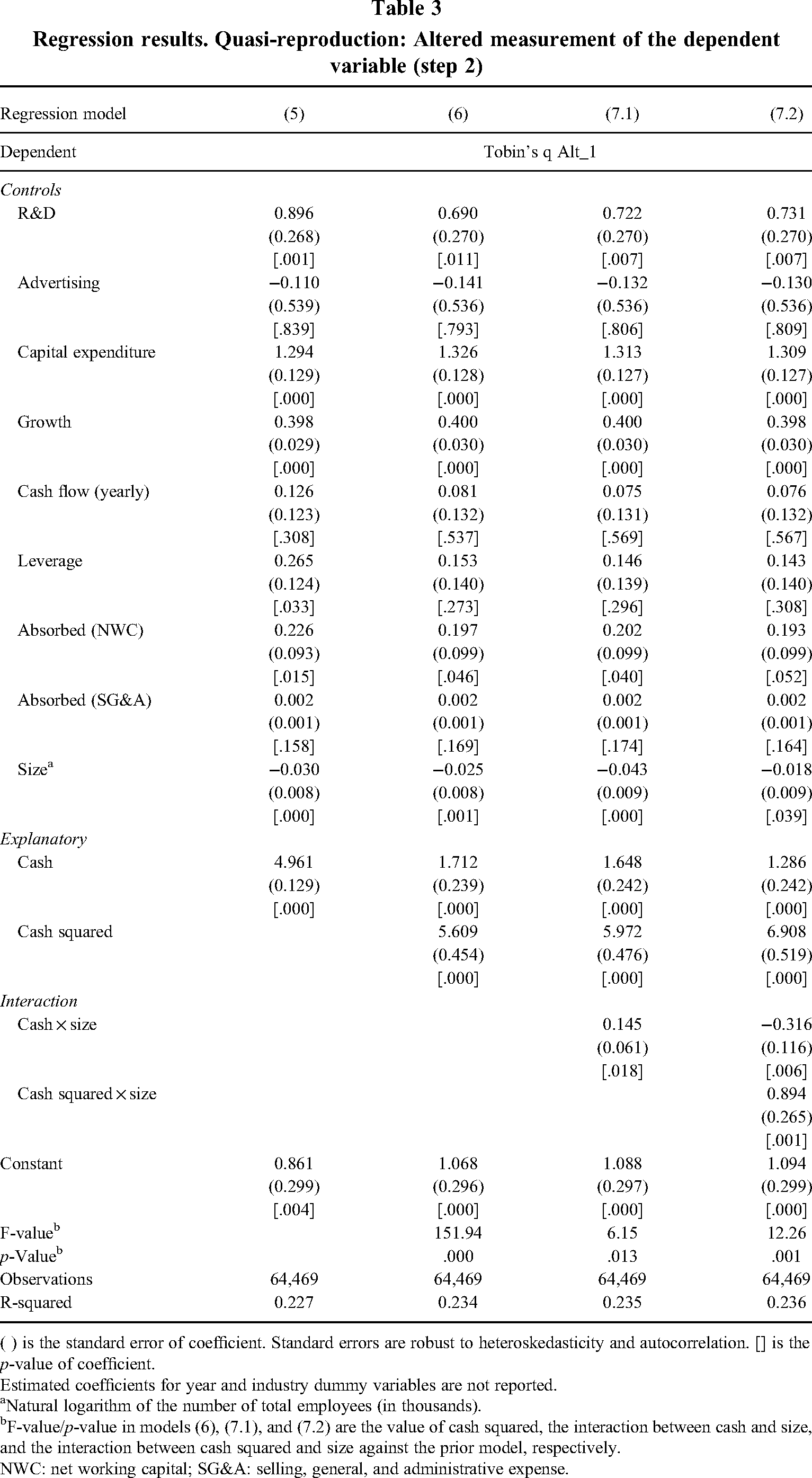
( ) is the standard error of coefficient. Standard errors are robust to heteroskedasticity and autocorrelation. [] is the p-value of coefficient.
Estimated coefficients for year and industry dummy variables are not reported.
Natural logarithm of the number of total employees (in thousands).
F-value/p-value in models (6), (7.1), and (7.2) are the value of cash squared, the interaction between cash and size, and the interaction between cash squared and size against the prior model, respectively.
NWC: net working capital; SG&A: selling, general, and administrative expense.
Consistent with the original study, the cash coefficient is positive and statistically significant (p = .000) in model (5). The cash coefficient is also positive and statistically significant (p = .000) in model (6). In contrast to the original study, the cash squared coefficient is no longer negative but positive and strongly significant at 5.609 (p = .000) in model (6). Instead of an inverted U-shape (i.e., negative squared term) as hypothesized by Kim and Bettis (2014), we thus find a U-shaped (i.e., positive squared term) relationship between cash stock and firm value (diagram (b) of Figure 1). As shown in panel A of Table 1, the correlation between Tobin's q Alt_1 and Tobin's q K&B, which denotes the measure used by Kim and Bettis (2014), is very high (r = .9362, p = .000). The fact that we find very different results for the cash squared coefficient despite this very high correlation corroborates our argument that the regression model configuration of Kim and Bettis (2014) is prone to spurious effects causing systematically distorted regression results. In sum, hypothesis 1 of Kim and Bettis (2014) is no longer supported.
With respect to hypothesis 2 of Kim and Bettis (2014), the interaction term between cash and size in model (7.1) is again positive and statistically significant (p = .018). On top of that, the interaction term between cash squared and size in model (7.2) is positive and statistically significant (p = .001). Thus, hypothesis 2 of Kim and Bettis (2014) is supported. We obtain similar results when approximating firm size via two alternative proxies, namely total assets (log) and total revenues (log) (e.g., Josefy, Kuban, Ireland, & Hitt, 2015).
Quasi-replication: Extended sample period (step 3)
In our third step, we examine how generalizable our inferences from step 2 are in terms of time (Zhao & Murrell, 2016). We now make use of a larger sample which includes the observations of Kim and Bettis (2014) and extends their time frame.
Methods
The sample period of Kim and Bettis (2014) ranges from 1988 to 2009, resulting in 63,103 firm-year observations. Our extended sample period using the Tobin's q Alt_1 measure also starts in 1988 but ends only in 2019. Compared to models (5) to (7.2), our extended sample period in models (8) to (10.2) results in a 35% larger sample, adding over 22,000 observations. All other regression model specifications in step 3 are kept unchanged in comparison with step 2.
Results
Panel B of Table 1 provides the descriptive statistics and the correlation matrix for the variables in our step 3 re-examination sample. Table 4 provides the step 3 re-examination results of the three nested cash regression models of Kim and Bettis (2014). Model (8) contains the control variables and cash. Model (9) adds cash squared to test hypothesis 1. Model (10.1) adds the interaction term between cash and size to test hypothesis 2. Finally, model (10.2) adds the interaction term between cash squared and size (see Haans et al., 2016) again to further check hypothesis 2.
Regression results. Quasi-replication: Extended sample period (step 3)
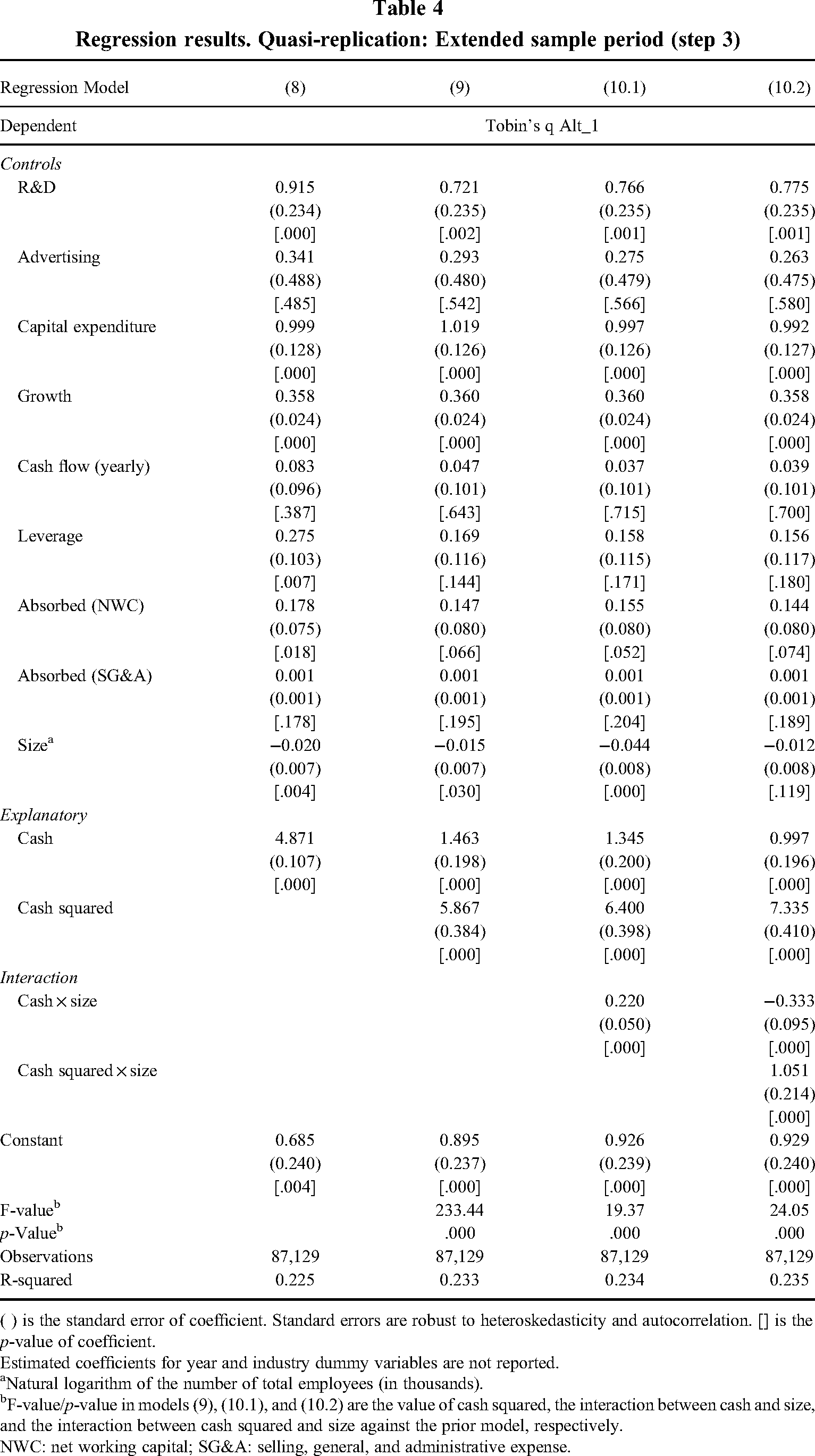
( ) is the standard error of coefficient. Standard errors are robust to heteroskedasticity and autocorrelation. [] is the p-value of coefficient.
Estimated coefficients for year and industry dummy variables are not reported.
Natural logarithm of the number of total employees (in thousands).
F-value/p-value in models (9), (10.1), and (10.2) are the value of cash squared, the interaction between cash and size, and the interaction between cash squared and size against the prior model, respectively.
NWC: net working capital; SG&A: selling, general, and administrative expense.
There are no substantial differences in the results of models (8) to (10.2) compared to their counterpart models in step 2. Hence, our step 3 re-examination results confirm our inferences of step 2. While hypothesis 1 of Kim and Bettis (2014) is again no longer supported, their hypothesis 2 remains supported in the extended sample period.
As in step 2, the coefficients of cash and cash squared in the step 3 regression model (9) cause the function's global minimum to be at a calculated cash stock below zero. As a firm's cash stock cannot be negative, each minimum is located outside the possible data range. From a purely numerical point of view, more cash constantly drives firm value at increasing rates for cash stocks between 0% and 100%. Note, however, that in our step 3 sample, 80% of the firm-year observations have a cash stock between 0.77% and 39.35%. Therefore, from a practical point of view, we can only confidently conclude that more cash drives firm value at increasing rates in this valid data range. In this regard, we concur with Kim and Bettis (2014: 2056, 2060) that estimations “near the ends of the sample regarding cash holdings have wide confidence intervals” and that estimations “are meaningless beyond what is justified by the presence of adequate data as we move toward extreme values.”
Quasi-replication: Split of sample (step 4)
In our final step, we address our third concern. Kim and Bettis (2014) did not specifically explore the role of a firm's available investment opportunities in their testing of the cash–performance relationship. In other words, they did not differentiate between firms with low investment opportunities and firms with high investment opportunities. Correspondingly, our previous regression results with regard to hypothesis 1 of Kim and Bettis (2014) also do not make this differentiation. In fact, this might explain our results in steps 2 and 3 with regard to hypothesis 1 of Kim and Bettis (2014), namely that we find the cash squared coefficient to be no longer negative but positive and strongly significant (see models (6) and (9)). This convex relationship between cash stock and firm value could, for example, be driven by firms with very high investment opportunities.
We conjecture that the benefits of large cash holdings may largely rest on a firm's level of investment opportunities. Only if a firm possesses valuable investment opportunities can cash unfold its quality of enabling a firm to seize value-creating projects and transitions swiftly. Hence, only a high level of investment opportunities may fully facilitate the adaptive benefits of cash put forth by Kim and Bettis (2014). Thus, the cash–performance relationship could differ substantially for three types of firms, namely firms with low investment opportunities, firms with moderately high investment opportunities, and firms with very high investment opportunities.
Methods
To consider a firm's level of investment opportunities in our testing of the cash–performance relationship, we split our sample into three subsamples. We use Tobin's q to do so (Szewczyk, Tsetsekos, & Zantout, 1996), as the classic q-theory of investment (Hayashi, 1982; Tobin, 1969) predicts that Tobin's q “perfectly summarizes a firm's investment opportunities” (Peters & Taylor, 2017: 252). Indeed, Tobin's q is “an increasing function of the quality of a firm's current and anticipated projects under existing management” (Lang, Stulz, & Walkling, 1989: 138).
Of course, we need to specify two appropriate thresholds at which we split the sample (see Hansen, 2000). The first threshold presents the value of Tobin's q at which to separate firms with low investment opportunities from firms with moderately high investment opportunities. We set this threshold to one (Lang et al., 1989; Szewczyk et al., 1996), because at this value of Tobin's q the market value of a firm's capital stock (i.e., assets) equals its replacement costs. The second threshold presents the value of Tobin's q at which to separate firms with moderately high investment opportunities from firms with very high investment opportunities. We set this threshold to the top decile, which means that the third subsample consists of those 10% firms that have the highest Tobin's q values in our sample. Taken together, our first subsample consists of low-q firms, our second subsample consists of moderately high-q firms, and our third subsample consists of very high-q firms (Lang et al., 1989; Szewczyk et al., 1996).
Because our concern that Kim and Bettis (2014) did not specifically consider a firm's level of investment opportunities only applies to testing their hypothesis 1, that is, the main cash–performance relationship, we do not revisit their hypothesis 2 in this step. Hence, we omit regression models that are designed to test the interaction of cash holdings with firm size. All other regression model specifications in step 4 are kept unchanged in comparison with step 3.
Results
Panels C, D, and E of Table 1 provide the descriptive statistics and the correlation matrix for the variables in our first (i.e., low-q firms), second (i.e., moderately high-q firms), and third subsamples (i.e., very high-q firms), respectively. For each of the three subsamples, Table 5 provides the step 4 re-examination results of the two nested cash regression models of Kim and Bettis (2014) that test their hypothesis 1, that is, the main cash–performance relationship.
Regression results. Quasi-replication: Sample split (step 4)
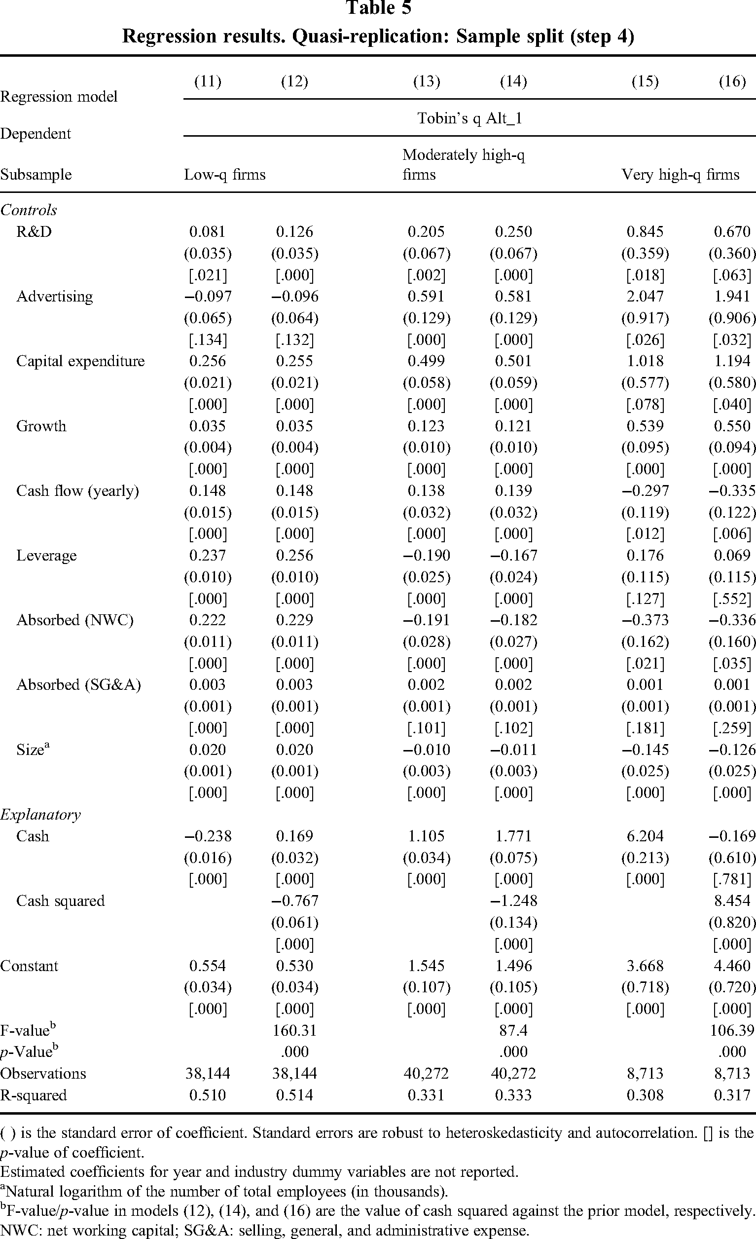
( ) is the standard error of coefficient. Standard errors are robust to heteroskedasticity and autocorrelation. [] is the p-value of coefficient.
Estimated coefficients for year and industry dummy variables are not reported.
Natural logarithm of the number of total employees (in thousands).
F-value/p-value in models (12), (14), and (16) are the value of cash squared against the prior model, respectively.
NWC: net working capital; SG&A: selling, general, and administrative expense.
In contrast to our main results reported previously, the cash coefficient is negative and statistically significant (p = .000) in model (11), which tests the linear cash–performance relationship for low-q firms. Model (12) adds cash squared. The cash coefficient is positive and statistically significant (p = .000) in model (12), and the cash squared coefficient is negative and statistically significant (p = .000) in model (12). Hence, we find that the cash–performance relationship for low-q firms takes the form of a quadratic function with a positive original term and a negative squared term, that is, an inverted U-shape.
Models (13) and (14) test the linear and quadratic cash–performance relationship, respectively, for moderately high-q firms. In contrast to model (11), the cash coefficient is positive and statistically significant (p = .000) in model (13). Similar to model (12), the cash coefficient is positive and statistically significant (p = .000), and the cash squared coefficient is negative and statistically significant (p = .000) in model (14). Hence, we find that the cash–performance relationship for moderately high-q firms also takes the form of an inverted U-shape. However, the turning point (i.e., the calculated optimal point of cash holdings) is very different for low-q firms and for moderately high-q firms. For low-q firms, the turning point is at a cash level of about 11%. For moderately high-q firms, the turning point is at a cash level of about 71%. The latter is similar to the turning point of about 89% reported by Kim and Bettis (2014: 2060). Because 80% of the firm-year observations in our first subsample have a cash stock between 0.56% and 27.31%, the turning point at a cash level of about 11% in case of low-q firms is located well inside the valid data range. As in the sample of Kim and Bettis (2014), this is not the case for moderately high-q firms. Because 80% of the firm-year observations in our second subsample have a cash stock between 0.89% and 34.81%, the turning point at a cash level of about 71% in case of moderately high-q firms is located outside the valid data range. We are thus hesitant to make strong inferences about whether this turning point may have practical relevance.
Models (15) and (16) test the linear and quadratic cash–performance relationship, respectively, for very high-q firms. The cash coefficient is positive and statistically significant (p = .000) in model (15). In contrast to Models (12) and (14), the cash squared coefficient is positive and statistically significant (p = .000) in model (16). Hence, we find that the cash–performance relationship for very high-q firms takes a convex shape. Compared to the cash squared coefficient in case of low-q firms and moderately high-q firms, this is a variant of what Haans et al. (2016: 1188) called a “shape-flip.”
Our step 4 results can be summarized as follows. In our first subsample (low-q firms), we find decreasing marginal returns of cash that turn negative for medium and large cash holdings. In our second subsample (moderately high-q firms), we find decreasing marginal returns of cash that remain positive for medium and large cash holdings. In our third subsample (very high-q firms), we find increasing marginal returns of cash. These results are visualized in Figure 1, diagram (c).
We split the sample in this step according to Tobin's q because it can be interpreted as the amount of future investment opportunities available to a firm. The results suggest that increasing returns to cash exist only for those firms that have a very high Tobin's q, that is, are judged by the capital markets to have very high investment opportunities. Since this reasoning is, however, somewhat circular given that Tobin's q is also our dependent variable, we performed additional analyses. In these analyses, we split the sample according to alternative variables that we also consider indicative of firms’ investment opportunities.
In our first additional analysis, we instead split our sample by the position of a firm's product portfolio on the product life cycle. We use data from the Hoberg and Maksimovic (2023) data library to measure firms’ product life cycle stages. Following the suggested four-stage product life cycle conceptualization of Abernathy and Utterback (1978), Hoberg and Maksimovic (2022) use computational linguistic methods applied to firms’ 10-K statements to compute a four-element vector to capture the exposure of firms’ product portfolios to each life cycle stage. We build on this measure to identify a firm's highest exposure to one of the four product life cycle stages and assign the firm-year observations to related subsamples. The four stages are (Hoberg & Maksimovic, 2022, 2023): product development (i.e., product innovation), process optimization (i.e., process innovation), product maturity, and product decline. We expect that firms positioned in the first stage (i.e., product development) exhibit the highest level of investment opportunities and, thus, benefit the most from large cash holdings.
In our second additional analysis, we instead split our sample by firm age. To measure firm age, we follow prior work (e.g., DesJardine, Bansal, & Yang, 2019) and determine the difference between the focal year and the first year the firm was covered by COMPUSTAT. We split our sample into three subsamples. The first subsample comprises those firms that are in the lowest decile of firm age (i.e., the youngest firms). Correspondingly, the third subsample comprises those firms that are in the highest decile of firm age (i.e., the oldest firms). Those firms that lie in between fall into the second subsample. We expect the youngest firms to exhibit the highest level of relative investment opportunities and, thus, benefit the most from large cash holdings.
In both analyses, we find indicative support for the idea that companies with high (low) investment opportunities profit the most (least) from cash. With regard to splitting our sample by a firm's product life cycle, the left-hand side of Table 6 provides the replication results of the two nested cash regression models of Kim and Bettis (2014) that test their hypothesis 1, that is, the main cash–performance relationship, for the first and last subsample. In model (18), the cash coefficient is positive and statistically significant (β = 3.831; p = .000) and the cash squared coefficient is positive and statistically significant (β = 4.973; p = .000). Thus, we find increasing marginal returns of cash for firms in the first stage (i.e., product development). In model (20), the cash coefficient is positive and statistically significant (β = 4.614; p = .001) and the cash squared coefficient is negative and statistically significant (β = −6.229; p = .012). Thus, we find decreasing marginal returns of cash for firms in the last stage (i.e., product decline).
Regression results. Quasi-replication: Sample splits (additional analyses of step 4)
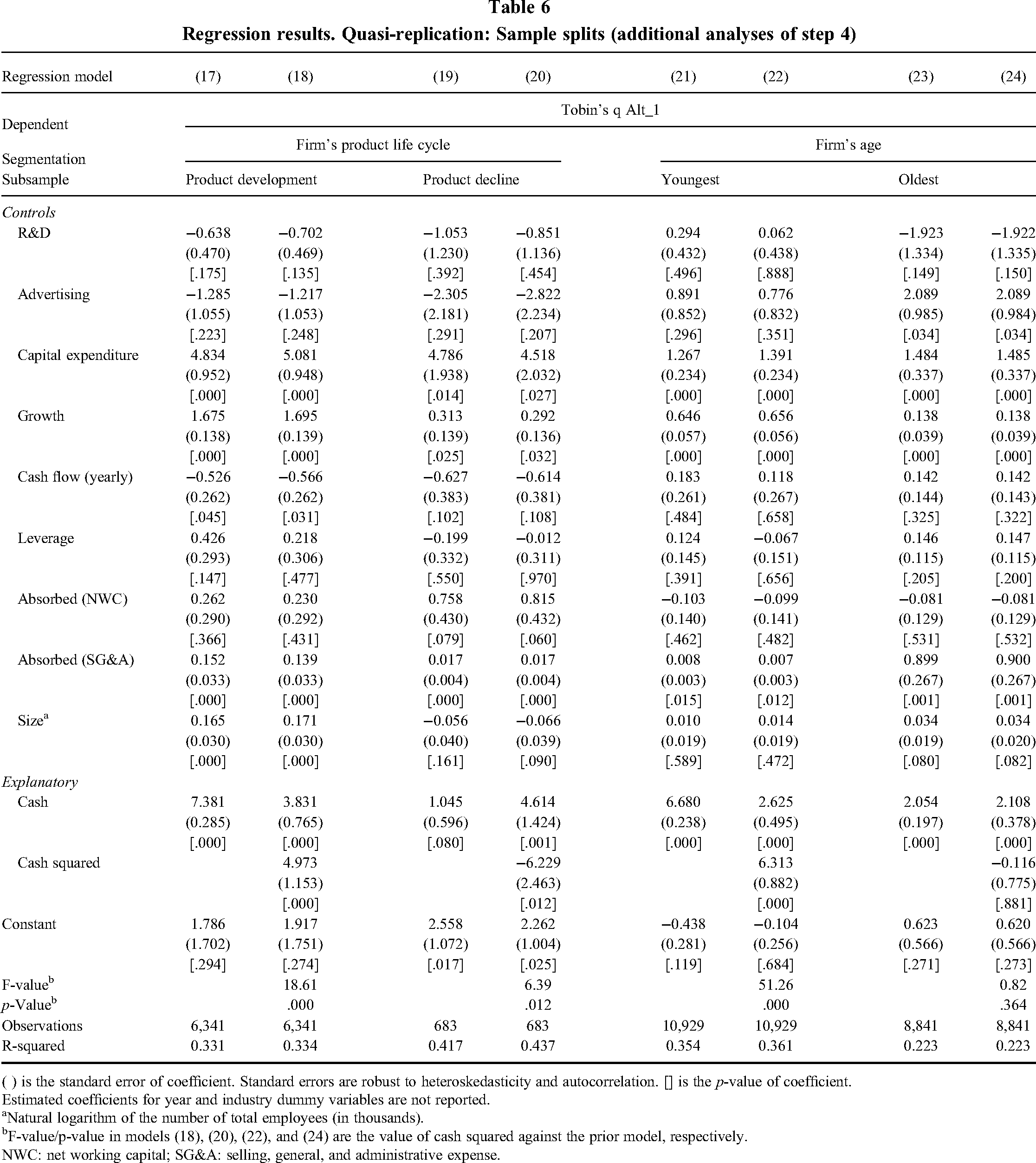
( ) is the standard error of coefficient. Standard errors are robust to heteroskedasticity and autocorrelation. [] is the p-value of coefficient.
Estimated coefficients for year and industry dummy variables are not reported.
Natural logarithm of the number of total employees (in thousands).
F-value/p-value in models (18), (20), (22), and (24) are the value of cash squared against the prior model, respectively.
NWC: net working capital; SG&A: selling, general, and administrative expense.
With regard to splitting our sample by firm age, the right-hand side of Table 6 provides the replication results of the two nested cash regression models of Kim and Bettis (2014) that test their hypothesis 1, that is, the main cash–performance relationship, for the first and last subsample. In model (22), the cash coefficient is positive and statistically significant (β = 2.625; p = .000) and the cash squared coefficient is positive and statistically significant (β = 6.313; p = .000). Thus, we find increasing marginal returns of cash for the youngest firms in the sample. In model (24), the cash coefficient is positive and statistically significant (β = 2.108; p = .000) and the cash squared coefficient is negative and not statistically significant (β = −0.116; p = .881). Thus, we do not find increasing marginal returns of cash for the oldest firms in the sample.
Importantly, we highlight that our inferences are tentative since further unreported analyses—for example, splitting the sample by firms’ R&D intensity (e.g., Ye, Yu, & Nason, 2021) or by high-tech versus low-tech industries (e.g., Gupta, Crilly, & Greckhamer, 2020; Hecker, 1999)—fairly consistently showed increasing returns to cash across different segmentations of our data.
Robustness checks
To ensure that our results are robust to alternative explanations of the cash–performance relationship, we conducted a battery of robustness checks. All results are available upon request.
Alternative measures of Tobin's q
In order to ensure that our replication results are not driven by any unnoticed peculiarities of our altered Tobin's q measure, we reran our steps 3 and 4 regression models with two additional Tobin's q measures that also do not include cash holdings in the numerator and denominator.
On the one hand, we employ the “literature's standard” Tobin's q measure (Peters & Taylor, 2017: 256), which is used, for example, by Erickson and Whited (2012). Here, we measure the numerator of the Tobin's q ratio as “the market value of outstanding equity [PRCC_F × CSHO], plus the book value of debt [DLTT × DLC], minus the firm's current assets [ACT], which include cash, inventory, and marketable securities” (Peters & Taylor, 2017: 256). We measure the denominator of the Tobin's q ratio as “the book value of property, plant, and equipment [PPEGT]” (Peters & Taylor, 2017: 256). We label this alternative Tobin's q measure Tobin's q Alt_2.
On the other hand, we employ Peters and Taylor's (2017) more elaborate measure of Tobin's q (e.g., Hope & Lu, 2020), which accounts for the replacement cost not only of physical capital but also of intangible capital. Peters and Taylor (2017: 252) therefore call it “total q”. This measure is calculated like the Tobin's q Alt_2 measure with the difference that the replacement cost of intangible capital is added to the replacement cost of physical capital in the denominator. A firm's intangible capital is defined as “the sum of the firm's externally purchased and internally created intangible capital” (Peters & Taylor, 2017: 252, 256) and the respective data can be retrieved from Wharton Research Data Services. We label this Tobin's q measure Tobin's q Alt_3.
In sum, cash holdings are not part of the dependent variable's numerator and denominator in all three cases (i.e., Tobin's q Alt_1, Tobin's q Alt_2, and Tobin's q Alt_3), allowing undistorted regression results. As shown in Table 1, the three alternative measures are highly correlated with the Tobin's q measure chosen by Kim and Bettis (2014). The correlations in our extended sample (see panel B of Table 1) range between .6553 (p = .000) and .9343 (p = .000). 5
The results are as follows. First, there are no significant changes in terms of interpreting our step 3 results with regard to hypothesis 1 of Kim and Bettis (2014): It is again no longer supported. When testing the quadratic cash–performance relationship and using Tobin's q Alt_2, the cash coefficient is again positive and statistically significant (β = 2.979; p = .001) and the cash squared coefficient is again positive and statistically significant (β = 9.448; p = .000). When testing the quadratic cash–performance relationship and using Tobin's q Alt_3, the cash coefficient is again positive and statistically significant (β = 1.958; p = .000) and the cash squared coefficient is again positive and statistically significant (β = 0.963; p = .000).
Second, we now find only mixed support for hypothesis 2 of Kim and Bettis (2014). When checking the robustness of model (10.1) using Tobin's q Alt_2, the interaction term between cash and size is negative but not statistically significant (β = −0.147; p = .470). And when checking the robustness of model (10.2), the interaction term between cash squared and size is again positive but no longer statistically significant (β = 0.290; p = .727). When checking the robustness of model (10.1) using Tobin's q Alt_3, the interaction term between cash and size is again positive and statistically significant (β = 0.213; p = .000). And when checking the robustness of model (10.2), the interaction term between cash squared and size is again positive and statistically significant (β = 0.484; p = .001). Taken together, hypothesis 2 of Kim and Bettis (2014) is no longer supported when we use Tobin's q Alt_2, but it is again supported when we use Tobin's q Alt_3. This may indicate a weakly positive cash–size interaction effect.
Third, there are no significant changes in terms of interpreting our step 4 results. When testing the quadratic cash–performance relationship for low-q firms and using either Tobin's q Alt_2 or Tobin's q Alt_3, the cash coefficient is again positive and statistically significant (β = 0.532; p = .000 and β = 0.257; p = .000, respectively) and the cash squared coefficient is again negative and statistically significant (β = −2.132; p = .000 and β = −0.595; p = .000, respectively). When testing the quadratic cash–performance relationship for moderately high-q firms using either Tobin's q Alt_2 or Tobin's q Alt_3, the cash coefficient is again positive and statistically significant (β = 2.999; p = .000 and β = 0.636; p = .000, respectively) and the cash squared coefficient is again negative and statistically significant (β = −1.824; p = .000 and β = −0.537; p = .000, respectively). When testing the quadratic cash–performance relationship for very high-q firms using either Tobin's q Alt_2 or Tobin's q Alt_3, the cash squared coefficient is again positive and statistically significant (β = 10.260; p = .019 and β = 1.289; p = .058, respectively).
Alternative winsorization and trimming
To ensure that any confounding effects of unnoticed outliers do not drive our replication results, we reran our steps 3 and 4 regression models with alternative procedures for removing outliers. Recall that, in our main regression models, we winsorize the dependent variable, that is, Tobin's q, and the two explanatory variables, that is, cash and size, at the bottom 1% and top 1% level (e.g., Flammer & Kacperczyk, 2019; Shan et al., 2017).
As a first robustness check in this respect, we take an even more conservative approach by conducting winsorization of the dependent variable and the two explanatory variables at the bottom and top 5% level (Flammer, Hong, & Minor, 2019). We cautiously note that such wide boundaries of winsorization may, of course, cut out valuable variation at the upper and lower end of the variable distributions. Yet, there are no significant changes in terms of interpreting our steps 3 and 4 re-examination results. When testing the quadratic cash–performance relationship of step 3, the cash coefficient is again positive and statistically significant (β = 1.932; p = .000) and the cash squared coefficient is again positive and statistically significant (β = 2.114; p = .000). Thus, hypothesis 1 of Kim and Bettis (2014) is again not supported. When checking the robustness of model (10.1), the interaction term between cash and size is again positive and statistically significant (β = 0.133; p = .000). And when checking the robustness of model (10.2), the interaction term between cash squared and size is again positive and statistically significant (β = 0.984; p = .000). Thus, hypothesis 2 of Kim and Bettis (2014) is supported again.
In further robustness checks, we conducted trimming (e.g., Bertrand, Betschinger, & Settles, 2016) instead of winsorization by excluding firm-year observations that fall in the bottom or top 1% or 5%. Again, there are no significant changes in terms of interpreting our step 3 re-examination results. With respect to our step 4 regression models, the results are predominantly similar to our main replication reported previously.
Overall, these robustness checks suggest that natural outliers do not drive our replication results. They also caution us to not treat individual companies at the upper or lower boundaries of cash levels as empirical archetypes for assessing the desirability of firms holding cash.
Alternative functional forms
We also ensured that the observed functional form is indeed quadratic and, in turn, that alternative and more complex specifications can be ruled out, such as a cubic (S-shaped) functional form. We follow prior suggestions (e.g., Arin, Minniti, Murtinu, & Spagnolo, 2022) and leverage semiparametric techniques to inspect and explore alternative specifications of curvilinear functional forms.
Specifically, we leverage the methodological innovation of binned scatterplots (e.g., Starr & Goldfarb, 2020) (binsreg command in Stata). The binned scatterplot applied to model (8) of Table 4, shown in Figure 2, partitions the x-axis (cash holdings) into bins, for each of which the mean of the dependent variable (firm performance) is calculated. A regression model for which the relationship between x and y can differ in each bin is then estimated, accounting for all control variables. Following Starr and Goldfarb's (2020) recommendations, we show a binned scatterplot with the number of bins chosen by minimizing the integrated mean squared error and confidence bands for each point, leading to 44 bins for our sample.
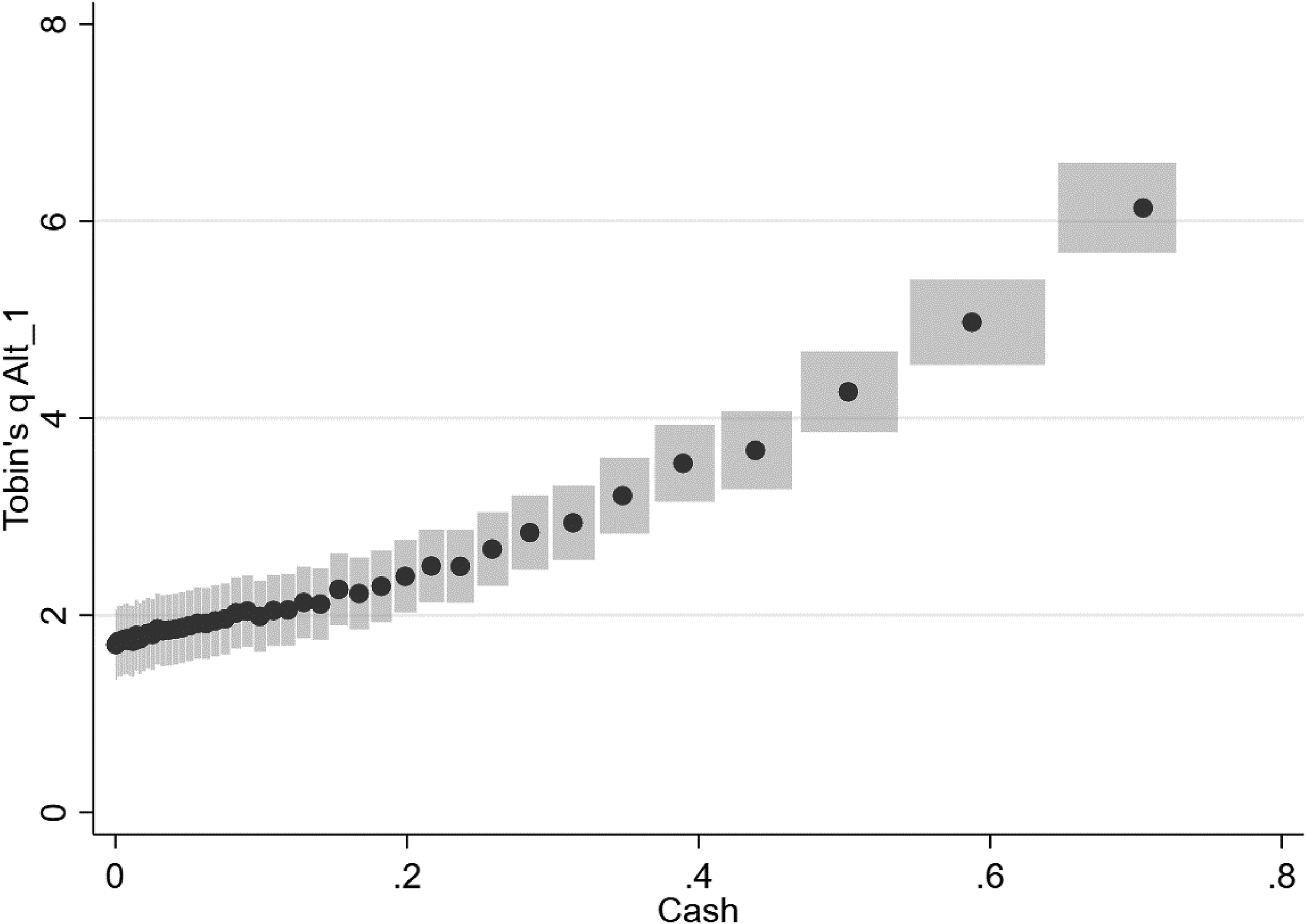
Binned scatterplot (exemplified for model 8 of Table 4)
Figure 2 shows that the effect of cash holdings is positive and even increases at higher levels. Thus, the binned scatterplot—like those created for each model specification with alternative dependent variables as per step 3—that is, Tobin's q Alt_2 and Tobin's q Alt_3—substantiates a convex functional form rather than an inverted U-shape relationship, which provides further tentative support to our main findings. Next, following Haans et al. (2016), we added a cubic term to our squared model as per step 3, that is, model (9) of Table 4. While the result for Tobin's q Alt_1 indeed tentatively indicates a cubic term that is positive and statistically significant (β = 6.764; p = .000), such a cubic term was not found to be consistently statistically significant across our models when using alternative variants of our dependent variable. For example, results for Tobin's q Alt_3 indicate that the cubic term is positive but not statistically significant (β = 0.2570; p = .827), and a likelihood ratio test confirms that the model's explanatory power does not increase by including a cubic term (chi-squared = 1.76; p = .1846). Thus, the results do not conclusively point toward a higher-order functional form. Notably, even in models that show a statistically significant effect of the cubic term, this term is positive, that is, not indicating a penalty for holding too much cash, and the squared term of cash holdings is not statistically significant, supporting a convex functional form. Thus, we conclude that a quadratic model specification—as in our main analysis—is adequate to model the cash–performance relationship.
Alternative estimation procedure
We also altered our estimation procedure. We follow Deb et al. (2017) and use a dynamic fixed effects model, including the lagged dependent variable as a control variable. Our results are qualitatively similar for step 3, indicating both a positive and statistically significant linear and squared term. Results on Tobin's q Alt_1 show a positive and statistically significant effect of the lagged dependent variable (β = 0.517; p = .000)—which is in line with Deb et al. (2017)—while both the positive and statistically significant linear (β = 0.942; p = .000) and squared term (β = 3.188; p = .000) of cash holdings persist. Our results are also qualitatively similar for the analyses from step 4. Notably, for very high-q firms, as exemplified via the uppermost decile of Tobin's q Alt_1, we find a positive and statistically significant squared term (β = 6.5570; p = .000), substantiating our main results that there is no penalty for holding high levels of cash for such firms. Moreover, although no temporal lag is desirable when using Tobin's q as a dependent variable given that it is an at least partially market-based performance measure (e.g., Richard et al., 2009), we still introduce a temporal lag of 1 year to our model. Our results are fully robust for both steps 3 and 4. For instance, when applied to model (9) of Table 4, we still can observe both a positive and statistically significant linear effect (β = 1.107; p = .000) and squared effect of cash holdings (β = 2.850; p = .000). Thus, we can confirm that the performance effects of cash holdings do not hinge on a particular temporal structure of our model specification.
Market conditions
Prior studies suggest that the performance implications of cash holdings may vary between market conditions (e.g., Deb et al., 2017; Jung, Foege, & Nüesch, 2020). As for industry contexts, our main model specification includes industry-fixed effects and year-fixed effects that account for general industry characteristics and macroeconomic events or trends (e.g., Vanacker, Forbes, Knockaert, & Manigart, 2020). Moreover, we also used industry-year fixed effects as a robustness check to further probe for potential time-varying industry trends (e.g., Flammer & Luo, 2017). Our results are fully robust, including alternative industry classifications of the focal firm's primary industry using two-digit or four-digit SIC codes as alternatives to the main models of steps 3 and 4 at the three-digit SIC level. In addition, and to more explicitly account for recessionary periods that are found to affect the value-creation potential of cash holdings (e.g., Nason & Patel, 2016), we follow Eesley, Hsu and Roberts (2014) and use data from the National Bureau of Economic Research (NBER) Business Cycle Dating Committee to measure recessions (Stock & Watson, 2010). 6 We create a recession dummy that indicates the presence or absence of three recessions in our time frame by taking the value of “1” for 1990, 2001, 2007, 2008, 2009, and “0” otherwise. Despite a surprisingly positive and statistically significant effect of the recession dummy on firm performance, our results are qualitatively similar across all main models of steps 3 and 4. For Tobin's q Alt_1 as a dependent variable, there is a positive and statistically significant effect of the recession dummy—at least in some models—on firm performance (β = 0.064; p = .001) and the positive and statistically significant linear (β = 1.461; p = .000) and squared effect (β = 5.869; p = .000) of cash holdings persist. Likewise, for very high-q firms we also observe a positive squared term of cash holdings (β = 8.469; p = .000). Overall, our evidence suggests that the debate on the desirability of cash holdings does not necessarily require a focus on specific macroeconomic trends.
Quarterly data
We probed if the use of more fine-grained, that is, quarterly, data affects our estimates. However, such data is not consistently available for our dependent and control variables needed for rigorous replication. Still, as quarterly data on cash holdings is available, we used the cash holdings lagged by one-quarter as an alternative explanatory variable to test the robustness of our results. Our results are robust for steps 3 and 4. Results on Tobin's q Alt_1 as a dependent variable show both a positive and statistically significant linear effect (β = 0.696; p = .000) and squared effect (β = 1.667; p = .000) for the effect of lagged quarterly cash holdings on firm performance.
Cohort effects and stock repurchases
We tested whether unobserved cohort effects by period drive our results. Notably, our main specifications already account for such unobserved heterogeneity of potential cohort effects by using fixed-effects models with both industry and time dummies (e.g., Arend, Patel, & Park, 2014; Hoetker & Agarwal, 2007). In addition, we want to rule out that a possible new trend toward substantial stock repurchases after the end of the timeframe of Kim and Bettis (2014), that is, after 2009, affects our results (e.g., Floyd, Li, & Skinner, 2015). Thus, we add a “past 2009 dummy” variable to our main models in steps 3 and 4 and find that our results are largely unaffected. Only for Tobin's q Alt_1 as a dependent variable, we find a positive and statistically significant effect of the “past 2009 dummy” (β = 0.084; p = .069), while our results of both a positive and statistically significant linear (β = 1.464; p = .000) and squared term of cash holdings (β = 5.866; p = .000) are robust.
Furthermore, acknowledging that the “past 2009 dummy” can be considered a rather broad control variable to capture potential confounding effects of stock repurchases, particularly as such repurchases likely vary from year to year, we add more direct controls of firms’ share repurchases. We follow prior work by Banyi, Dyl, and Kahle (2008) on the measurement of stock repurchases, take into account that there is no standard proxy for stock repurchases in scholarly literature and thus use four alternative measures of firms’ stock repurchases based on COMPUSTAT data: (1) the decrease of shares outstanding (set to zero in case of an increase), (2) purchases of common stock, (3) increases in the number of shares of treasury stock (set to zero in case of a decrease), and (4) the Fama–French changes in treasury stock, that is, the difference between purchases and sales of common and preferred stock (set to zero if negative). Our results are robust when directly controlling for stock repurchases with any measure. For Tobin's q Alt_1 as a dependent variable, we can observe a positive and statistically significant effect of stock repurchases when measured as the purchase of common stock (β = 0.007; p = .000), while the main results of both a positive and statistically significant direct (β = 1.459; p = .000) and squared effect (β = 5.868; p = .000) of cash holdings are robust. Hence, we conclude that the potential confounding effects of stock repurchases do not drive the cash–performance relationship.
Omitted variable bias
Lastly, and as many of our prior robustness checks focus on potential confounding factors that may affect our results, we follow recent recommendations (e.g., Busenbark, Yoon, Gamache, & Withers, 2022) on how to address concerns of omitted variable bias due to unobserved factors via determining the impact threshold of a confounding variable (ITCV). The ITCV captures the required bias to invalidate our results (Frank, Maroulis, Duong, & Kelcey, 2013). Focusing on our main models of step 3 that describe the curvilinear effects, an exemplary ITCV analysis using two-tailed tests for model (9) in Table 4, which is representative for our various models, shows 87.17% as the invalidation threshold. This means that to invalidate our inference, 75,950 firm-year observations would have to be due to bias. Put differently, these observations would need to be replaced with cases for which the effect of cash holdings on firm performance is zero. Results also indicate an ITCV of .0454 for the effect of cash holdings squared, meaning that to invalidate our findings, the partial correlations between cash holdings squared and firm performance with a confounding unobserved variable would have to be about .213, that is, the square root of .0454. This means that it would take an omitted confounding variable with an impact larger than the strongest control variable in our model, that is, R&D, to overturn our findings. Given our rigorous selection of control variables, such a variable is unlikely to exist, and omitted variable bias is thus of minor concern.
Discussion
With this study, we advance the scholarly discussion on the relationship between cash holdings and firm value by conducting a re-examination of Kim and Bettis (2014). We demonstrate that the Tobin's q measure chosen by Kim and Bettis (2014) distorts their results. That is, their measure itself is not flawed, but the use of this measure in their specific analyses is problematic. Once we appropriately adjust their measure, we obtain different results.
While the Tobin's q measure chosen by Kim and Bettis (2014) overestimates the value effects of relatively low cash holdings, it underestimates the value effects of relatively high cash holdings. This distortion is significant not only statistically but also economically. Specifically, according to model (3) of Kim and Bettis (2014: 2061), an increase in cash stock from 15% (the mean in the extended sample period) to 25% would lead to a 0.253 increase in Tobin's q. According to our model (9), however, such an increase in cash stock leads to a 0.381 increase in Tobin's q, that is, a change from the 50th percentile to the 61st percentile illustrating the practical significance. This 0.381 increase in Tobin's q is 51% larger than reported by Kim and Bettis (2014). Figure 3 plots model (3) of Kim and Bettis (2014) and our model (9) next to each other.
Plotting replication results
With these results, as well as our additional replication with a larger sample covering a longer time period, we contribute to the ongoing theoretical debate about how investors value slack resources like cash, and whether the implications of agency theory or those of the behavioral theory of the firm prevail (George, 2005). First and foremost, we show that investors appear to be valuing cash at least as much as, if not more than, other assets in a firm. This is theoretically intriguing because it goes counter to the prevailing logic that firms earn their capital market returns largely based on their deployed assets, and that higher cash stocks beyond a certain level are inadvisable. The findings also raise the intriguing question of why this is the case. Investors might see greater value in cash inside a firm than in the firm's currently deployed assets or their own alternative investment opportunities which they might seize if the cash were to be redistributed to them, for example, by means of dividend payments.
Second, we provide a tentative answer to this question by demonstrating that the cash–performance relationship may differ substantially for different types of firms, namely firms with low investment opportunities, firms with moderately high investment opportunities, and firms with very high investment opportunities. Specifically, we follow prior work in assuming that large cash holdings incur costs, as put forth by agency theory (Jensen, 1986), and yield benefits, as put forth by the behavioral theory of the firm (Cyert & March, 1963), but we propose that the benefits may materialize differently for firms depending on the investment opportunities available to them. Cash holdings beyond the level that a firm needs to meet its transaction needs may hardly yield any benefits for firms with low investment opportunities. Hence, the costs of large cash holdings tend to dominate for such firms. Firms with low investment opportunities will thus do best if they focus on their deployed assets, distribute excess cash to shareholders by means of dividends and share repurchases, as well as develop new investment opportunities. The higher the investment opportunities available to a firm, the more the benefits of large cash holdings unfold. In these cases, investors appear to value the buffer and option qualities of large cash holdings. Specifically, cash reserves enable firms to fully reap current investment opportunities (i.e., bring their currently deployed assets into full use) and to fully reap future investment opportunities (i.e., increase their deployed assets in the future). This occurs to an extent such that the benefits of large cash holdings appear to dominate for firms with high investment opportunities. We conjecture that the observed increasing marginal returns of cash can be explained by the kind of adaption cash holdings allow. While increases in cash at lower cash levels permit only incremental adaptions, increases in cash at higher cash levels enable firms to swiftly engage even in larger and potentially discontinuous adaptations (e.g., Eggers & Kaul, 2018). The latter adaptions promise disproportionally high benefits for firms in the rapidly changing market environments they find themselves in (Eisenhardt & Martin, 2000; Teece, Pisano, & Shuen, 1997). In sum, our research thus helps to clarify the interplay between the opposite effects proposed by agency theory and the behavioral theory of the firm regarding the optimal level of a firm's cash holdings.
Further, going beyond our specific research question of cash holdings and firm value, we contribute by demonstrating the importance of ensuring a methodological fit between the independent variable of interest and the concrete measurement of the dependent variable. To the greatest extent possible, scholars in strategic management are well advised to isolate the effects of the independent variable from the dependent variable in their research designs.
We hope that our re-examination will inspire more research on the intriguing relationship between cash holdings and firm value. It appears promising to conduct reproductions and replications of recent studies that adopted the common Tobin's q measure of Kim and Bettis (2014) but investigated other facets of the cash–performance relationship. Bearing in mind that cash is a fully fungible slack resource, it remains to be theoretically argued and empirically tested to what extent the patterns found in this paper apply to other slack resources (e.g., Nohria & Gulati, 1996; Tan & Peng, 2003). Further, because Tobin's q is Kim and Bettis’ (2014) and our dependent variable, our sample split in step 4 might be argued to be somewhat circular. Consequently, future research may seek to perform additional analyses by employing different measures of firm performance. Moreover, it may be the case that higher levels of cash holdings happen to be beneficial for firm value because they are accompanied by corresponding communication to capital markets about a firm's future investment prospects. Future research may thus fruitfully study the interrelationship of cash holdings and capital market communications (see Segars & Kohut, 2001). Ultimately, studying the effects of cash will remain challenging, due to, inter alia, the unobservability of managerial intentions.
In conclusion, managers and stakeholders are well-advised to pay particular attention to firms’ cash holdings but may have to let go of conventional wisdom. Hoarding cash may not be a one-size-fits-all solution, but large cash holdings can be a surprisingly valuable asset for many firms. We hope that our research provides some clearer guidance on this topic in strategic management not only to scholars but also to executives, analysts, journalists, and policymakers.
Footnotes
Acknowledgements
The authors gratefully acknowledge helpful and encouraging comments by Changhyun Kim. The authors also acknowledge helpful comments by Garen Markarian and Hrvoje Kurtovic.
Declaration of Conflicting Interests
The authors declared no potential conflicts of interest with respect to the research, authorship, and/or publication of this article.
Funding
The authors received no financial support for the research, authorship, and/or publication of this article.
Availability of Data and Material
The datasets generated and/or analyzed during the current study can be requested from the corresponding author. The underlying data is subject to distribution restrictions.