Sage Journals: Discover world-class research

Abstract

A comprehensive evaluation of the long-term urban vegetation dynamics and its responses to land-cover changes and biogeochemical drivers (e.g., CO₂ concentration increase and nitrogen deposition) at the urban agglomeration scale is pivotal for better understanding of transformations in complex urban environments. In this study, we explored the vegetation change trends identified by the Landsat enhanced vegetation index (EVI) along the urban-rural gradient in 55 cities of the Guanzhong Plain urban agglomeration (GPUA) from 2000 to 2020. Additionally, we investigated the contribution of biogeochemical driving factors and land cover changes. The results showed that the EVI change trends from 2000 to 2020 exhibited a V-shaped pattern along with the urban-rural gradient, that is, EVI increased for urban cores (UC) and urban new towns (UNT), decreased for the urban fringes (UF), and increased again for rural fringes (RF) and rural backgrounds (RB). EVI changes in the city subzones (UC, UNT, and UF) showed an increasing trend with city size. The EVI change trends are influenced by urban biogeochemical drivers (UBD), background biogeochemical drivers (BBD), urban expansion or densification (UED), and urban green recovery (UGR). The significant increase in EVI in UC and UNT is mainly attributed to UBD (51.9% and 37.2%) and BBD (27.3% and 30.7%), respectively. The EVI change trend in UF is positively contributed by both BBD (29.2%) and UBD (15.8%) and weakened by UED (-51.9%). The EVI increase is dominated by UBD and BBD in UC and UNT, and decrease is dominated by UED in UF. These results help assess the impact of complex environmental changes on vegetation in urban agglomeration areas.

Keywords

EVI change trends urban-rural gradient land cover changes biogeochemical drivers Guanzhong Plain urban agglomeration

Introduction

Cities are the most concentrated areas of human economic and social activities, with more than two-thirds of the global population (i.e., 6.7 billion people) projected to be living in urban areas by 2050 (United Nations, 2019; Zhang et al., 2022). Due to rapid urbanization, concentrations of carbon dioxide (CO₂) and urban heat islands effect have increased, posing serious threats to urban sustainable development (Chen et al., 2019; Yan et al., 2024; Yang et al., 2023; Zhu et al., 2016). As an important component of the urban ecosystem, urban vegetation plays a critical role in regulating global climate change and terrestrial carbon cycles (Chen et al., 2023; He et al., 2023; Piao et al., 2020; Wang et al., 2023). Additionally, urban vegetation can also mitigate the urban heat island effect (Feng et al., 2024), environmental pollution (Zhang et al., 2024), and improve the mental well-being (Jin et al., 2024). These crucial ecological services of urban vegetation are considered a key factor in the development of sustainable urban ecosystems (Jin et al., 2024). However, urban vegetation can exhibit either greening or browning patterns due to the biogeochemical drivers and land use change (Yang et al., 2023; Zhang et al., 2024). Consequently, understanding these urban vegetation change trends and their associated drivers is a key issue for global change and ecology.

Traditional studies investigating urban vegetation change trends based on observations or control experiments have indicated that vegetation growth is more significant in urban areas than in rural areas. This has been attributed to the increase in atmospheric CO₂ concentrations, nitrogen deposition, and temperature caused by the urbanization (Anderson and Gough, 2020; Schwaab et al., 2021). However, site observations and control experiments are usually constrained by the number of sites and the significant time and effort required, making it difficult to achieve large-scale promotion and application (Ji et al., 2023; Yang et al., 2023). With the development of remote sensing technology, previous studies have utilized satellite observation data to analyze changes in urban vegetation and their driving factors. These studies have found that urban environment generally enhanced vegetation growth (Mu et al., 2023; Zhang et al., 2022; Zhong et al., 2019). For example, Zhang et al. (2022) conducted a quantitative study on the direct and indirect effects of urbanization on vegetation growth in 672 large cities worldwide. They found that urban vegetation, as measured by "greenness" observed by the Moderate-resolution Imaging Spectroradiometer (MODIS) enhanced vegetation index (EVI), increased by an average of about 26% on a global scale. Zhong et al. (2019) used impervious surface cover and MODISEVI and gross primary productivity (GPP) data to explore the impacts of urbanization on vegetation greening and photosynthesis in Shanghai and found that the indirect effects of urbanization led to an increase in EVI and GPP. Mu et al. (2023) demonstrated that urbanization exerts both direct and indirect influences on the net primary productivity (NPP), with the latter primarily linked to temperature variations.

However, the above studies did not consider the contributions of biogeochemical effects on vegetation growth. The biogeochemical drivers, such as elevated atmospheric CO₂ concentrations and increased nitrogen deposition, have been widely documented to enhance the photosynthetic rate in plants, thereby promoting plant growth and biomass accumulation (Lekberg et al., 2021; Reddy et al., 2010). In addition, urban land use changes exert significant impacts on vegetation dynamics (Piao et al., 2020; Shen et al., 2023). Urban expansion typically leads to a reduction in vegetation cover, while the development of urban green infrastructure can partially offset this loss through localized vegetation restoration (Halecki et al., 2023; Seto et al., 2012; Zhuang et al., 2023). Furthermore, urban expansion intensifies the urban heat island effect and contributes to elevated atmospheric CO₂ concentrations and nitrogen deposition levels, which may paradoxically stimulate vegetation growth in certain urban environments. Although Li et al. (2023) demonstrated that biogeochemical drivers and land-cover changes jointly regulated the change in trend of urban vegetation in China from 2000 to 2019, there has been limited investigation into vegetation dynamics at an urban agglomeration scale due to lack of high spatiotemporal resolution data. Moreover, the utilization of the low-resolution remote sensing data products time series (e.g., MODIS vegetation indices) may result in an underestimation of urban vegetation dynamics (Zhang et al., 2024). Therefore, it is necessary to explore vegetation change across urban–rural gradients and its response to biogeochemical effects and land cover changes at the urban agglomeration scale using high-resolution remote sensing data (e.g. Landsat EVI).

The Guanzhong Plain urban agglomeration (GPUA) is the largest urban agglomeration in northwest China, and it is also a core and ecologically sensitive area for ecological protection high-quality development of the Yellow River Basin (Chen et al., 2022b). Since the beginning of the 21st century, this urban agglomeration has had a rapid urban expansion in the context of the socio-economic development of China. From 2000 to 2020, the construction land increased from 4400.11 km² to 6173.44 km² (Yang and Su, 2022). This rapid urban expansion has significantly affected vegetation growth (Peng et al., 2022; Zhao et al., 2023). Currently, various studies have tried to assess the characteristics of urbanization and vegetation using satellite data ((Mu et al., 2023; Peng et al., 2022; Wang et al., 2024); however, there remains scant knowledge on the change in trends of vegetation along the urban-rural gradient in the GPUA. Therefore, there is an urgent need to deeply analyze the vegetation change trends and their responses to land-cover changes and biogeochemical drivers along the urban-rural gradient in the GPUA. Specifically, the main objectives of the study were as follows: (1) to explore the vegetation change trends along the urban-rural gradient for 55 cities in the GPUA from 2000 to 2020; (2) to identify and quantify the EVI change trends along the urban-rural gradient for cities of varying sizes; (3) to determine the dominant factors of EVI change trends across the urban-rural gradient.

Materials and methods

Study area

The GPUA (33°52′-36°57′N, 104°35′-112°34′E) is located in central China, covering of about 1.07 × 10⁵ km² (Figure 1). It is an important gateway from the western region to the central and eastern regions of China. The terrain elevation ranges from 234 to 3648 m, averaging around 1100 m. Western regions are characterized by higher elevations compared to the lower central and eastern areas (Figure 1b). The climate exhibits traits of a temperate monsoon climate, with annual precipitation ranging from 400 to 800 mm and average temperatures ranging between 9.9 and 15.8 °C (Wei et al., 2023; Ye et al., 2023). Dominant land use types include cultivated land, grassland and woodland, covering approximately 45%, 27%, and 22% of the GPUA’s terrestrial surface, respectively. The region's vegetation is predominantly characterized by temperate and subtropical deciduous broad-leaved forests and subtropical shrubs. As of 2020, the GPUA had a population of 38.87 million permanent residents and a regional GDP of 2.2 trillion RMB (Wen et al., 2024). However, rapid urbanization and economic development have led to an increased impermeability and destruction of vegetation (Peng et al., 2022).

Figure 1.

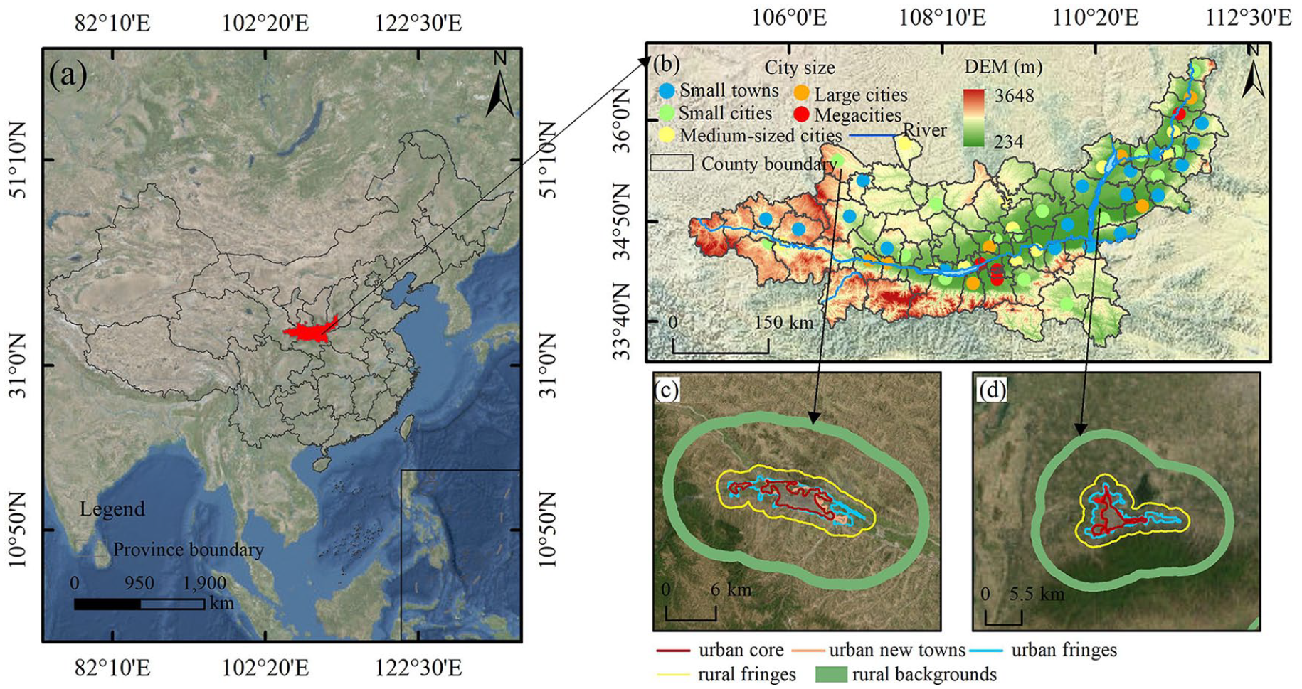
Location of the GPUA in China (a), geographical distribution and city sizes of 55 cities in the GPUA (b), urban core, urban new towns, urban fringes, rural fringes, and rural backgrounds for three urban (UC, UNT and UF) subzones and two rural (RF and RB) subzones for Kongtong (c) and Yongji (d). UC, UNT, UF, RF and RB represent the urban core, urban new towns, urban fringes, rural fringes, and rural backgrounds, respectively.

Data sources and processing

Landsat time series

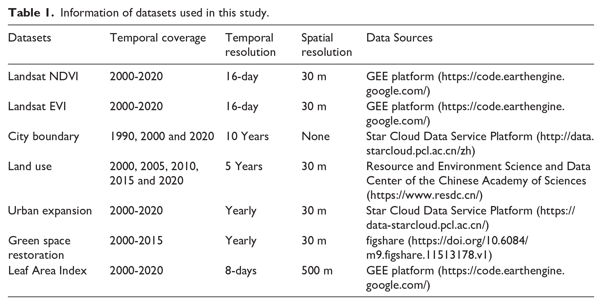
The Landsat 5, 7, and 8 surface reflectance (SR) data, covering the period 2000-2020, was obtained from the United States Geological Survey (USGS). With a temporal resolution of 16 d and a spatial resolution of 30 m, the data underwent atmospheric correction to eliminate errors caused by atmospheric scattering, absorption, and reflection (Table 1). Initially, this study used the "filter" function on the GEE platform (https://code.earthengine.google.com/) to refine the Landsat EVI dataset specifically for the GPUA (Figure 2). Subsequently, the QA (Quality Assessment) band of SR remote sensing images was employed to conduct a bitwise operation, effectively filtering out undesirable image elements such as clouds, cloud shadows, and snow to enhance clarity and remove obstruction. Using the maximum value synthesis method, the annual maximum EVI data and NDVI (Normalized Difference Vegetation Index) were calculated from 2000 to 2020 (Li et al., 2019). These refined datasets were then used to analyze the vegetation change trends with a spatial resolution of 30 m×30 m along the urban-rural gradient within the GPUA.

Table 1.

Information of datasets used in this study.

Datasets	Temporal coverage	Temporal resolution	Spatial resolution	Data Sources
Landsat NDVI	2000-2020	16-day	30 m	GEE platform (https://code.earthengine.google.com/)
Landsat EVI	2000-2020	16-day	30 m	GEE platform (https://code.earthengine.google.com/)
City boundary	1990, 2000 and 2020	10 Years	None	Star Cloud Data Service Platform (http://data.starcloud.pcl.ac.cn/zh)
Land use	2000, 2005, 2010, 2015 and 2020	5 Years	30 m	Resource and Environment Science and Data Center of the Chinese Academy of Sciences (https://www.resdc.cn/)
Urban expansion	2000-2020	Yearly	30 m	Star Cloud Data Service Platform (https://data-starcloud.pcl.ac.cn/)
Green space restoration	2000-2015	Yearly	30 m	figshare (https://doi.org/10.6084/m9.figshare.11513178.v1)
Leaf Area Index	2000-2020	8-days	500 m	GEE platform (https://code.earthengine.google.com/)

Figure 2.

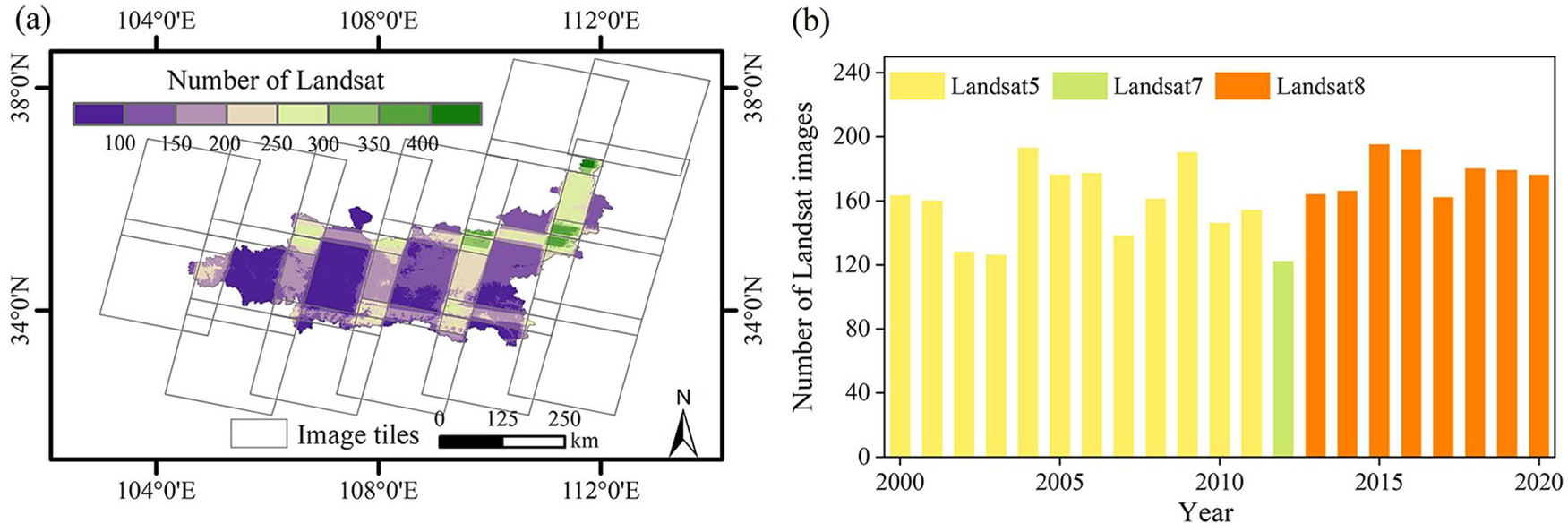
Availability of Landsat images. Spatial pattern (a) and time variation (b) of the number of images by sensors Landsat 5/7/8 in the GPUA from 2000 to 2020.

City boundaries data

The city boundary data for the years 1990, 2000 and 2020 were sourced from the Star Cloud Data Service Platform (http://data.starcloud.pcl.ac.cn/zh). This dataset was extracted from 30-m-resolution Landsat imagery using a globally consistent boundary definition and drawing method, ensuring precise capture of the contour features of urban and rural marginal areas (Chen et al., 2022a; Li et al., 2020b; Zhang et al., 2022). This dataset has become widely used for distinguishing urban and rural zones (Li et al., 2023; Zhang et al., 2022).

Land use and urban expansion data

Land use data for the years 2000, 2005, 2010, 2015 and 2020 were acquired from the Resource and Environment Science and Data Center of the Chinese Academy of Sciences (https://www.resdc.cn/). This dataset was generated by interpreting Landsat TM/ETM/OLI image data through human-computer interaction, offering a spatial resolution of 30 m × 30 m and an accuracy exceeding 90% (Ning et al., 2018). To mitigate the influence of water bodies on vegetation change trends, water body pixels were masked out. In addition, annual urban expansion data for the GPUA spanning from 2000 to 2020 were sourced from the Star Cloud Data Service Platform (https://data-starcloud.pcl.ac.cn/). This dataset, created on the GEE platform, was applied to evaluate the impact of urban expansion on vegetation trends across the urban-rural gradient in the GPUA.

Other data

The green space restoration dataset was acquired from figshare (https://doi.org/10.6084/m9.figshare.11513178.v1). This dataset offers a high resolution of 30 meters and covers the period from 2000 to 2015, with an overall accuracy exceeding 80% (Liu et al., 2020). This dataset was used to quantitatively evaluate the impact of green space restoration on EVI change trends (Liu et al., 2020). Because the available data was only updated until 2015, the 2015 data was used as a substitute for 2020. Additionally, the Leaf Area Index (LAI) data, with spatial and temporal resolutions of 500 meters and 8 days spanning from 2000 to 2020, was derived from the MOD15A2H data product on the GEE platform (Table 1). A yearly temporal interval of LAI was calculated by maximum value composite (MVC) method. This dataset was mainly applied to assess the efficacy of Landsat EVI in estimating vegetation change trends. Figure 3 indicates the framework for identification and attribution of EVI change trends across the urban-rural gradient.

Figure 3.

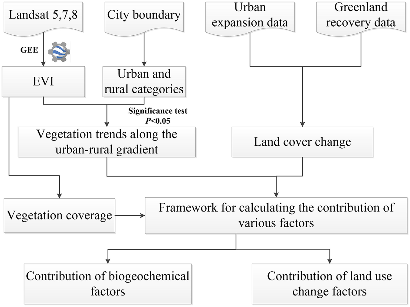
The framework for identification and attribution of EVI change trends across the urban-rural gradient.

Methods

Definition of urban boundaries and size

In this study, three urban subzones, namely urban cores (UC), urban new towns (UNT), and urban fringes (UF), as well as two rural subzones, namely rural fringes (RF) and rural backgrounds (RB) were defined based on city boundaries in 1990, 2000 and 2020 (Li et al., 2023). Specifically, UC, UNT, and UF represent urban boundaries in 1990, the period between 1990 and 2000, and the period between 2000 and 2020, respectively (Figure 1c and d). RF is defined as a buffer area around the urban zone with a distance of d, ensuring its total area matches the combined areas of the three urban subzones. For the calculation method of d refer to Zhang et al. (2022). Conversely, RB is defined as a buffer zone far from the city, with its area equivalent to the combined area of the urban subzones. The distance from the UF area to RB was set at 5d to minimize the influence of urbanization (Figure 1c and d) (Du et al., 2019; Li et al., 2023).

The study selected 55 county-level cities within the GUPA, excluding urban areas less than 5.0 km² in 2020. According to Li et al. (2023), the urban area of the GPUA in 2020 was divided into five categories based on the “pyramid” shape (Figure 1b), These categories include 18 small towns (32.7% of the total, with urban areas less than 25 km²), 15 small cities (27.3%, with urban areas ranging from 25km² to 50 km²), 11 medium-sized cities (20.0%, with urban areas ranging from 50 km² to 110km²), seven large cities (12.7%, with urban areas ranging from 110km² to 180km²) and four megacities (7.3%, with urban areas greater than 180 km²).

Analysis of EVI trends across the urban-rural gradient

The vegetation change trend in the GPUA from 2000 to 2020 was calculated using the Theil-Sen median trend analysis, a robust non-parametric method that is sensitive to data distribution and outliers, ensuring reliable results which were calculated using Eq. (1) (Sen, 1968).

β = m e d i a n (\frac{E V I_{i} - E V I_{j}}{i - j}, \forall_{i} < j)

(1)

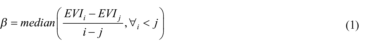
where i and j denote the time series numbers, while EVI_i and EVI_j represent the maximum EVI values in years i and j, respectively. A positive value of β indicates increasing EVI, while a negative value indicates decreasing EVI. The significance of the trend was evaluated using the Mann-Kendall method, a non-parametric statistical test that can effectively reduce the impact of data outliers (Jiang et al., 2015; Kendall, 1975; Masroor et al., 2020). Only statistically significant changes in EVI trends at a significance level of 0.05 were considered when investigating vegetation changes along the urban-rural gradient. Simultaneously, water body pixels were excluded based on land cover data.

Analysis of EVI change drivers

The determinants factors of EVI variation trends can be systematically categorized into two principal domains: biogeochemical driving factors and land cover changes (Chen et al., 2019; Li et al., 2023; Piao et al., 2020; Zhu et al., 2016). The biogeochemical component encompasses atmospheric CO2 dynamics, nitrogen deposition patterns, and climatic change, while land cover changes primarily manifest through urban expansion processes and urban greening initiatives. Due to the inherent complexity in disentangling the individual contributions of atmospheric CO₂ fertilization, nitrogen deposition, and climate change impacts on urban vegetation dynamics at municipal scales (Zhao et al., 2016), these factors are collectively conceptualized as integrated biogeochemical drivers (Li et al., 2023). The effect of biogeochemical drivers on vegetation is categorized into the background biogeochemical drivers (BBD) and urban biogeochemical drivers (UBD). BBD encompasses large-scale environmental changes, such as rising atmospheric CO₂ concentration, nitrogen deposition, and global warming (Li et al., 2023; Piao et al., 2020; Zhu et al., 2016). On the other hand, UBD includes local (city) scale environmental changes, such as urban CO₂ emissions and urban heat island effect, and air pollution (Roxon et al., 2020; Zhao et al., 2016).

Land use changes can impact vegetation through two main mechanisms: urban expansion or densification (UED) and urban green recovery (UGR). UED refers to the effects of urban expansion, such as the conversion of grassland, woodland, or farmland into impermeable surfaces, which typically lead to a decrease in vegetation activity intensity (Li et al., 2022; Zhuang et al., 2023). Conversely, UGR involves the construction of urban green spaces, which usually increase vegetation activity intensity (Bille et al., 2023; Shahtahmassebi et al., 2021). In addition, a residual factor (REF) is used to account for the influence of other factors, such as estimation errors, changing in building height, the frequency of heat waves, and disturbances caused by pests on the vegetation change trends (Nighswander et al., 2021; Zhang et al., 2015; Zou et al., 2021). Therefore, the observed EVI trends in this study can be expressed by the following equation:

O B S_{E V I} = B B D_{E V I} + U B D_{E V I} + U E D_{E V I} + U G R_{E V I} + R E F_{E V I}

(2)

where, the OBS_EVI represents the actual observed EVI; the UBD_EVI, BBD_EVI, UED_EVI, UGR_EVI, and REF_EVI signify the impacts of UBD, BBD, UED, UGR, and other factors influencing the EVI, respectively.

To further analyze the impacts of UBD, BBD, UED, and UGR on vegetation across the urban-rural gradient, urban expansion pixels (Pix-ED), green space restoration pixels (Pix-GR), the stable land cover with a rising EVI trend (Pix-PE) and stable land cover with a decreasing EVI trend (Pix-NE) were categorized based on land use and EVI changes characteristics. In the GPUA, Pix-ED, Pix-GR and Pix-PE collectively represented 96.9% of the pixels, while Pix-NE accounted for only 3.1%. The contributions of BBD and UBD to the vegetation change trends can be expressed by the following equations (Li et al., 2023).

B B D_{E V I} = B B D_{P i x_{-} P E} + B B D_{P i x_{-} E D} + B B D_{P i x_{-} G R}

(3)

U B D_{E V I} = U B D_{P i x_{-} P E} + U B D_{P i x_{-} E D} + U B D_{P i x_{-} G R}

(4)

where BBD_{Pix_PE}, BBD_{Pix_ED}, BBD_{Pix_GR}, UBD_{Pix_PE}, UBD_{Pix_ED} and UBD_{Pix_GR} represent the impacts of BBD and UBD on EVI for Pix-PE, Pix-ED and Pix-GR, respectively. Pix-NE was excluded due to its small portion (<4%) and its susceptibility to other factors such as changes in building heights, diseases, and insect pests.

UED and UGR exclusively impact the vegetation change trends of Pix_ED with urban expansion and Pix_GR with green recovery, respectively. Therefore, the contributions of UED and UGR to EVI trends can be represented by the following equation:

U E D_{EVI} = U E D_{Pix_ED}

(5)

U G R_{EVI} = U G R_{Pix_GR}

(6)

where UED_{Pix_ED} and UGR_{Pix_GR} indicate the influence of UED and UGR on the EVI trends in Pix-ED and Pix-GR, respectively.

Based on the Eqs. (3) to (6), the calculation of the contribution ratio of BBD_EVI, UBD_EVI, UED_EVI, and UGR_EVI can be converted to estimate the BBD_{Pix_PE}, BBD_{Pix_ED}, BBD_{Pix_GR}, UBD_{Pix_PE}, UBD_{Pix_ED}, UBD_{Pix_GR}, UED_{Pix_ED}, and UGR_{Pix_GR}. BBD_{Pix_PE} was quantified as the contribution of BBD to rural background EVI, determined by the ratio of urban-rural background vegetation coverage and the number of pixels with stable land cover and a rising EVI trend in relation to the total number of pixels. UBD_{Pix_PE} represents the impact of UBD on the Pix_PE’s EVI change trend in the UC, UNT or UF. BBD_{Pix_ED} is defined as the influence of BBD on the Pix_ED’s EVI trend in the UC, UNT, or UF, while UBD_{Pix_ED} is the contribution of UBD to Pix_ED’s EVI trend in the UC, UNT, or UF.

BBD_{Pix_PE} was quantified as the contribution of BBD to rural background EVI, determined by the ratio of urban-rural background vegetation coverage and the number of pixels with stable land cover and a rising EVI trend in relation to the total number of pixels. This can be expressed by the following equation:

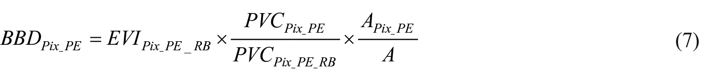
B B D_{P i x_{-} P E} = E V I_{P i x_{-} P E_R B} \times \frac{P V C_{P i x_{-} P E}}{P V C_{P i x_{-} P E_{-} R B}} \times \frac{A_{P i x_{-} P E}}{A}

(7)

where EVI_{Pix_PE_RB} denotes the average EVI change trend for the Pix_PE type in RB. The percent vegetation cover (PVC) was derived from 30m NDVI data using the pixel dichotomy method (Gao et al., 2020). PVC_{Pix_PE} and PVC_{Pix_PE_RB} denote the PVC values of Pix_PE for UC, UNT, UF, and RB, respectively. A and A_{Pix_PE} indicate the total number of pixels and Pix_PE for a specific city subzone (UC, UNT or UF), respectively.

UBD_{Pix_PE} represents the impact of UBD on the Pix_PE’s EVI change trend in the UC, UNT or UF. It can be expressed by the following equation:

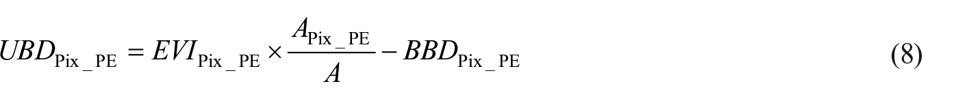
U B D_{Pix_PE} = E V I_{Pix_PE} \times \frac{A_{Pix_PE}}{A} - B B D_{Pix_PE}

(8)

where EVI_{Pix_PE} denotes the average EVI change trend for Pix_PE in the UC, UNT, or UF. BBD_{Pix_ED} is defined as the influence of BBD on the Pix_ED’s EVI trend in the UC, UNT, or UF, while UBD_{Pix_ED} is the contribution of UBD to Pix_ED’s EVI trend in the UC, UNT, or UF. They can be calculated using the following equations:

B B D_{P i x_{-} E D} = E V I_{P i x_{-} U L C} \times \frac{B B D_{P i x_{-} P E}}{B B D_{P i x_{-} P E} + U B D_{P i x_{-} P E}} \times \frac{A_{P i x_{-} E D}}{A}

(9)

U B D_{P i x_{-} E D} = E V I_{P i x_{-} U L C} \times (1 - \frac{B B D_{P i x_{-} P E}}{B B D_{P i x_{-} P E} + U B D_{P i x_{-} P E}}) \times \frac{A_{P i x_{-} E D}}{A}

(10)

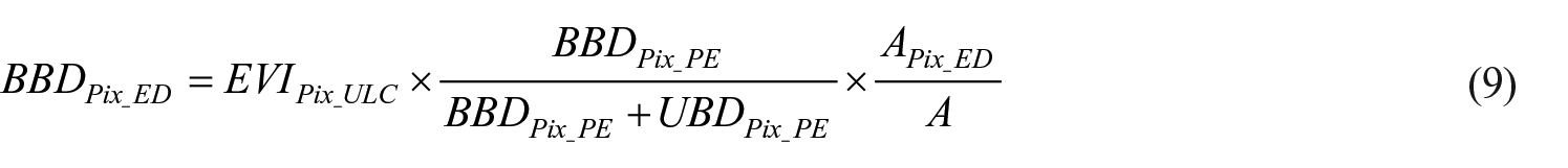
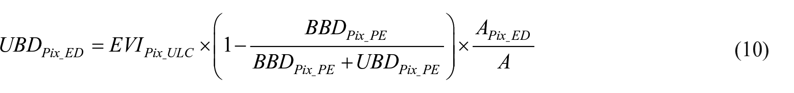
where EVI_{Pix_ULC} denotes the average EVI change trend of Pix_ULC in the UC, UNT, or UF. A and A_{Pix_PE} denote the total number of pixels and Pix_ED for a specific city subzone (UC, UNT, or UF), respectively.

UED_{Pix_ED} signifies the influence of UED on Pix_ED’s EVI change trend in the UC, UNT or UF. It can be expressed by the following equation:

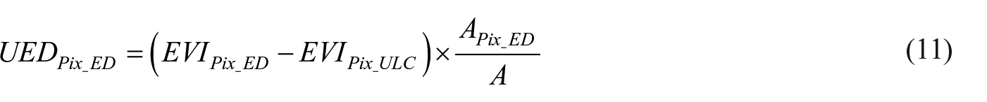
U E D_{P i x_{-} E D} = (E V I_{P i x_{-} E D} - E V I_{P i x_{-} U L C}) \times \frac{A_{P i x_{-} E D}}{A}

(11)

where EVI_{Pix_ED} denotes the average EVI change trend of Pix_ED in the UC, UNT, or UF.

UGR_{Pix_GR} indicates the influence of UGR on Pix_GR’s EVI trend in the UC, UNT, or UF, with an estimation method similar to that of UED_{Pix_ED}.

Percentage contribution of each driver

In order to facilitate a more comprehensive comparison of each driving factor’s contribution, the contribution percentage of each driving factor were calculated using the following equation:

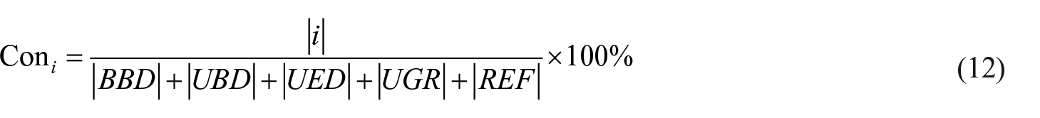
{Con}_{i} = \frac{| i |}{| B B D | + | U B D | + | U E D | + | U G R | + | R E F |} \times 100 %

(12)

where Con_i indicates the percentage contribution of the drivers to observed change trend in EVI (i = BBD, UBD, UED, UGR, and REF).

Results

EVI change trends across the urban-rural gradient in the GPUA

The EVI change trends across 55 cities of the GPUA from 2000 to 2020 are depicted in Figure 3 for the UC, UNT, UF, RF, and RB. In the UC, the EVI change trend was 0.0459 ± 0.0080/10a, with 83.64% of cities exhibiting an increasing trend. Conversely, only 16.36% of cities showed a decreasing trend in EVI, mainly concentrated in the central GPUA (Figure 4a and f). For the UNT, the EVI change trend was 0.0347 ± 0.0093/10a, with 58.18% and 41.82% of cities showing increasing and decreasing trends, respectively. Cities with an increasing trend were mainly located in the middle and eastern GPUA (Figure 4b and f). In the UF, the EVI change trend turned negative (-0.0090 ± 0.0121/10a), with 30.91% and 69.09% of cities exhibiting increasing and decreasing trends, respectively. Cities with a decreasing trend were mainly situated in the middle and western GPUA (Figure 4c and f). The average EVI change trend in RF and RB became positive again (0.0738 ± 0.0075/10a and 0.0817 ± 0.0082/10a), with 85.45% and 98.18% of cities showing an increasing trend (Figure 4d and f). Overall, a V-shaped pattern of EVI change trends was observed from UC to RB (Figure 4f).

Figure 4.

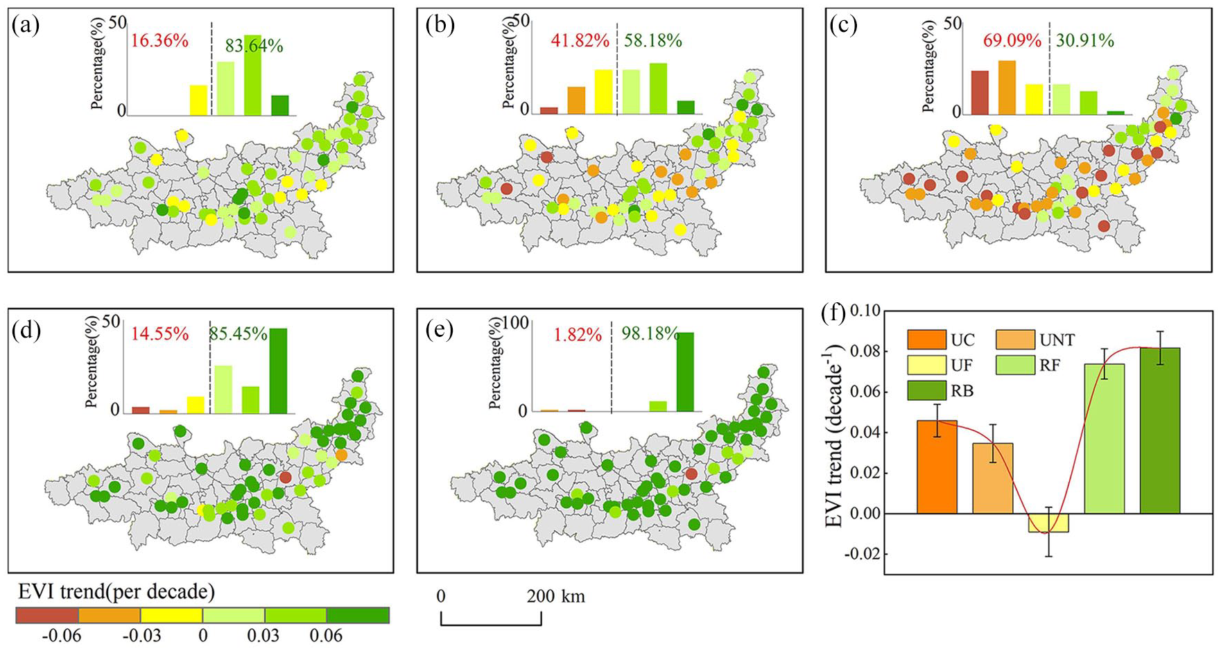
The EVI change trends in UC, UNT, UF, RF and RB for 55 cities in GPUA. Mean EVI change trends for UC (a), UNT (b), UF (c), RFs (d), RB (e), and comparisons among urban and rural subzones (f).

Urban-rural gradient of the EVI change trend across city sizes

The EVI change trends across city sizes were evaluated for the three urban (UC, UNT, and UF) and two rural subzones (RF and RB) (Figure 5). Generally, there was a gradual increase in EVI change trends from small towns to megacities for the three urban subzones (UC, UNT, and UF) (Figure 5). Specifically, the EVI change trend for UC increased from 0.0333 ± 0.0058/10a to 0.0520 ± 0.0091/10a with increasing city size. Similarly, in the UNT and UF, the EVI change trends increased from 0.0281 ± 0.0077/10a and -0.0189 ± 0.0082/10a in small towns to 0.0402 ± 0.0120/10a and -0.0114 ± 0.0042/10a in megacities, indicating a gradual upward trend with city size expansion (Figure 5). The EVI change trends for the two rural subzones (RF and RB) remained stable across city sizes. In the RF, medium-sized cities exhibited the highest EVI change rate, at 0.0729 ± 0.0068/10a, while large cities had the lowest at 0.0661 ± 0.0067/10a. Conversely, in the RB, large cities experienced the highest change at 0.0864 ± 0.0105/10a, while megacities had the lowest at 0.0795±0.0092/10a (Figure 5).

Figure 5.

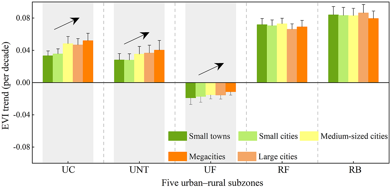
EVI change trends of three urban (UC, UNT, and UF) and two rural subzones (RF and RB) in the GPUA across city size.

Influencing factors of EVI change trend across urban-rural gradient

Biogeochemical drivers exert a more significant influence on EVI change trends compared to land use changes for the UC and UNT (Figure 6a and b). In the UC, biogeochemical drivers and land use changes accounted for 79.2% and -15.2% of the EVI change trend in the GPUA, with contribution from UBD, BBD, UED, and UGR at 51.9% (0.0416 ± 0.0049 per decade), 27.3% (0.0219 ± 0.0030 per decade), -16.7% (-0.0134 ± 0.0022 per decade), and 1.50% (0.0012 ± 0.0017 per decade), respectively (Figure 6a and f). Similarly, in the UNT, biogeochemical drivers and land use changes contributed 67.9% and -28.79% to the EVI change trend, with contributions from UBD, BBD, UED, and UGR at 37.2% (0.0319 ± 0.0083 per decade), 30.7% (0.0263 ± 0.0055 per decade), -29.6% (-0.0253 ± 0.0076 per decade), and 0.8% (0.0007 ± 0.0033 per decade), respectively (Figure 6b and f). Conversely, in the UF, land use changes predominantly regulated EVI change trends (-51.4%), with biogeochemical drivers contributing 45.0%. Here, UED played a key role in driving EVI change trends, with contributions from UBD, BBD, UED, and UGR at 15.8% (0.0148 ± 0.0051 per decade), 29.2% (0.0254 ± 0.0051 per decade), -51.9% (-0.0504 ± 0.0069 per decade), and 0.6% (0.0005 ± 0.0023 per decade), respectively (Figure 6c and f). In the rural subzones, biogeochemical drivers predominantly determined EVI change trends, contributing 85.5% and 94.0% for RF and RB, respectively, while land cover changes play a minor role at -12.3% and -3.8%, respectively. Specifically, in the RF, contributions from UBD, BBD, UED, and UGR were 15.3% (0.0144 ± 0.0027 per decade), 70.2% (0.0663 ± 0.0045 per decade), -12.5% (-0.0118 ± 0.0022 per decade) and 0.2% (0.0002 ± 0.0013 per decade), respectively. In RB, contributions from BBD and UED were 94.01% (0.0846 ± 0.0076 per decade) and -3.8% (-0.0034 ± 0.0026 per decade) (Figure 6d, 4e, and 6f). Overall, the contribution of UBD decreased gradually along the urban-rural gradient, from 51.9% in the UC to 0% in the RB, with the highest value (51.9%) observed in the UC.

Figure 6.

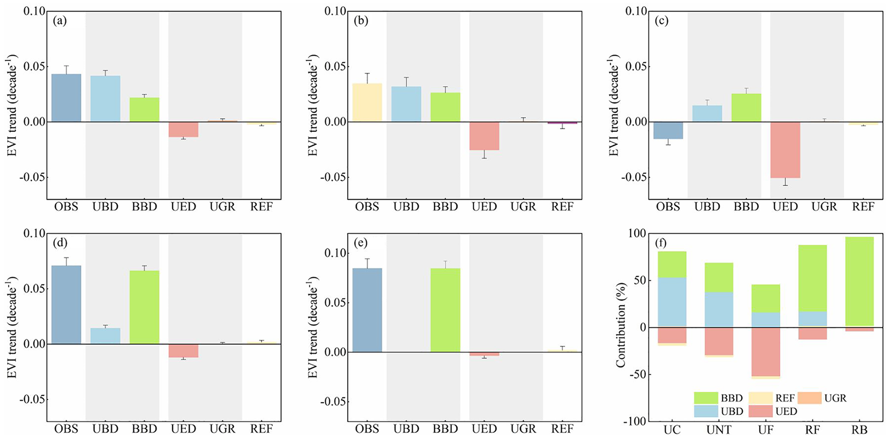
Contributions of biogeochemical driving factors and land use changes to EVI change trends for the UC (a), UNT (b), UF (c), RF (d), RB (e), and comparisons among urban and rural subzones (f).

Influencing factors of EVI change trend across city sizes

The contributions of each driving factor along the urban-rural gradient were also analyzed across different city sizes (Figure 7). The EVI change trends showed a gradual increase with the increase of city size for the three urban subzones (UC, UNT, and UF). Specifically, the contribution of UBD in UC exhibited an increase from 0.0327 ± 0.0047 per decade in small towns to 0.0412 ± 0.0053 per decade in megacities (Figure 7a). Similarly, in the UNT, the UBD contribution increased by 0.0246 ± 0.0042 per decade in small towns to 0.0381 ± 0.0069 per decade in megacities (Figure 7b). Likewise, in the UF, the UBD contribution rose from 0.0096 ± 0.0026 per decade in small towns to 0.0221 ± 0.0076 per decade in megacities (Figure 7c). Additionally, the contribution of UED to the EVI change trend also exhibited a gradual increase with the increase of city size. The negative impact of UED in the UNT increased from -0.0226 ± 0.0044 per decade in small towns to -0.0269 ± 0.0047 per decade in megacities (Figure 7b). Similarly, in the UF, the negative effect of UED rose from -0.0483 ± 0.0062 per decade in small cities to -0.0559 ± 0.0083 per decade in megacities (Figure 7c). In the UC, UED demonstrated the least contribution (-0.0099 ± 0.0034 per decade) in megacities and the most negative contribution (-0.0499 ± 0.0064 per decade) in small towns (Figure 7a). However, there were no noticeable variations in driving factors with the increase in city size in the two rural subzones (RF and RB) (Figure 7d and e).

Figure 7.

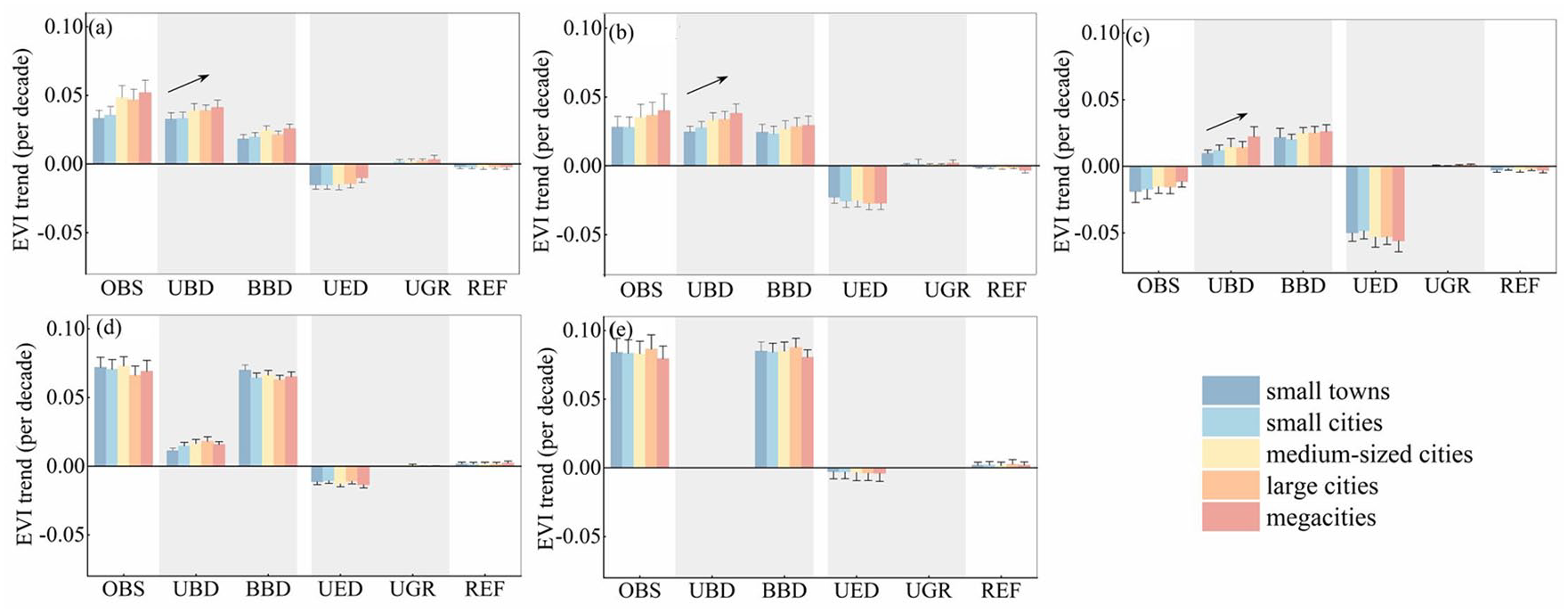
The contribution of each factor to the EVI change trends across different city sizes for the UC (a), UNT (b), UF (c), RF (d) and RB (e).

Discussion

EVI change trends in the urban and rural subzones

Urban agglomerations serve as the core regions for China's socio-economic development. (Fang and Yu, 2020; Wang et al., 2022). Given the rapid urbanization, it is imperative to explore the dynamics of vegetation and its response to changes in land use and biogeochemical factors across the urban-rural gradient (Jia et al., 2021). Previous studies have highlighted the significance of small cities or towns in shaping the quality of future urbanization, emphasizing the importance of monitoring vegetation dynamics in these areas (Fahmi et al., 2014; Li et al., 2023). In this study, high-resolution remote sensing data (30 m × 30 m) from Landsat EVI was used to characterize vegetation change trends along the urban-rural gradient. The results revealed that the EVI change trend in UC surpassed that of other urban subzones (UNT and UF) from 2000 to 2020 (Figure 4f). Li et al. (2023) analyzed the vegetation change trends along the urban-rural gradient in 1500-plus cities of China by the MODIS NDVI and EVI (250 m), and indicated that vegetation change trends also exhibited a V-shaped pattern along with the urban-rural gradient. Timely and rapid monitoring of urban vegetation using remote sensing data with coarse spatial resolution and high temporal resolution is crucial for understanding the characteristics of urban greening at large scale (Zhang et al., 2024). However, these results are of limited use from the perspective of urban green space planning and management (Zhang et al., 2024). Landsat EVI with a high spatial resolution can better analyze the vegetation change trends along with the urban-rural gradient at the level of small lawns, residential parks or other small areas of residential greenery (Zhang et al., 2024; Zhao et al., 2023). These results are directly used in urban green space planning and ecosystem services management of cities. The observed V-shaped trend of EVI from UC to RB can be attributed to a combination of the decline of surrounding vegetation caused by urbanization (Li et al., 2020a; Zhong et al., 2021) and increasing green vegetation driven by biogeochemical factors (Piao et al., 2020; Shen et al., 2022). From the urban cores to the urban fringes, the trend in EVI progressively declines, with the UC and UNT exhibiting an increasing trend (Figure 4f). This suggests that the factors such as rising CO₂ concentration, nitrogen deposition, and temperature increase in the inner urban environment promote the growth of vegetation (Deng et al., 2020; Langley and Megonigal, 2010; Yang et al., 2023). In contrast, the EVI in the urban fringes shows a downward trend (Figure 4f), primarily due to urban expansion, which converts cultivated land, grassland or forests into impervious surfaces, thereby reducing the vegetation cover (Dou and Han, 2021; Guan et al., 2023, Zhao et al., 2023). From the urban fringes to the rural backgrounds, the EVI trend gradually reverses, shifting from a decline to an increase (Figure 4f). This is attributed to the fact that rural areas are less affected by urbanization, and climate change or ecological engineering construction can also promote the growth of vegetation. Furthermore, EVI change trends in UC, UNT, and UF exhibited an overall increase with the increase of city size, indicative of the heightened emphasis on urban greening in cities with a more developed economy and larger scale. Conversely, no discernible changes in EVI trends were noted with increasing city size in the two rural areas (Figure 7). This phenomenon is attributed to the intensification of human activities in larger cities, resulting in increased CO₂ concentrations and surface temperatures that further stimulate the growth of vegetation (He et al., 2022; Reddy et al., 2010; Zhang et al., 2022).

Analysis of factors affecting EVI change trend

The influence factors analysis reveals that the increase in EVI in UC is primarily driven by UBD (Figure 6), consistent with previous studies highlighting the prevalent phenomenon of vegetation enhancement in urban areas, primarily attributed to urban biogeochemical factors (Dobbs et al., 2017; Tang et al., 2021). Conversely, the decrease in EVI in UF is mainly affected by UED, likely due to the conversion of grasslands, forestland, and croplands into impervious surfaces (Li et al., 2023; Zhang et al., 2022). These findings underscore the contrasting trends in urban vegetation, characterized by a positive trend under the dominance of biogeochemical factors and a negative trend under the dominance of land use changes (such as urban sprawl) (Xie et al., 2020). Our results exhibit a distinct contrast to the patterns observed in natural ecosystems, where biogeochemical drivers and land-cover change (e.g., afforestation) consistently demonstrate synergistic effects in promoting vegetation greening (Chen et al., 2019; Zhu et al., 2016). For cities of varying sizes, the contribution of UBD increases with city size across all three types of urban areas (Figure 7). This can be attributed to the faster development of the larger cities, which place greater emphasis on urban greening initiatives (Zhang et al., 2022). Additionally, human activities in the larger cities are more intense, resulting in elevated CO₂ concentration, surface temperature and nitrogen deposition rates. These factors, in turn, promote vegetation growth (Peng et al., 2024). The impact of UED is more pronounced in UNT and UF of larger cities and megacities (Figure 7). In contrast, the effect is relatively weaker in UC, likely due to the more significant urban expansion and densification observed in UNT and UF of larger cities and megacities, intensifying the influence of urban expansion dynamics on vegetation (Alam and Banerjee, 2023). Compared with the study by Li et al. (2023), this study utilizes higher-resolution 30 m spatial images to examine at the urban agglomeration scale. The conclusions drawn are consistent with those of Li et al. (2023), further validating the accuracy of the results regarding vegetation change trends along the urban-rural gradient and the contribution of each driving factor at the urban agglomeration scale.

Validation of other results from other vegetation indices and urban/rural definitions

Previous studies have highlighted the sensitivity of NDVI to variation in sparse vegetation cover, making it a valuable tool for detecting urban vegetation dynamics (Zhang et al., 2024). Therefore, NDVI and LAI were used to verify the influence of different satellite data sources on EVI measurements in the GPUA. The results showed consistency among the three data sources (Figure 8), with correlation coefficients of 0.92 for NDVI-EVI and 0.83 for LAI-EVI, indicating minimal influence of satellite data on the study results (Figure 8). EVI, known for its ability to reduce the atmospheric and soil background values, has been widely used in monitoring urban and surrounding vegetation (Zhou et al., 2014). Notably, the definition of urban/rural areas also affected EVI change trends along the urban-rural gradient (Li et al., 2023). To enhance the analysis, seven urban subzones (Urban 1-7 were divided using city boundary data from before 1990, from 1990 to 1995, from 1995 to 2000, from 2000 to 2005, from 2005 to 2010, from 2010 to 2015, and from 2015 to 2020) and five rural subzones (Rural 1-5 were buffers around the UF with distances of 1d to 5d) were further defined in this study. The results exhibited similarities to those obtained using the five urban-rural subzones classifications (Figure 9), indicating that the five urban-rural classification systems better represent EVI change along the urban-rural gradient in the GPUA. This approach provides a more detailed reflection of EVI variability across the urban-rural gradient compared to previous studies that only divided areas into old and new urban areas or simply extracted urban and rural areas for analysis (Zhao et al., 2023).

Figure 8.

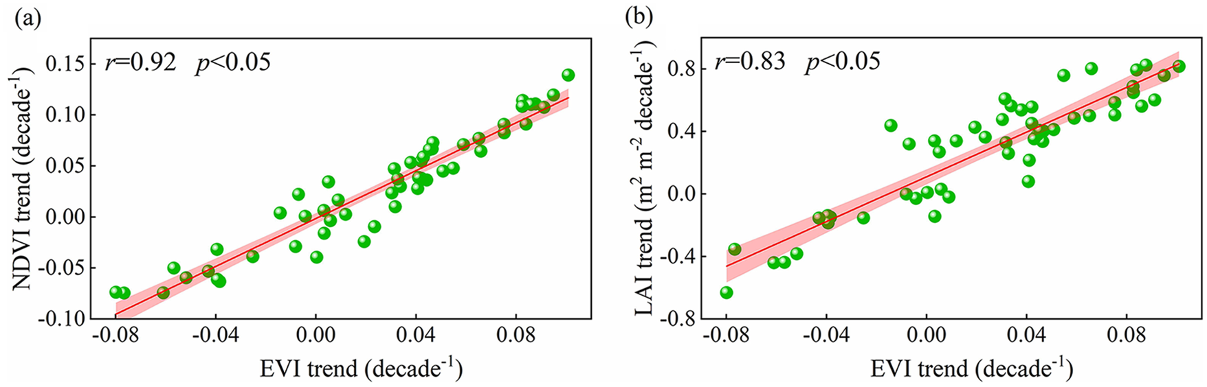
Comparison of EVI trend and NDVI trend (a) and EVI trend and LAI trend (b) of 55 cities in the GPUA.

Figure 9.

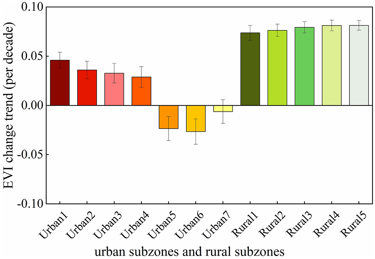
EVI urban-rural gradient trend of GPUA based on 12 urban-rural categories.

Uncertainties and future studies

This study has several limitations worth noting. Firstly, the CO₂ fertilization effects can vary across different vegetation types or tree ages. Due to the lack of data on detailed vegetation type and tree age in these cities, variations in the background biogeochemical effects on vegetation between urban and rural regions could not be adequately accounted for. Secondly, the analysis focused on annual maximum EVI, typically occurring in July or August, potentially overlooking seasonal variations in vegetation change trends. Additionally, while efforts were made to improve data quality by pre-processing in the GEE platform to eliminate noise such as cloud shadows and aerosol particles, the effectiveness of this process may not be exhaustive. (Jin et al., 2024). Lastly, other factors such as building height, pests, and plant diseases may also affect vegetation change trends. Moving forward, it is essential to employ more precise data and robust methodologies to comprehensively assess vegetation dynamics and their responses to land use changes and biogeochemical factors across the urban-rural gradient in urban agglomeration areas.

Conclusions

This study explored vegetation change trends along the urban-rural gradient for 55 cities in the GPUA using Landsat EVI data from 2000 to 2020. Additionally, we analyzed the contributions of biogeochemical drivers (BBD and UDB) and land use changes (UED and UGR) to these trends. Our results showed a pattern of increasing EVI in the UC and UNT, followed by a decrease in the UF, and subsequent increase in the RF and RB, forming a V-shaped trend along the urban-rural gradient. Biogeochemical drivers exert a more significant influence on EVI change trends compared to land use changes for the UC and UNT. Conversely, land use changes predominantly regulated EVI change trends in the UF. In the RF and RB, biogeochemical drivers predominantly determined EVI change trends. This study explored the vegetation changes and their responses to land use changes and biogeochemical factors across the GPUA, offering valuable insights into understanding vegetation dynamics across the urban-rural gradients in urban agglomerations.

Footnotes

Author contributions

All authors contributed to the study’s conception and design. Conceptualization, methodology, formal analysis, and data curation were performed by Anzhou Zhao and Zihan Jin. Sample analysis, software, visualization, and investigation were performed by Lili Feng. The first draft of the manuscript was written by Anzhou Zhao and Zihan Jin. All authors commented on previous versions of the manuscript. All authors read and approved the final manuscript.

Declaration of conflicting interests

The author(s) declared no potential conflicts of interest with respect to the research, authorship, and/or publication of this article.

Funding

The author(s) disclosed receipt of the following financial support for the research, authorship, and/or publication of this article: This research was supported by the National Natural Science Foundation of China (42171212, 42301178) and the National Natural Science Foundation of Hebei Province of China (D2022402030)

ORCID iD

Anzhou Zhao

Data availability statement

The data that support the findings of this study are available from the corresponding author upon reasonable request.

Author biographies

Anzhou Zhao is a Professor at the School of Mining and Surveying Engineering, Hebei University of Engineering. And he received the PhD degree from Beijing Normal University of China. His research areas include remote sensing applications in the ecological environment and agriculture.

Zihan Jin is a master ‘s student in the School of Mining and Surveying Engineering at Hebei University of Engineering. His research area is the impact of urban expansion on vegetation.

Lili Feng is an assistant researcher at the Chinese Academy of Forestry. Her research area is the remote sensing monitoring of land degradation.

References

Alam

Banerjee

(2023) Characterizing land transformation and densification using urban sprawl metrics in the South Bengal region of India. Sustainable Cities and Society 89: 104295.

Anderson

Gough

(2020) Evaluating the potential of nature-based solutions to reduce ozone, nitrogen dioxide, and carbon dioxide through a multi-type green infrastructure study in Ontario, Canada. City and Environment Interactions 6: 100043.

Bille

Jensen

Buitenwerf

(2023) Global patterns in urban green space are strongly linked to human development and population density. Urban Forestry & Urban Greening 86: 127980.

Chen

Song

, et al. (2022a) Contrasting inequality in human exposure to greenspace between cities of Global North and Global South. Nature Communications 13(1): 4636.

Chen

Park

Wang

, et al. (2019) China and India lead in greening of the world through land-use management. Nature Sustainability 2(2): 122–129.

Chen

Wang

Zou

(2022b) Construction of an ecological security pattern based on ecosystem sensitivity and the importance of ecological services: A case study of the Guanzhong Plain urban agglomeration, China. Ecological Indicators 136: 108688.

Chen

Wang

Cescatti

, et al. (2023) Climate-driven vegetation greening further reduces water availability in drylands. Global Change Biology 29(6): 1628–1647.

Deng

Huang

Kim

, et al. (2020). Soil GHG fluxes are altered by N deposition: New data indicate lower N stimulation of the N2O flux and greater stimulation of the calculated C pools. Global Change Biology 26(4): 2613–2629.

Dobbs

Nitschke

Kendal

(2017) Assessing the drivers shaping global patterns of urban vegetation landscape structure. Science of the Total Environment 592: 171–177.

10.

Dou

Han

(2021) Quantifying land use/land cover change and urban expansion in Dongguan, China, from 1987 to 2020. IEEE Journal of Selected Topics in Applied Earth Observations and Remote Sensing 15: 201–209.

11.

Fang

, et al. (2019) Effects of rapid urbanization on vegetation cover in the metropolises of China over the last four decades. Ecological Indicators 107: 105458.

12.

Fahmi

Hudalah

Rahayu

, et al. (2014) Extended urbanization in small and medium-sized cities: The case of Cirebon, Indonesia. Habitat International 42: 1–10.

13.

Fang

(2020) China’s Urban Agglomerations. Cham: Springer.

14.

Feng

Yang

Jia

, et al. (2024) Variability of urban green space and its driving factors in 328 cities in China. Science China Earth Sciences 54: 486–502.

15.

Gao

Wang

Johnson

, et al. (2020). Remote sensing algorithms for estimation of fractional vegetation cover using pure vegetation index values: A review. ISPRS Journal of Photogrammetry and Remote Sensing 159: 364–377.

16.

Guan

Huang

, et al. (2023) Can land use/land cover optimization improve the environmental flow guarantee in regulated basins? Journal of Hydrology 626: 130309.

17.

Halecki

Stachura

Fudała

, et al. (2023) Assessment and planning of green spaces in urban parks: A review. Sustainable Cities and Society 88: 104280.

18.

Rosa

Lobell

, et al. (2023) The weekly cycle of photosynthesis in Europe reveals the negative impact of particulate pollution on ecosystem productivity. Proceedings of the National Academy of Sciences of the United States of America 120(49): e2306507120.

19.

Piao

Huntingford

, et al. (2022) Amplified warming from physiological responses to carbon dioxide reduces the potential of vegetation for climate change mitigation. Communications Earth & Environment 3(1): 160.

20.

Zhan

, et al. (2023) Urban-rural gradient in vegetation phenology changes of over 1500 cities across China jointly regulated by urbanization and climate change. ISPRS Journal of Photogrammetry and Remote Sensing 205: 367–384.

21.

Jia

Zhao

Zhang

, et al. (2021) Urbanization imprint on land surface phenology: The urban–rural gradient analysis for Chinese cities. Global Change Biology 27(12): 2895–2904.

22.

Jiang

Yuan

Wang

, et al. (2015) Spatio-temporal analysis of vegetation variation in the Yellow River Basin. Ecological Indicators 51: 117–126.

23.

Jin

Wang

Zong

, et al. (2024) Spatial patterns and driving forces of urban vegetation greenness in China: A case study comprising 289 cities. Geography and Sustainability 5: 370–381.

24.

Kendall

(1975) Rank Correlation Methods, Public Program Analysis. London, UK: Griffin.

25.

Langley

Megonigal

(2010) Ecosystem response to elevated CO₂ levels limited by nitrogen-induced plant species shift. Nature 466(7302): 96–99.

26.

Lekberg

Arnillas

Borer

, et al. (2021) Nitrogen and phosphorus fertilization consistently favor pathogenic over mutualistic fungi in grassland soils. Nature Communications 12: 3484.

27.

Liang

, et al. (2020a) The impacts of urbanization and climate change on urban vegetation dynamics in China. Urban Forestry & Urban Greening 54: 126764.

28.

Fang

, et al. (2022) Global impacts of future urban expansion on terrestrial vertebrate diversity. Nature Communications 13(1): 1628.

29.

Renssen

Roche

(2019) Global vegetation distribution driving factors in two Dynamic Global Vegetation Models of contrasting complexities. Global and Planetary Change 180: 51–65.

30.

Zhan

, et al. (2023) Competition between biogeochemical drivers and land-cover changes determines urban greening or browning. Remote Sensing of Environment 287: 113481.

31.

Gong

Zhou

, et al. (2020b) Mapping global urban boundaries from the global artificial impervious area (GAIA) data. Environmental Research Letters 15: 094044.

32.

Liu

Huang

, et al. (2020) High-spatiotemporal-resolution mapping of global urban change from 1985 to 2015. Nature Sustainability 3: 564–570.

33.

Masroor

Rehman

Avtar

, et al. (2020) Exploring climate variability and its impact on drought occurrence: Evidence from Godavari Middle sub-basin, India. Weather and Climate Extremes 30: 100277.

34.

Zhu

, et al. (2023) Impact assessment of urbanization on vegetation net primary productivity: A case study of the core development area in central plains urban agglomeration, China. Environmental Research 229: 115995.

35.

Nighswander

Sinclair

Dale

, et al. (2021) Importance of plant diversity and structure for urban garden pest resistance. Landscape and Urban Planning 215: 104211.

36.

Ning

Liu

Kuang

, et al. (2018) Spatio-temporal patterns and characteristics of land-use change in China during 2010–2015. Journal of Geographical Sciences 73: 789–802.

37.

Peng

Huang

Zhang

, et al. (2024) Exploring the impacts of urbanization on vegetation growth from the perspective of urban expansion patterns and maturity: A case study on 40 large cities in China. Sustainable Cities and Society 115: 105841.

38.

Peng

Zhang

, et al. (2022) Spatial expansion effects on urban ecosystem services supply-demand mismatching in Guanzhong Plain Urban Agglomeration of China. Journal of Geographical Sciences 32(5): 806–828.

39.

Piao

Wang

Park

, et al. (2020) Characteristics, drivers and feedbacks of global greening. Nature Reviews Earth & Environment 1(1): 14–27.

40.

Reddy

Rasineni

Raghavendra

(2010) The impact of global elevated CO₂ concentration on photosynthesis and plant productivity. Current Science 99: 46–57.

41.

Roxon

Ulm

Pellenq

RJM

(2020) Urban heat island impact on state residential energy cost and CO₂ emissions in the United States. Urban Climate 31: 100546.

42.

Schwaab

Meier

Mussetti

, et al. (2021) The role of urban trees in reducing land surface temperatures in European cities. Nature Communications 12(1): 6763.

43.

Sen

(1968) Estimates of the regression coefficient based on Kendall’s Tau. Journal of the American Statistical Association 63: 1379–1389.

44.

Seto

Guneralp

Hutyra

(2012) Global forecasts of urban expansion to 2030 and direct impacts on biodiversity and carbon pools. Proceedings of the National Academy of Sciences of the United States of America 109: 16083–16088.

45.

Shahtahmassebi

Fan

, et al. (2021) Remote sensing of urban green spaces: A review. Urban Forestry & Urban Greening 57: 126946.

46.

Shen

Yang

Zhang

, et al. (2023) Quantifying the direct effects of long-term dynamic land use intensity on vegetation change and its interacted effects with economic development and climate change in Jiangsu, China. Journal of Environmental Management 325: 116562.

47.

Shen

Wang

Jiang

, et al. (2022) Plant phenology changes and drivers on the Qinghai–Tibetan Plateau. Nature Reviews Earth & Environment 3(10): 633–651.

48.

Tang

Chen

Cai

, et al. (2021) Disentangling the roles of land-use-related drivers on vegetation greenness across China. Environmental Research Letters 16(12): 124033.

49.

United Nations (2019) World urbanization prospects: The 2018 revision. ST/ESA/SER.A/420, United Nations Department of Economics and Social Affairs, Population Division.

50.

Wang

Liu

, et al. (2024) Social-ecological network of peri-urban forest in urban expansion: A case study of urban agglomeration in Guanzhong Plain, China. Land Use Policy 139: 107074.

51.

Wang

Yin

Fang

, et al. (2022) Interaction of economic agglomeration, energy conservation and emission reduction: Evidence from three major urban agglomerations in China. Energy 241: 122519.

52.

Wang

, et al. (2023) Vegetation resilience does not increase consistently with greening in China’s Loess Plateau. Communications Earth & Environment 4(1): 336.

53.

Wei

Eboy

, et al. (2023) Ecological sensitivity of urban agglomeration in the Guanzhong Plain, China. Sustainability-Basel 15(6): 4804.

54.

Wen

Gao

, et al. (2024) Effects of land use change on the temporal and spatial pattern of carbon storage in Guanzhong Plain urban agglomeration. Chinese Journal of Eco-Agriculture 32: 1–13.

55.

Xie

, et al. (2020) Contributions of climate change, elevated atmospheric CO₂ and human activities to ET and GPP trends in the Three-North Region of China. Agricultural and Forest Meteorology 295: 108183.

56.

Yan

Piao

Hammond

, et al. (2024) Climate-induced tree-mortality pulses are obscured by broad-scale and long-term greening. Nature Ecology and Evolution 8(5): 912–923.

57.

Yang

(2022) Multi-scenario simulation of ecosystem service values in the Guanzhong Plain Urban Agglomeration, China. Sustainability-Basel 14(14): 8812.

58.

Yang

Roderick

Guo

, et al. (2023) Evapotranspiration on a greening earth. Nature Reviews Earth and Environment 4(9): 626–641.

59.

Song

Xue

, et al. (2023) Construction of an ecological security pattern for the Guanzhong Plain urban agglomeration: Scale perspective and hierarchy demand. Frontiers in Environmental Science 11: 1136630.

60.

Zhang

Sun

, et al. (2015) An analysis of shadow effects on spectral vegetation indexes using a ground-based imaging spectrometer. IEEE Geoscience and Remote Sensing Letters 12: 2188–2192.

61.

Zhang

Yang

Zohner

, et al. (2022) Direct and indirect impacts of urbanization on vegetation growth across the world’s cities. Science Advances 8(27): eabo0095.

62.

Zhang

Brandt

Tong

, et al. (2024) Urban core greening balances browning in urban expansion areas in China during recent decades. Journal of Remote Sensing 4: 0112.

63.

Zhao

Tian

Jin

, et al. (2023) The imprint of urbanization on vegetation in the ecologically fragile area: A case study from China’s Loess Plateau. Ecological Indicators 154: 110791.

64.

Zhao

Liu

Zhou

(2016) Prevalent vegetation growth enhancement in urban environment. Proceedings of the National Academy of Sciences of the United States of America 113: 6313–6318.

65.

Zhong

Liu

Jiao

, et al. (2021) Assessing the comprehensive impacts of different urbanization process on vegetation net primary productivity in Wuhan, China, from 1990 to 2020. Sustainable Cities and Society 75: 103295.

66.

Zhong

Zhao

, et al. (2019) Assessing spatial-temporal dynamics of urban expansion, vegetation greenness and photosynthesis in megacity Shanghai, China during 2000–2016. Remote Sensing of Environment 233: 111374.

67.

Zhou

Zhao

Liu

, et al. (2014) Spatiotemporal trends of terrestrial vegetation activity along the urban development intensity gradient in China’s 32 major cities. Science of the Total Environment 488: 136–145.

68.

Zhu

Piao

Myneni

, et al. (2016) Greening of the Earth and its drivers. Nature Climate Change 6(8): 791–795.

69.

Zhuang

Shao

, et al. (2023) Impact of global urban expansion on the terrestrial vegetation carbon sequestration capacity. Science of the Total Environment 879: 163074.

70.

Zou

Yan

, et al. (2021) Impacts of land use/land cover types on interactions between urban heat island effects and heat waves. Building and Environment 204: 108138.

Urban–rural gradient in vegetation changes and response to biogeochemical drivers and land use in the Guanzhong Plain Urban Agglomeration,China

Abstract

Keywords

Introduction

Materials and methods

Study area

Data sources and processing

Landsat time series

City boundaries data

Land use and urban expansion data

Other data

Methods

Definition of urban boundaries and size

Analysis of EVI trends across the urban-rural gradient

Analysis of EVI change drivers

Percentage contribution of each driver

Results

EVI change trends across the urban-rural gradient in the GPUA

Urban-rural gradient of the EVI change trend across city sizes

Influencing factors of EVI change trend across urban-rural gradient

Influencing factors of EVI change trend across city sizes

Discussion

EVI change trends in the urban and rural subzones

Analysis of factors affecting EVI change trend

Validation of other results from other vegetation indices and urban/rural definitions

Uncertainties and future studies

Conclusions

Footnotes

Author contributions

Declaration of conflicting interests

Funding

ORCID iD

Data availability statement

Author biographies

References