Sage Journals: Discover world-class research

Abstract

Over the coming century, climate change and sea-level rise are predicted to cause widespread change to coastal wetlands. Estuarine vegetated wetlands can adapt to sea-level rise through both vertical development (i.e., biophysical feedbacks and sedimentation) and upslope/horizontal migration. Quantifying changes to estuarine vegetated wetlands over time can help to inform current and future decisions regarding land management and resource stewardship. In this study, we show how coastal land cover maps readily available in the US can be used to assess and understand estuarine vegetated wetland changes. This assessment involves two steps: (1) identifying the net gain/loss of estuarine vegetated wetlands and (2) determining which land cover types contribute to the net gain/loss. From this information, we developed estuarine vegetated wetland change scenarios that evaluate whether estuarine vegetated wetland gain kept up with loss and whether the contribution was from: (1) estuarine vegetated wetland migration or tidal restoration; (2) land building (i.e., development); or (3) both. We assessed changes from 1996 to 2016 for: (1) the conterminous US; (2) each major US coastline; and (3) focal estuaries with the most change per coast. We found that the change scenario (1, 2, or 3) varied across coastlines. Moving forward, national coastal land cover programs can be informed by utilizing methodologies that leverage contemporary information for delineating the estuarine zone from upslope/adjacent wetlands. We highlight approaches that could be used to address this challenge and provide complementary information related to wetland condition changes.

Keywords

Estuarine vegetated wetland land cover change climate change ecosystem adaptation land cover mapping

Introduction

Coastal wetlands are dynamic and important environments that are vulnerable to widespread impacts due to climate change. Coastal wetland transformations will vary over time and space due to numerous factors related to climate change (Reed et al., 2022), including relative sea-level rise (Sweet et al., 2022), precipitation (Osland et al., 2014; Wang et al., 2022), sediment availability (Morris et al., 2002), winter temperatures (Osland et al., 2021), extreme storm frequency (Cahoon, 2006; Thorne et al., 2022), and coastal wetland restoration (Williams and Faber, 2001; Zhao et al., 2016; Bertolini and da Mosto, 2021). Globally, accelerating sea-level rise is predicted to be an increasingly important driver of coastal wetland change in the coming century (FitzGerald and Hughes, 2019; Saintilan et al., 2022). This is concerning, because coastal wetlands provide numerous ecosystem goods and services, including supporting important fish and wildlife habitat, improving water quality, storing carbon, protecting coastlines and coastal communities, and providing recreational opportunities (Barbier et al., 2011). The importance of coastal wetlands coupled with anticipated climate change impacts necessitates that natural resource managers understand coastal wetland change over time to inform future-focused land management and natural resource stewardship.

Estuarine vegetated wetlands can adapt to sea-level rise through vertical development (i.e., accretion via biophysical feedbacks and sedimentation; Morris et al., 2002; Cahoon et al., 2021) and landward migration (i.e., wetland transgression; Enwright et al., 2016; Borchert et al., 2018). Wetland collapse can also occur if the organic and mineral inputs do not exceed loss from erosion (Fagherazzi et al., 2013) or otherwise fail to keep pace with changes in water level due to sea-level rise (Cahoon et al., 2021). Recent research has highlighted how coastal wetlands in the conterminous US (CONUS) are predicted to undergo widespread transformation due to climate change and rapidly rising sea level (Osland et al., 2022).

Coastal wetland changes and national wetland mapping

The spatiotemporal variability of estuarine vegetated wetland change makes it well-suited to utilize remote sensing products to observe, characterize, and quantify past and contemporary coastal wetland changes. Remote sensing products are often developed for various scales and spatial extents including local (e.g., site-level), regional (e.g., state-level or one or more estuaries), or national (e.g., continental). However, disparate methods and data sources can make it difficult to assess trends over time in local studies or scale up findings for regional or national levels. Due to standardized methods and data sources, national wetland map products provide the potential to observe changes over time and space and compare trends to other areas (e.g., estuary-level comparisons). This information can provide natural resource managers and policy makers with critical information for landscape-scale conservation and restoration planning.

The National Oceanic and Atmospheric Administration’s (NOAA) Coastal Change Analysis Program (C-CAP) is the most extensive and seamless coastal land use land cover dataset for the CONUS that can provide periodic snapshots of coastal wetlands (NOAA, 2016a). Currently available datasets range from 1996 to 2016 with a dataset produced every 5 years. Wetlands in these products are mapped as either estuarine or palustrine and by wetland vegetation type (i.e., aquatic bed, emergent herbaceous, scrub/shrub, and forested; NOAA, 2016b). Estuarine wetlands are tidal wetlands that include areas with a salinity of at least 0.5 ppt, whereas palustrine wetlands include tidal and non-tidal wetlands that have a salinity that is less than 0.5 ppt (Cowardin et al., 1979). The US Fish and Wildlife Service’s National Wetland Inventory (NWI) provides the most comprehensive information on wetlands in the US (USFWS, 2022). However, these maps are updated on a project-by-project basis and the source date can vary over the US, sometimes by as much as a decade or more. Despite the source year variability of the NWI datasets, these are important resources for identifying wetlands in the US and are used as one of multiple predictor variables for determining the interface between estuarine wetlands and palustrine wetlands in C-CAP land cover maps (NOAA, 2016a).

In the coming decades, sea-level rise and an increase in the magnitude and frequency of storminess (Knutson et al., 2010) are predicted to lead to the frequency of contemporary high tide flooding levels (Sweet et al., 2022) to increase up to tenfold, especially along the Gulf of Mexico (Thompson et al., 2021). Wetland submergence and loss are predicted for wetlands that do not maintain their current position in the tidal frame by vertical adjustment (Saintilan et al., 2022). Other wetlands are predicted to migrate landward as the estuarine–palustrine ecotone moves upslope and inland as sea level rises and oceanic inundation frequency changes (Brinson et al., 1995; Enwright et al., 2016; Osland et al., 2022).

Change analyses

When assessing changes to dynamic environments like wetlands, it can be helpful to separate change into net gain/loss while also observing how other land cover classes contributed to these changes. Pontius and Santacruz (2014) highlighted how change components can be separated into quantity difference (i.e., net gain/loss of a land cover category) and two separate components of allocation difference, which account for land cover oscillation that does not contribute to overall net gain/loss. Change component analysis or use of transition matrices has been used to assess general land cover changes in China (Quan et al., 2020), changes resulting from dam construction in the Brazilian Amazon (Li et al., 2020), land cover and ecotone changes in fluvial landscapes in France (Chardon et al., 2022), and barrier island habitat change in the US (Enwright et al., 2021). Specifically, Enwright et al. (2021) highlighted how observing habitat transitions could be helpful in assessing barrier island migration, which can include loss of habitat on the ocean-facing side of the island and gain of land on the leeward side of the island.

These types of transitions may also be of interest when observing estuarine vegetated wetland change. Recent research has pointed to the importance of the unvegetated to vegetated ratio for gauging coastal wetland vulnerability (Defne et al., 2020; Ganju et al., 2022), and other indicators (Wasson et al., 2019). Building on this research, the analysis of land cover transitions for estuarine vegetated wetlands can be helpful to identify loss of vegetated area (i.e., conversion to open water or tidal flats) and the transition between land cover types that are upslope and/or adjacent to estuarine vegetated wetlands (i.e., palustrine wetlands or upland land cover types).

Aim

With the goal of highlighting the importance and utility of standardized national wetland maps for assessing contemporary and future trends in estuarine wetland changes, we aim to explore two research questions: (1) How can national coastal land cover maps be used to characterize and compare estuarine vegetated wetland change for CONUS, by major coastline, and by estuary? and (2) How has estuarine vegetated wetland area change transpired between 1996 and 2016? Finally, we conclude with a review of literature for enhancing future national wetland mapping regarding use of remotely sensed data and approaches to capture coastal wetland area changes.

Methodology

Study area

The study area includes coastal areas of the CONUS, which consists of the Pacific Coast, the northern Gulf of Mexico Coast, and the Atlantic Coast (Figure 1). Estuarine drainage areas (n = 166) developed for a recent study by the US Geological Survey (USGS) were used for the general extent of our study (Dale et al., 2022). The study included analyses for: (1) CONUS; (2) by major coastline (i.e., Pacific Coast, northern Gulf of Mexico Coast, and the Atlantic Coast); and (3) focal estuaries for estuarine vegetated wetland change per coast (i.e., top for gain and loss) (Figure 1).

Figure 1.

Estuarine zone study areas for (a) Pacific Coast, (b) northern Gulf of Mexico Coast, and (c) Atlantic Coast of the United States. Focal estuaries are shown in panes a–c in blue.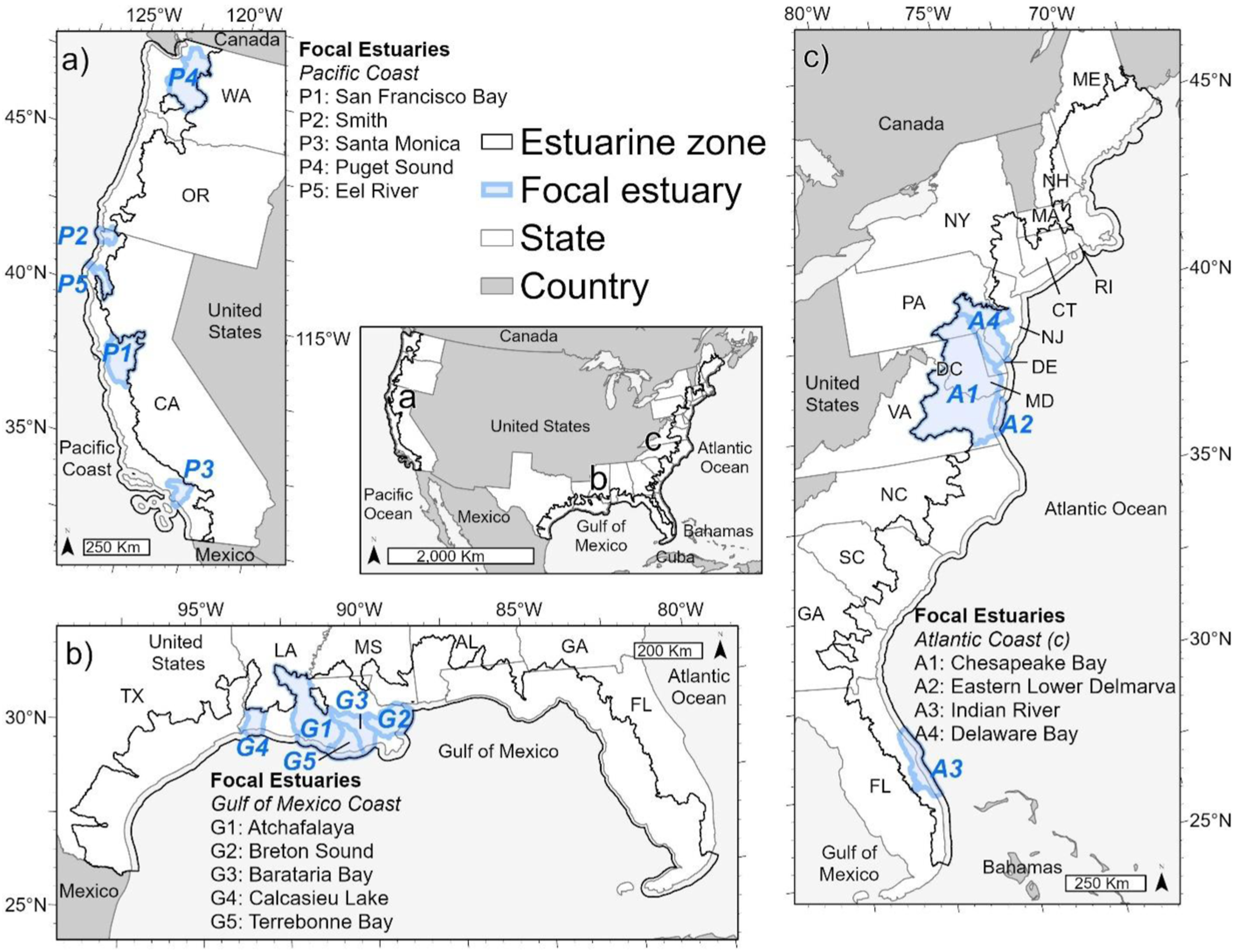

The selected estuaries for wetland change for the Pacific Coast were mainly located in California and include: (1) San Francisco Bay-Delta (California); (2) Smith River (California); (3) Santa Monica Bay (California); (4) Eel River (California); and (5) Puget Sound (Washington). The selected estuaries for wetland change along the northern Gulf of Mexico Coast estuaries were all in Louisiana and include: (1) Atchafalaya; (2) Breton Sound; (3) Barataria Bay; (4) Calcasieu Lake; and (5) Terrebonne Bay. Finally, the selected estuaries for wetland change along the Atlantic Coast estuaries include: (1) Chesapeake Bay (Delaware, District of Columbia, Maryland, Pennsylvania, and Virginia); (2) Eastern Lower Delmarva (Virginia); (3) Indian River (Florida); and (4) Delaware Bay (Maryland, New Jersey, and Pennsylvania).

Vegetation in the estuarine zone along the CONUS includes several types of coastal wetland types: (1) estuarine marshes; (2) mangroves; (3) non-mangrove estuarine woody wetlands; and (4) salt pannes, depending on vegetation coverage and type. Species presence and dominance varies by region and is controlled by abiotic factors such as, climate, hydrology, and geomorphology (Osland et al., 2019). Of the three coasts, the Atlantic Coast has the highest coastal wetland area (9622 km² saltwater [intertidal] and 54,596 km² freshwater) followed by the northern Gulf of Mexico Coast, which has the most saltwater coastal wetlands (13,556 km² saltwater [intertidal] and 48,812 km² freshwater), and the Pacific Coast (2913 km² saltwater [intertidal] and 2249 km² freshwater; Dahl and Stedman, 2013).

Landcover data and change analyses

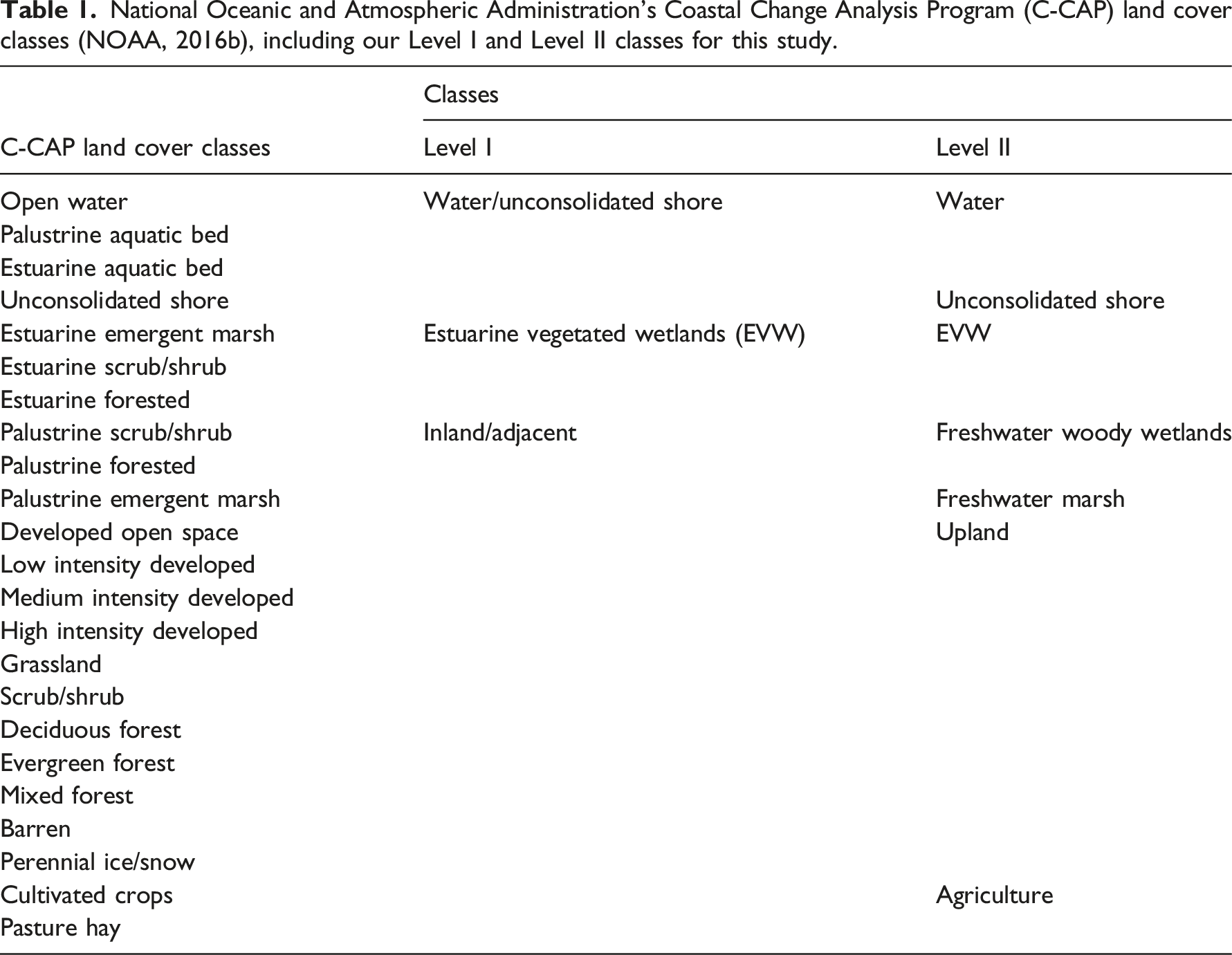
We used a multi-step approach to conduct change analysis (Figure 2). This assessment utilized the C-CAP land cover products from 1996 to 2016. The overall accuracy of these land cover products has been reported to be approximately 85% (NOAA, 2016b). While intermediate landcover products were available between these years, we chose the oldest and newest land cover products and assessed change over a 20-year period. These land cover products are produced at a 30-m spatial resolution and include 23 different land use/land cover classes (Table 1). For our study, we simplified these 23 classes into two different levels. The first level (Level I) included: (1) water/unconsolidated shore; (2) estuarine vegetated wetlands (i.e., vegetated wetlands with a salinity greater than 0.5 ppt); and (3) inland/adjacent. The second level (Level II) retained more thematic detail and included: (1) water; (2) unconsolidated shore; (3) estuarine vegetated wetlands; (4) freshwater woody wetlands; (5) freshwater marsh; (6) upland; and (7) agriculture. See Table 1 for a breakdown of what original C-CAP classes are included in each class at each level.

Figure 2.

Overview of methodology for assessing estuarine vegetated wetland (EVW) change using National Oceanic and Atmospheric Administration’s Coastal Change Analysis Program land cover maps (NOAA, 2016b).

Table 1.

National Oceanic and Atmospheric Administration’s Coastal Change Analysis Program (C-CAP) land cover classes (NOAA, 2016b), including our Level I and Level II classes for this study.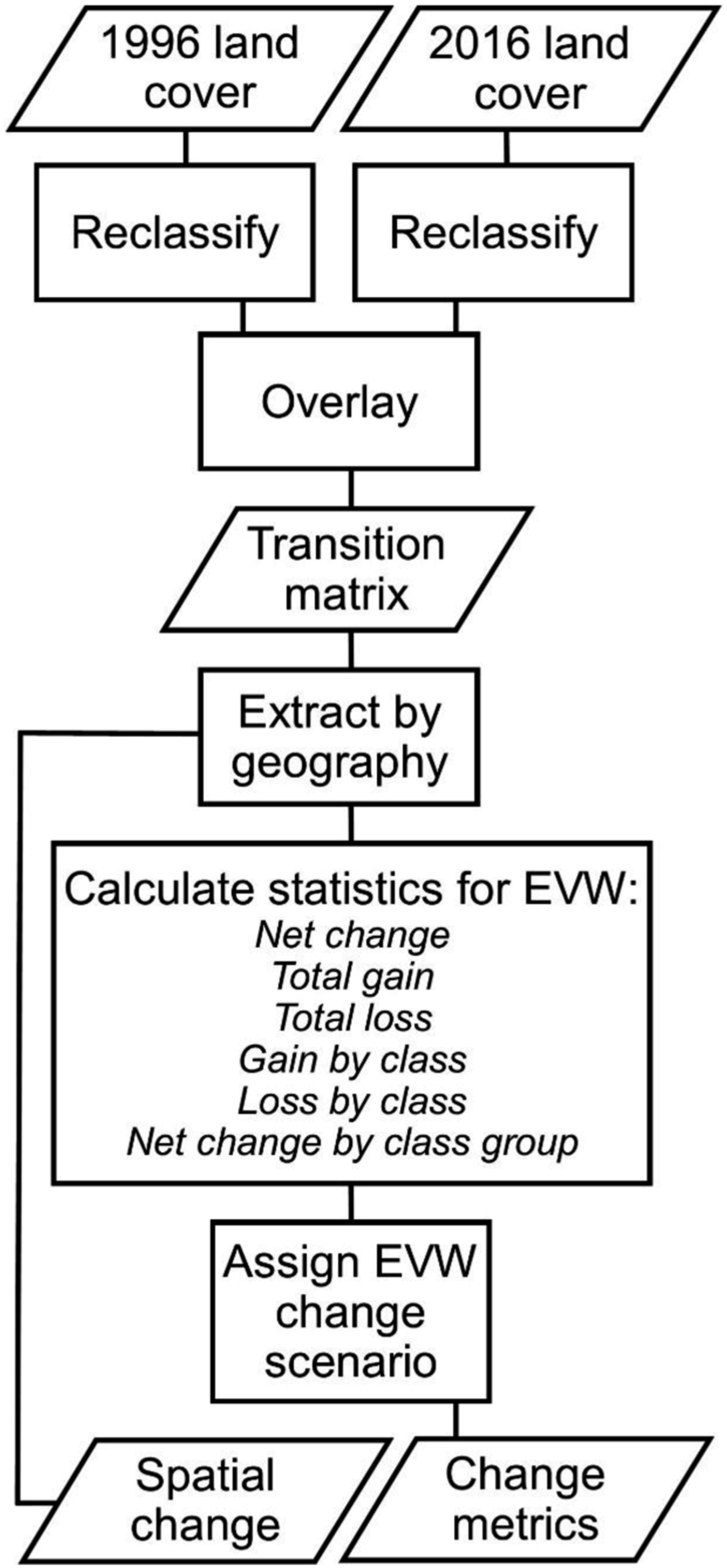

	Classes
C-CAP land cover classes	Level I	Level II
Open water	Water/unconsolidated shore	Water
Palustrine aquatic bed
Estuarine aquatic bed
Unconsolidated shore		Unconsolidated shore
Estuarine emergent marsh	Estuarine vegetated wetlands (EVW)	EVW
Estuarine scrub/shrub
Estuarine forested
Palustrine scrub/shrub	Inland/adjacent	Freshwater woody wetlands
Palustrine forested		Freshwater woody wetlands
Palustrine emergent marsh		Freshwater marsh
Developed open space		Upland
Low intensity developed
Medium intensity developed
High intensity developed
Grassland
Scrub/shrub
Deciduous forest
Evergreen forest
Mixed forest
Barren
Perennial ice/snow
Cultivated crops		Agriculture
Pasture hay		Agriculture

After reclassifying the C-CAP maps, a transition raster and matrix was developed by overlaying the historical and contemporary maps. This transition raster was extracted by spatial area (i.e., full extent, specific coasts, and by estuary [Dale et al., 2022]). Next, the following statistics were calculated for estuarine vegetated wetland area: (1) net estuarine vegetated wetland change; (2) estuarine vegetated wetland gain; (3) estuarine vegetated wetland loss; (4) gain in estuarine vegetated wetlands by class for both levels (i.e., Level I and Level II classes); (5) loss of estuarine vegetated wetlands by class for both levels; and (6) net change in estuarine vegetated wetlands by Level I class.

Change component analysis (Pontius, 2019) can highlight nuanced net change and allocation change, and this approach has been shown to be helpful for studying dynamic environments, such as barrier islands (Enwright et al., 2021). In this study, we developed a simple approach that could highlight overall net area gain and loss and highlight what specific classes contributed to that change. Estuarine vegetated wetland change was assessed by addressing two tasks. The first task was to gauge whether there was a net loss or gain in estuarine vegetated wetland area. The second task was to identify the net area change to other Level I classes (i.e., open water/unconsolidated shore or inland/adjacent).

These tasks were addressed to assign the area to a specific estuarine vegetated wetland change scenario for between 1996 and 2016 (Figure 3). The scenarios include: (1) If there was an overall net loss in estuarine vegetated wetlands with positive gain from open water/unconsolidated shore, then this would signal that land building (i.e., land development through natural processes or restoration) is happening, but the gain is not outpacing overall estuarine vegetated wetland loss due to loss to inland/adjacent classes (LBNO; “land building not outpacing loss”). (2) With a net loss of estuarine vegetated wetlands and a positive gain from inland/adjacent classes, then this would signal that transgression and tidal restoration are occurring, but the gain is not outpacing overall estuarine vegetated wetland loss due to loss to water/unconsolidated shore (TRNO; “transgression/tidal restoration not outpacing loss”). (3) If estuarine vegetated wetlands had a net loss and did not have a positive net change from either of the other Level I classes, then while land building, transgression, and tidal restoration may be occurring, the gain is not at a level that outpaced overall estuarine vegetated wetland loss (LBTRNO; “land building and transgression/tidal restoration not outpacing loss”). (4) If there was an overall net gain in estuarine vegetated wetlands with positive gain from open water/unconsolidated shore, then this would signal that land building may be the main driver in helping to outpace estuarine vegetated wetland loss (LBO; “land building outpacing loss”). (5) With a net gain of estuarine vegetated wetlands and a positive gain from inland/adjacent, then this would signal that transgression and tidal restoration are the main drivers in helping to outpace estuarine vegetated wetland loss (TRO; “transgression/tidal restoration outpacing loss”). (6) With a net gain of estuarine vegetated wetlands and a positive net change for both of the other Level I classes, then land building, transgression, and tidal restoration are the main drivers in helping to outpace estuarine vegetated wetland loss (LBTRO; “land building and transgression/tidal restoration outpacing loss”).

Figure 3.

Estuarine vegetated wetland change scenarios based on overall net loss and gain of estuarine vegetated wetlands and positive net area change for Level I classes (see Table 1).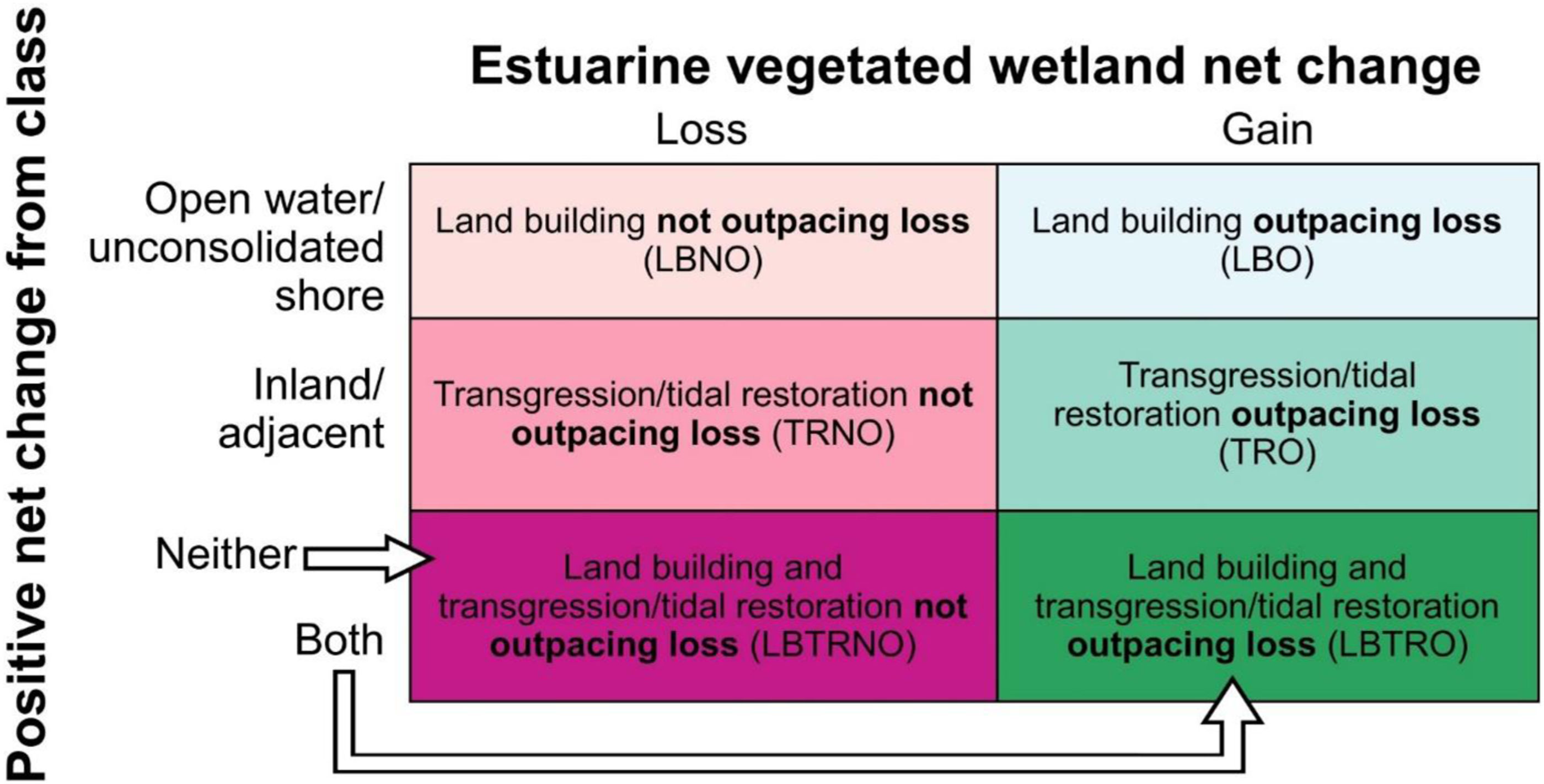

While these change scenarios can provide detailed information on the overall changes, a bivariate scatter plot was used to better understand the relative differences between areas. To do this, we normalized the focal estuaries for net change in estuarine vegetated wetlands from the other Level I classes from 0 to 1 for net gain and 0 to -1 for net loss. Doing so allowed us to interpret the lower left quadrant as LBTRNO and the upper right quadrant to be LBTRO. The upper left quadrant would include TRNO and TRO depending on overall estuarine vegetated wetland net change. The lower right quadrant would include LBNO and LBO depending on overall estuarine vegetated wetland net change.

Maps were then developed to show examples of dynamic areas on each coast (i.e., focal estuaries). These maps depicted areas of gain and loss for estuarine vegetated wetlands along with examples of historical and contemporary imagery. Historical imagery came from the USGS’s National Aerial Photography Program (USGS, 2023) and contemporary imagery came from the US Department of Agriculture’s National Agricultural Imagery Program (USDA, 2023).

Results

Regional estuarine vegetated wetland change

The results of estuarine vegetated wetland change analysis for the CONUS and each coast between 1996 and 2016 showed some areas with gains and others with losses at CONUS and coastline scales (Table 2). At the CONUS-level, there was a net change of estuarine vegetated wetlands equaling −277 km² (gain = 311.6 km²; loss = −589.1 km²). The CONUS had a small net gain for inland/adjacent classes, which led to an estuarine vegetated wetland change scenario of TRNO (Figure 3). For net change for the Level II classes, the largest gain was from freshwater wetlands (38.2 km²) and the largest loss was to water (–300 km²). Along the Pacific Coast, there was a net gain of estuarine vegetated wetlands of 56.8 km² (gain = 77.5 km²; loss = 20.7 km²). This net gain was the largest of the three coasts. The region has a net gain from the other Level I classes, which led to an estuarine vegetated wetland change scenario of LBTRO (Figure 3). For net change for the Level II classes, the largest gain was from freshwater wetlands (29.1 km²) and the largest loss was to agriculture (–1.9 km²). The northern Gulf of Mexico Coast had a net change of estuarine vegetated wetlands of –350.7 km² (gain = 162.3 km²; loss = –513.0 km²). This was the only region that had a net loss for both Level I classes, which led to an estuarine vegetated wetland change scenario of LBTRNO (Figure 3). For net change for the Level II classes, the largest gain was from unconsolidated shore (12.4 km²) and the largest loss was to water (–346.9 km²). Along the Atlantic Coast, there was a net gain of estuarine vegetated wetlands of 16.5 km² (gain = 71.9 km²; loss = –55.4 km²). The region had a net gain for water/unconsolidated shore, which led to an estuarine vegetated wetland change scenario of LBO (Figure 3). For net change for the Level II classes, the largest gain was from water (33.7 km²) and the largest loss was to upland (–21.3 km²).

Table 2.

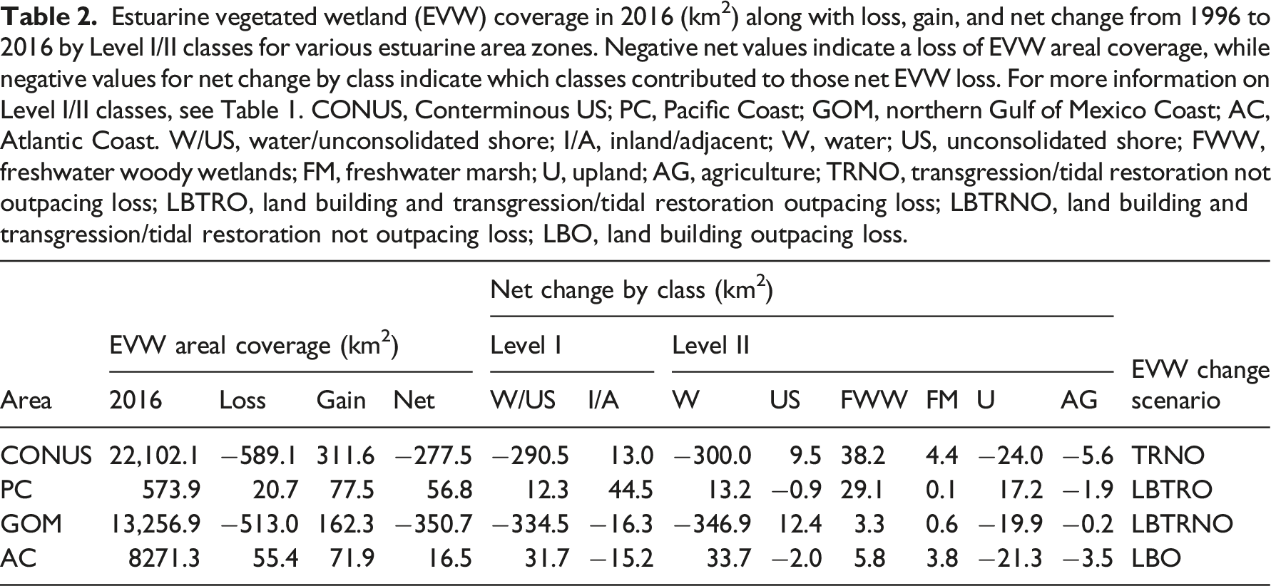
Estuarine vegetated wetland (EVW) coverage in 2016 (km²) along with loss, gain, and net change from 1996 to 2016 by Level I/II classes for various estuarine area zones. Negative net values indicate a loss of EVW areal coverage, while negative values for net change by class indicate which classes contributed to those net EVW loss. For more information on Level I/II classes, see Table 1. CONUS, Conterminous US; PC, Pacific Coast; GOM, northern Gulf of Mexico Coast; AC, Atlantic Coast. W/US, water/unconsolidated shore; I/A, inland/adjacent; W, water; US, unconsolidated shore; FWW, freshwater woody wetlands; FM, freshwater marsh; U, upland; AG, agriculture; TRNO, transgression/tidal restoration not outpacing loss; LBTRO, land building and transgression/tidal restoration outpacing loss; LBTRNO, land building and transgression/tidal restoration not outpacing loss; LBO, land building outpacing loss.

Area					Net change by class (km²)								EVW change scenario
	EVW areal coverage (km²)				Level I		Level II
	2016	Loss	Gain	Net	W/US	I/A	W	US	FWW	FM	U	AG
CONUS	22,102.1	−589.1	311.6	−277.5	−290.5	13.0	−300.0	9.5	38.2	4.4	−24.0	−5.6	TRNO
PC	573.9	20.7	77.5	56.8	12.3	44.5	13.2	−0.9	29.1	0.1	17.2	−1.9	LBTRO
GOM	13,256.9	−513.0	162.3	−350.7	−334.5	−16.3	−346.9	12.4	3.3	0.6	−19.9	−0.2	LBTRNO
AC	8271.3	55.4	71.9	16.5	31.7	−15.2	33.7	−2.0	5.8	3.8	−21.3	−3.5	LBO

Estuarine vegetated wetland change within focal estuaries

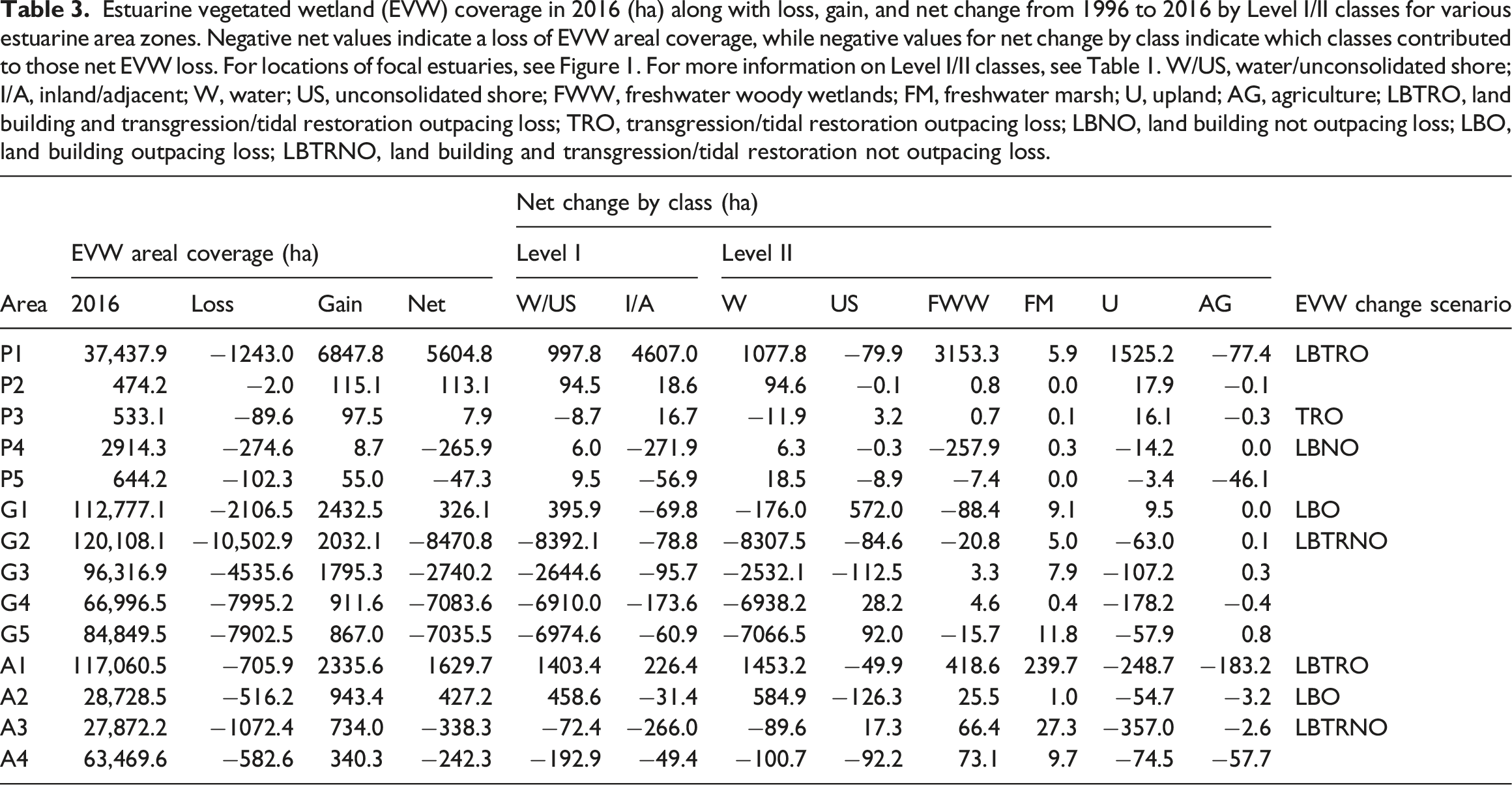
While valuable insights can be gathered from the regional or CONUS analyses, analyses at the estuary-level can provide natural resource managers with information for directing land management practices and restoration actions. Focal estuaries had different estuarine vegetated wetland change scenarios (Table 3). Here we present select estuaries for estuarine vegetated wetland gain and loss for each coast (i.e., Pacific Coast, northern Gulf of Mexico Coast, and Atlantic Coast). For these data and data for all other estuaries, see Han et al. (2023).

Table 3.

Estuarine vegetated wetland (EVW) coverage in 2016 (ha) along with loss, gain, and net change from 1996 to 2016 by Level I/II classes for various estuarine area zones. Negative net values indicate a loss of EVW areal coverage, while negative values for net change by class indicate which classes contributed to those net EVW loss. For locations of focal estuaries, see Figure 1. For more information on Level I/II classes, see Table 1. W/US, water/unconsolidated shore; I/A, inland/adjacent; W, water; US, unconsolidated shore; FWW, freshwater woody wetlands; FM, freshwater marsh; U, upland; AG, agriculture; LBTRO, land building and transgression/tidal restoration outpacing loss; TRO, transgression/tidal restoration outpacing loss; LBNO, land building not outpacing loss; LBO, land building outpacing loss; LBTRNO, land building and transgression/tidal restoration not outpacing loss.

Area	EVW areal coverage (ha)				Net change by class (ha)								EVW change scenario
	EVW areal coverage (ha)				Level I		Level II
	2016	Loss	Gain	Net	W/US	I/A	W	US	FWW	FM	U	AG
P1	37,437.9	−1243.0	6847.8	5604.8	997.8	4607.0	1077.8	−79.9	3153.3	5.9	1525.2	−77.4	LBTRO
P2	474.2	−2.0	115.1	113.1	94.5	18.6	94.6	−0.1	0.8	0.0	17.9	−0.1	LBTRO
P3	533.1	−89.6	97.5	7.9	−8.7	16.7	−11.9	3.2	0.7	0.1	16.1	−0.3	TRO
P4	2914.3	−274.6	8.7	−265.9	6.0	−271.9	6.3	−0.3	−257.9	0.3	−14.2	0.0	LBNO
P5	644.2	−102.3	55.0	−47.3	9.5	−56.9	18.5	−8.9	−7.4	0.0	−3.4	−46.1	LBNO
G1	112,777.1	−2106.5	2432.5	326.1	395.9	−69.8	−176.0	572.0	−88.4	9.1	9.5	0.0	LBO
G2	120,108.1	−10,502.9	2032.1	−8470.8	−8392.1	−78.8	−8307.5	−84.6	−20.8	5.0	−63.0	0.1	LBTRNO
G3	96,316.9	−4535.6	1795.3	−2740.2	−2644.6	−95.7	−2532.1	−112.5	3.3	7.9	−107.2	0.3
G4	66,996.5	−7995.2	911.6	−7083.6	−6910.0	−173.6	−6938.2	28.2	4.6	0.4	−178.2	−0.4
G5	84,849.5	−7902.5	867.0	−7035.5	−6974.6	−60.9	−7066.5	92.0	−15.7	11.8	−57.9	0.8
A1	117,060.5	−705.9	2335.6	1629.7	1403.4	226.4	1453.2	−49.9	418.6	239.7	−248.7	−183.2	LBTRO
A2	28,728.5	−516.2	943.4	427.2	458.6	−31.4	584.9	−126.3	25.5	1.0	−54.7	−3.2	LBO
A3	27,872.2	−1072.4	734.0	−338.3	−72.4	−266.0	−89.6	17.3	66.4	27.3	−357.0	−2.6	LBTRNO
A4	63,469.6	−582.6	340.3	−242.3	−192.9	−49.4	−100.7	−92.2	73.1	9.7	−74.5	−57.7	LBTRNO

For the estuaries with an overall net gain of estuarine vegetated wetlands, we found that that the Atchafalaya (G1, Gulf Coast) and Eastern Lower Delmarva (A2, Atlantic Coast) estuaries had an estuarine vegetated wetland change scenario of LBO. Both regions had a large net gain of estuarine vegetated wetlands from water/unconsolidated shore; however, the Atchafalaya estuary gained mostly from unconsolidated shore (572 ha) and the Eastern Lower Delmarva estuary gained from mostly from water (584.9 ha). Santa Monica Bay (P3, Pacific Coast) was the only estuary to have an estuarine vegetated wetland change scenario of TRO. This estuary had a small net gain (7.9 ha) with a gain coming from inland/adjacent classes (16.7 ha), mainly upland (16.1 ha). The San Francisco Bay-Delta (P1, Pacific Coast), Smith River (P2, Pacific Coast), and Chesapeake Bay (A1, Atlantic Coast) estuaries had an estuarine vegetated wetland change scenario of LBTRO. Of the three, the San Francisco Bay-Delta and Chesapeake Bay estuaries had a large net gain of estuarine vegetated wetlands. The San Francisco Bay-Delta estuary had a much larger net gain inland/adjacent classes (4607 ha) compared to water/unconsolidated shore (997.8 ha). This gain was mainly from freshwater woody wetlands (3153.3 ha) and upland (1525.2 ha). Figure 4 shows examples of estuarine vegetated wetland gain and loss for areas in the San Francisco Bay-Delta estuary. Examples of extensive estuarine vegetated wetland gain were found in the estuary (Figure 4(a)–(c)); after investigation it was determined that this is an area that has undergone restoration efforts to reintroduce tidal action into former diked salt production ponds along the Coyote Creek (South Bay Salt Pond Restoration Project, 2023).

Figure 4.

Examples of estuarine vegetated wetland (EVW) gain and loss from 1996 to 2016 for the San Francisco Bay-Delta (California) focal estuary on the Pacific Coast (P1; Figure 1) from the National Oceanic and Atmospheric Administration’s Coastal Change Analysis Program land cover maps. An example of marsh creation is shown in panes a–c. Panes d–f show a marsh creation site where the southern portion of the site shows up as EVW gain, but the northern portion incorrectly shows up as EVW loss. Historical images are from US Geological Survey’s (USGS) National Aerial Photography Program (USGS, 2023) from August 1998 (b) and USGS Single Aerial Frames from February 1996 (e). Contemporary imagery (a, c, d, and f) is from the US Department of Agriculture’s National Agricultural Imagery Program (USDA, 2023) from May 2016 (a), (c) to June 2016 (d), (f). The basemap imagery in overview map is from Earthstar Geographics.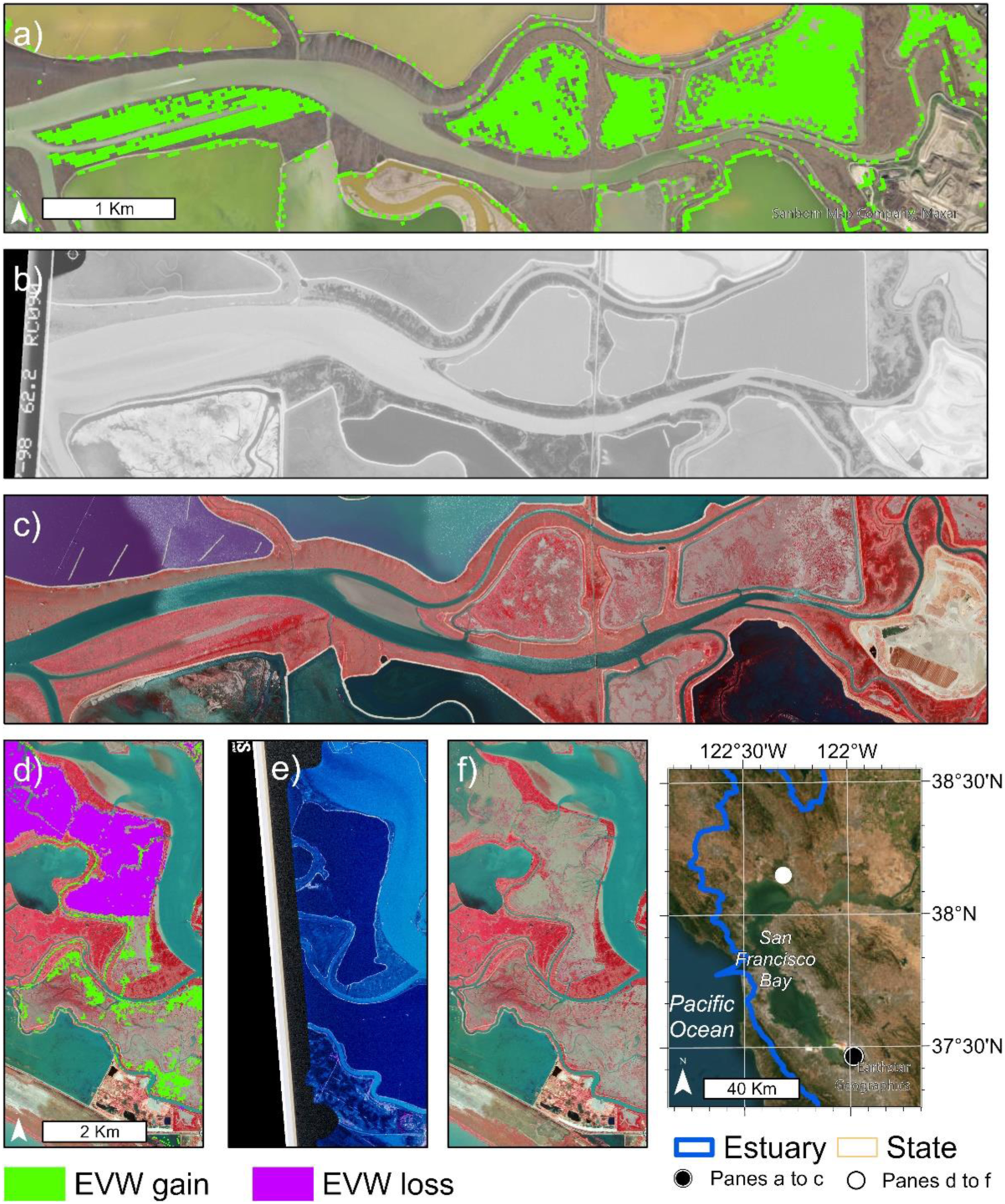

However, some restoration areas appeared to be misclassified as estuarine vegetated wetland loss (Figure 4(d)–(f)). After further investigation, it was determined this area is part of the Napa-Sonoma Marshes Wildlife Area which has ongoing restoration efforts to reintroduce tidal action into former salt ponds, with area breached to tidal waters in 2006 (Brand et al., 2012). This classification could be due to varying tidal levels during image capture, but it is difficult to know exactly why this area was classified by C-CAP as estuarine vegetated wetland in 1996 because at that time it was diked fallow fields and historic salt ponds (Brand et al., 2012) and non-estuarine vegetated wetland in 2016 when breaching occurred in 2006 (Figure 4(d)–(f)). In contrast, Chesapeake Bay had a higher net gain from water/unconsolidated shore (1403.4 ha) than inland/adjacent classes (226.4 ha). The net gain in water/unconsolidated shore was from water (1453.2 ha). Figure 5 shows examples of estuarine vegetated wetland gain and loss for an area in the Chesapeake Bay estuary with an example of gain from water (Figure 5 d–f).

Figure 5.

Examples of estuarine vegetated wetland (EVW) gain and loss from 1996 to 2016 for Chesapeake Bay (Delaware, Maryland, Pennsylvania, and Virginia) focal estuary on the Atlantic Coast (A1; Figure 1) from the National Oceanic and Atmospheric Administration’s Coastal Change Analysis Program land cover maps. Pane a–c shows loss along the marsh edge and gain from areas previously classified as freshwater wetlands. Pane d–f highlights gain in an impounded wetland. Historical images are from US Geological Survey’s National Aerial Photography Program (USGS, 2023) from March 1998 (b), (e). Contemporary imagery is from the US Department of Agriculture’s National Agricultural Imagery Program (USDA, 2023) from June 2017 (a, c, d, and f). The basemap imagery in overview map is from Earthstar Geographics.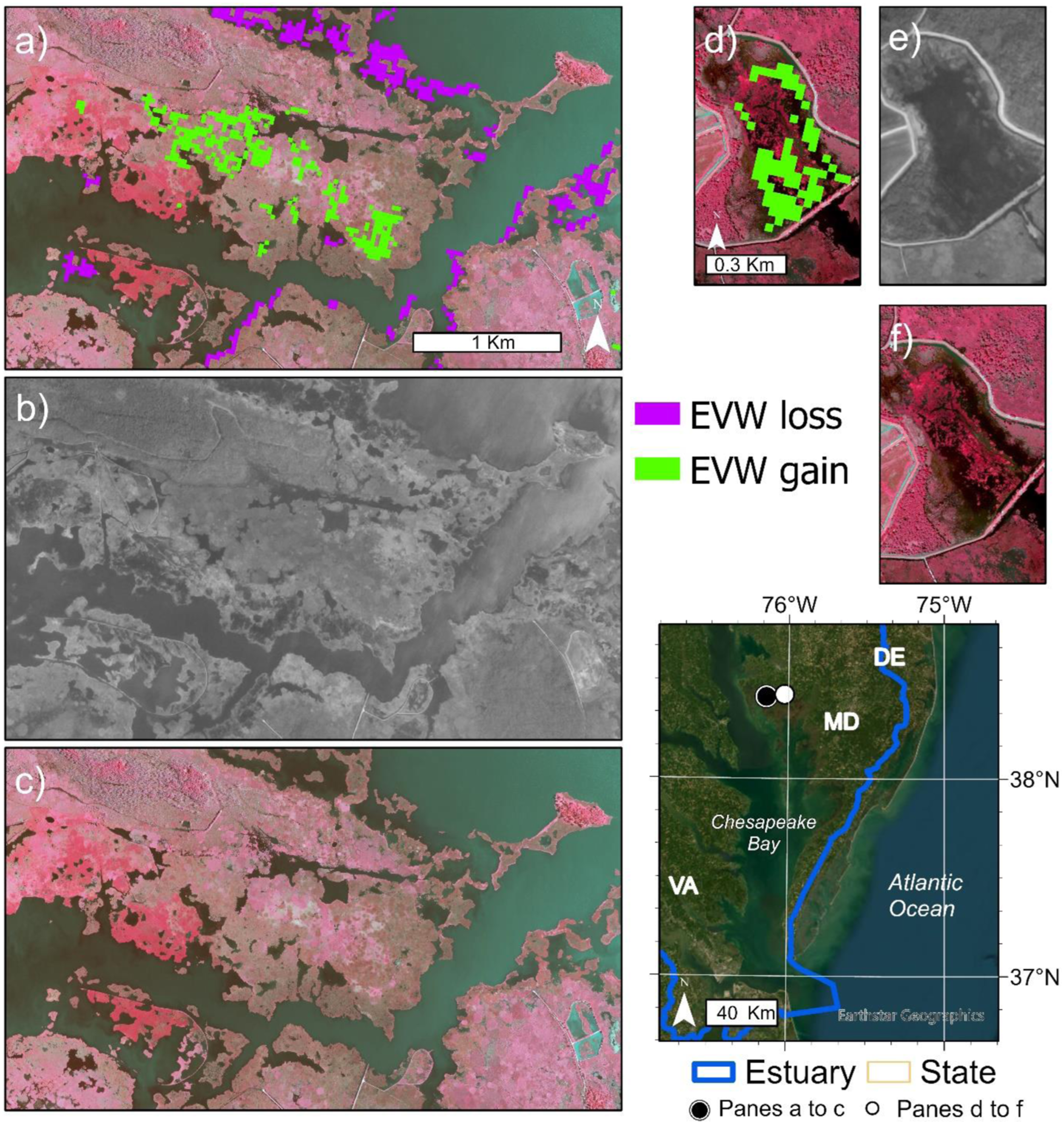

For estuaries with a net loss of estuarine vegetated wetland, we found Puget Sound (P4, Pacific Coast) and Eel River (P5, Pacific Coast) had an estuarine vegetated wetland change scenario of LBNO. Both estuaries had a small net gain of estuarine vegetated wetlands from the water/unconsolidated shore class, but this gain did not offset the large amount of loss in inland/adjacent classes. For the Puget Sound estuary, most of the estuarine vegetated wetland loss was to freshwater woody wetlands (257.9 ha), whereas most of the estuarine vegetated wetland loss was to agriculture (46.1 ha) for the Eel River estuary. No estuaries had the TRNO estuarine vegetated wetland change scenario. Four estuaries along the northern Gulf of Mexico Coast and two estuaries along the Atlantic Coast exhibited the LBTRNO estuarine vegetated wetland change scenario. The northern Gulf of Mexico Coast estuaries in this estuarine vegetated wetland change scenario included Breton Sound (G2), Barataria Bay (G3), Calcasieu Lake (G4), and Terrebonne Bay (G5). These estuaries all have a large amount of net loss of estuarine vegetated wetlands to the water/unconsolidated shore classes (range: 2644.6 ha to 8392.1 ha), with this loss largely coming from the water class. These estuaries also have a net loss of estuarine vegetated wetlands to inland/adjacent classes, but these changes were much lower (range: 60.9 ha to 173.6 ha). Figure 6 shows examples of estuarine vegetated wetland gain and loss for an area in the Breton Sound estuary. Although some gains were shown, there was extensive loss of estuarine vegetated wetlands to water. The Atlantic Coast estuaries with the LBTRNO estuarine vegetated wetland change scenario included Indian River and Delaware Bay. The Indian River estuary had a much higher net loss of estuarine vegetated wetlands to inland/adjacent (266 ha) compared to water/unconsolidated shore (72.4 ha). In contrast, the Delaware Bay estuary had much higher loss of estuarine vegetated wetlands to water/unconsolidated shore (192.9 ha) than inland/adjacent (49.4 ha).

Figure 6.

Examples of estuarine vegetated wetland (EVW) gain and loss from 1996 to 2016 Breton Sound (Louisiana) focal estuary on the northern Gulf of Mexico Coast (G2; Figure 1) from the National Oceanic and Atmospheric Administration’s Coastal Change Analysis Program land cover maps. A high concentration of marsh loss is shown in pane a–c. Pane d–f highlights areas of gain and loss a little to northwest. Historical images are from US Geological Survey’s National Aerial Photography Program (USGS, 2023) from January 1994 (b), (e). Contemporary imagery is from the US Department of Agriculture’s National Agricultural Imagery Program (USDA, 2023) from September 2017 (a, c, d, and f). The basemap imagery in overview map is from Earthstar Geographics.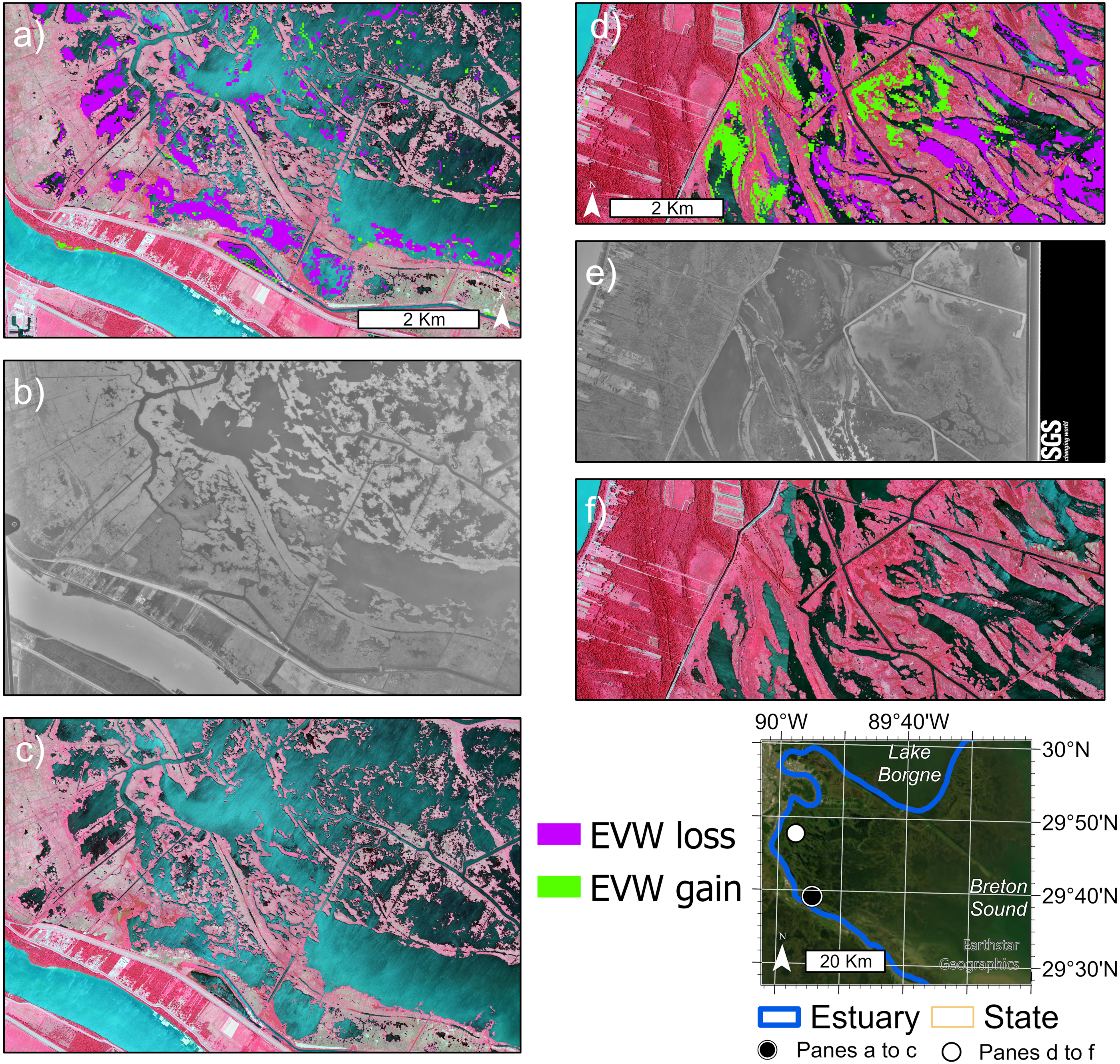

Discussion

National change assessment

The goal of this framework was to provide a simple set of metrics that can be used to understand the trajectory of estuarine vegetated wetlands over time (Figure 3). In our study, the different estuarine vegetated wetland change scenarios highlight the change that was captured in moderate-resolution land cover datasets over the past 20 years. Observing spatiotemporal estuarine vegetated wetland change can provide insights to land managers for making future-focused land management decisions. The adaptive capacity for coastal wetlands in response to sea-level rise impacts is known to be related to elevation and coastal slope (Osland et al., 2022) and sediment availability (Saintilan et al., 2022). The use of estuarine vegetated wetland change scenarios can provide insight into how estuarine vegetated wetlands are responding to sea-level rise in estuaries over time.

As a proof-of-concept, our framework was only applied to two snapshots; however, the framework can be used to conduct repeat assessments over time to capture the non-linear nature of coastal wetland changes from sea-level rise (Sweet et al., 2022), precipitation (Osland et al., 2014; Wang et al., 2022), sediment availability (Morris et al., 2002), winter temperatures (Osland et al., 2021), extreme storm frequency (Cahoon, 2006; Thorne et al., 2022), and coastal wetland restoration (Williams and Faber, 2001; Zhao et al., 2016; Bertolini and da Mosto, 2021). Repeated observations of these change metrics over time can provide important insights into critical thresholds for coastal wetland adaptive capacity and may improve the predictive power of wetland ecosystem modeling. Generally, the southeastern US has expansive room for the migration of estuarine vegetated wetlands into upslope/adjacent lands, whereas the northern Atlantic Coast and Pacific Coast have much less room due to steeper topography and developed lands (Osland et al., 2022). However, most of the potential estuarine wetland vegetation migration space along the northern Gulf of Mexico and southern Atlantic coasts is currently classified as palustrine wetlands (i.e., freshwater forests and marshes) (Osland et al., 2022). Thus, the potential landward migration of the saline vegetation classes (i.e., vegetated “estuarine wetlands”) would be at the expense of vegetated freshwater wetlands (i.e., vegetated “palustrine wetlands”). With projected sea-level rise and predicted increases in the frequency of high tide flooding events, there is an expectation that the estuarine vegetated wetland change scenarios may increasingly show the contribution of upland transgression to the future change analyses, especially along the northern Gulf of Mexico Coast (Thompson et al., 2021).

The metrics produced in this study can be used to provide land managers and other decision-makers with insights for making future-focused management decisions using the resist-accept-direct (RAD) framework (Schuurman et al., 2020). For example, this information can highlight where change could be resisted (e.g., restoration actions to avoid wetland loss, sediment addition), accepted (i.e., accepting upslope migration or localized wetland loss), or how and where change could be directed (e.g., tidal restoration of impounded wetlands or enhancing migration corridor connectivity). Sudol et al. (2023) presented an application of the RAD framework with agricultural producers in the Chesapeake Bay for addressing sea-level rise impacts. While we only applied this framework to estuarine vegetated wetlands, it could also be used to highlight changes in freshwater wetlands and other coastal ecosystems. Given that the landward migration of tidal saline wetlands is predicted to occur primarily at the expense of adjacent freshwater wetlands, this could be an important future step to highlight the full transformation of coastal ecosystems within an estuary in response to sea-level rise (Osland et al., 2022).

Relative change at the estuary-level

The estuary-level assessments can provide helpful insights for local decision-making. Expressing these overall net changes for the two Level I classes as a bivariate panel plot allows for comparison of estuaries by coast and within estuarine vegetated wetland change scenarios (Figure 7). The bi-plot can show how wetlands are adapting to climate change associated sea-level rise and assist with the comparison of areas with different spatial extents. While our study focused on estuaries, this approach could be used to assess the metrics of other areas (e.g., management units, wildlife refuges, parks, and preserves). For example, we can see how different the San Francisco Bay-Delta (P1), Atchafalaya (G1), and Chesapeake Bay (A1) estuaries are from other estuaries along the same coasts. Additionally, normalizing the results allows for the relative comparison between estuaries with the same estuarine vegetated wetland change scenario. For instance, the San Francisco Bay-Delta estuary had the highest gain from the other Level I classes, whereas the Chesapeake Bay estuary had the highest gain from the water/unconsolidated class.

Figure 7.

Comparison of net change for the inland class (i.e., upland land cover and freshwater wetlands) and the water/unconsolidated shore class for focal estuaries located in the Atlantic Coast (A), northern Gulf of Mexico Coast (G), and Pacific Coast (P). Negative values indicate loss of estuarine vegetated wetlands to class and positive values indicate gain of estuarine vegetated wetlands from class. For locations of focal estuaries, see Figure 1. Color coding is based on scenarios: LBTRNO, Land building and transgression/tidal restoration not outplacing loss; TRNO, Transgression and tidal restoration not outpacing loss; LBNO, Land building not outpacing loss; LBTRO, Land building, transgression, and tidal restoration outplacing loss; TRO, Transgression and tidal restoration outpacing loss; LBO, Land building outpacing loss.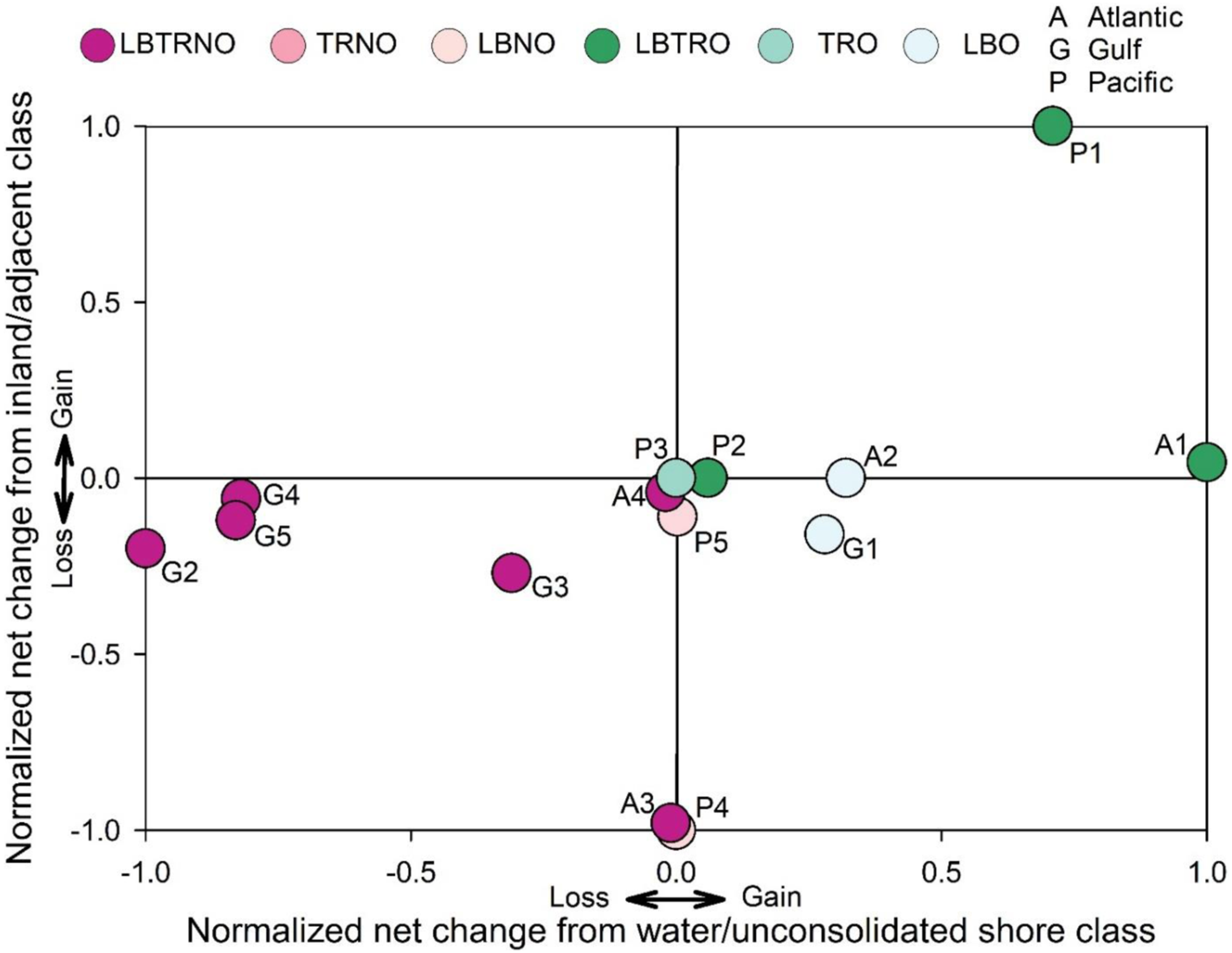

While our study focused on abundance of wetland change, exploring change relative to the estuary size may be important. This information can be helpful for management objectives or research questions focused on finding areas that have a limited coverage of wetlands that are experiencing a lot of change. To address these alternative questions, we added statistics for net change that are relative to estuary area and initial (i.e., 1996) estuarine vegetated wetland area to the data release associated with this study (Han et al., 2023).

Comparison with other studies

A robust accuracy assessment of change was beyond the scope of this study because an acceptable accuracy assessment would require utilizing high-resolution readily available imagery for both dates. Specifically, the separation of estuarine vegetated wetlands and upslope/adjacent wetlands from historical imagery would be challenging and subjective (e.g., Scheider et al., 2018). Due to the feasibility challenges associated with this level of an assessment, we relied on historical and contemporary imagery comparisons (Figures 4 –6) and general comparisons with existing national coastal wetland change assessments and local studies to provide a qualitative assessment of the approach. Our rationale for a qualitative approach is that there can be many factors that influence the results of a remotely sensed classification of wetlands, such as classification method, spatial resolution of data sources, temporal resolution of data sources, thematic detail of assessments, temporal differences in studies, geographic boundary differences, limited data availability of classification products for ensuring the comparison is appropriate, and the non-linear nature of coastal wetland vegetation change.

The framework used in this study is complementary to other change assessments via NWI Status and Trends analyses, which produce regional change estimates from mapping change by using photointerpretation and field verification in randomly sampled areas (USFWS, 2020). Despite different methods, the findings from this study track result from the US Fish and Wildlife Service’s Status and Trends analysis from 2004 to 2009 (Dahl and Stedman, 2013). For CONUS, there was a net loss of estuarine vegetated wetlands, and the dominant estuarine vegetated wetland change scenario was TRNO. Similar to the 2004 to 2009 Status and Trends analysis, we also found regional variability for estuarine vegetated wetland losses along the northern Gulf of Mexico Coast and small estuarine vegetated wetland gains in the other two coasts.

Generally, our findings also agree with local, site-specific studies. For instance, we found southeast Louisiana to have several estuaries that have a high net loss of estuarine vegetated wetlands and an estuarine vegetated wetland change scenario of LBTRNO (Table 3; Figure 7), which agrees with what has been found in long-term satellite-based land area change analyses for this area (Couvillion et al., 2017; Potter et al., 2020; Jensen et al., 2022). The extreme loss of estuarine vegetated wetlands in southeastern Louisiana is due to high relative sea-level rise (Sweet et al., 2022), subsidence from deltaic deposits (Twilley et al., 2016), and limited sediment availability for wetland accretion due to Mississippi River levees (Jensen et al., 2022). Similarly, our results of a gain of estuarine vegetated wetlands in the Atchafalaya Basin from deltaic progradation (Twilley et al., 2019) are in agreement with findings by Couvillion et al. (2017) and Jensen et al. (2022).

We found the Chesapeake Bay had an overall net gain (A1; A2; A4). When pooled, the Chesapeake Bay estuary had an estuarine vegetated wetland change scenario of LBTRO with most of the gain coming from conversion of water to estuarine vegetated wetlands (net gain of 1937 ha) and a minor net gain from conversion of upslope/adjacent classes (net gain 145.6 ha) with the gains coming from freshwater woody wetlands and freshwater marsh. Researchers recently highlighted how upland to wetland conversion compensated for wetland losses over the recent history in the Chesapeake Bay (1846 to 2013; Scheider et al., 2018). Both our work and Scheider et al. (2018) highlight regional variation within the Chesapeake Bay. Generally, there was more gain from upslope/adjacent classes and overall net gain on the western side of the Chesapeake Bay. Differences between our study and the results by Scheneider et al. (2018) are likely due to the much larger timespan when using National Ocean Service topographic sheets (“T-sheets”) from as far back as 1846 to 1912. Scheneider et al. (2018) may also have been able to detect smaller changes by manually digitizing marsh and other classes from very high-resolution aerial imagery (0.15 m) from 2013. For the Pacific Coast, we found that our metrics were able to detect net gain of estuarine vegetated wetlands in the San Francisco Bay-Delta estuary, which are predicted to be due from extensive restoration activities beginning in the early 1970s (Williams and Faber, 2001). Due to the steep slopes and urbanization, restoration will be one of the main approaches for offsetting estuarine vegetated wetland loss in San Francisco Bay (Williams and Faber, 2001; Thorne et al., 2018; San Francisco Estuary Blueprint, 2022).

Importance of local, targeted wetland change analyses

Although the framework utilized in this study can be conducted at the national and regional level, information produced from this study can be enhanced by targeted, local analyses. For example, researchers have observed and quantified the development of dead or dying forests in North Carolina (i.e., “ghost forests,” which describes previously forested areas that now are marked with standing dead trees and fallen tree trunks) over a 35-year period using Landsat satellite imagery (Ury et al., 2021), upslope migration in central California (Wasson et al., 2013), widespread coastal wetland losses and concentrated gains (in active deltas) in coastal Louisiana (Couvillion et al., 2017), and wetland changes in Chesapeake Bay (Scheider et al., 2018). As previously mentioned, the overall accuracy of C-CAP’s national land cover data is around 85%. Consequently, some changes detected and/or lack of changes observed may be erroneous. Another benefit of local change analyses is that these products may have a higher overall accuracy than national products given the targeted focus on a specific area and development of customized classification approaches. In summary, while the standardized nature of national products helps with scaling up to large regions and comparison across areas, local case studies like the ones highlighted here will continue to be important for providing detailed information at local scales.

Wetland mapping advancements for observing anticipated changes

While this study demonstrated the utility of the proposed framework, C-CAP’s past reliance on historical data and spatial resolution may need to be enhanced to increase the ability to detect changes between upland/adjacent classes (i.e., upland and palustrine), estuarine wetlands, and water/unconsolidated shore classes. Specifically, it is important that the methodology used to develop the national maps utilizes contemporary remote sensing and innovative algorithms in order to detect changes based on contemporary remotely sensed observations. In addition to better delineating palustrine and estuarine wetland zones, advancements could be made by increasing the spatial resolution of the products. NOAA has already begun addressing spatial resolution limitations through the development of regionally available high-resolution C-CAP maps (1-m spatial resolution). These high-resolution land cover maps can provide a baseline that would be more capable of detecting narrow coastal wetland change like marsh edge erosion and migration into upslope and adjacent cover types, especially when migration occurs in narrow bands due to short time intervals or steep slopes. In other words, these data will be able to detect change that is undetectable in moderate-resolution products (i.e., 30-m C-CAP) and can help reduce the underestimation of change for future implementations of this approach. Another potential improvement would be the refinement of the current vegetation classes to better reflect estuary boundaries (Brophy et al., 2019). For example, coastal freshwater wetlands exposed to oceanic water in the upper portion of the estuary (e.g., tidal freshwater marshes and forests) are likely defined by C-CAP as palustrine wetlands and not included in the estuarine vegetated wetland class. Expanding the approach used in this study to include estuarine vegetated wetlands and freshwater tidal wetlands could provide a more complete picture of changes to the extent of wetlands within an estuary. The subsequent sections highlight approaches that could be used to advance and complement future national land cover mapping products.

Wetland inundation mapping

As previously mentioned, we used the estuarine wetland class, which have a salinity greater than 0.5 ppt (Cowardin et al., 1979), to represent estuarine wetlands. Estuarine wetlands in this classification include areas that are regularly exposed to saline waters (i.e., from high tides) and irregularly exposed to saline water (i.e., less than daily though regular tides, perigean spring tides, wind-induced water fluctuations, and storms). This section highlights recent remote sensing advancements that have allowed researchers to directly detect flooding or estimate the likelihood of oceanic flooding. These types of approaches could be helpful for refining estuarine boundaries and better identifying the palustrine–estuarine ecotone for future national land cover mapping efforts, especially as the frequency of high tide flooding events increase over the next several decades with accelerated sea-level rise (Thompson et al., 2021; Sweet et al., 2022).

Researchers have developed metrics for using optical satellite imagery for detecting tidal flooding in wetlands. O’Connell et al. (2017) developed the Tidal Marsh Inundation Index (TMII), which is an index that can be applied to time series of MODIS (Moderate-Resolution Imaging Spectroradiometer) satellite imagery data. When compared to in situ observations, the TMII classified coastal flooding with a 77 to 80% accuracy for the Georgia and Massachusetts sites. Narron et al. (2022) built upon this approach to develop the “Flooding in Landsat across tidal systems (FLATS)” algorithm. This approach used Landsat 8 imagery to produce a higher spatial resolution product (30 m) for determining tidal inundation and frequency of flooding. FLATS correctly identified true flooded pixels with an accuracy of 81%. TMII and FLATS both utilize the normalized difference water index (NDWI; Gao, 1996) and phenology information.

Synthetic aperture radar (SAR) imagery has many advantages over optical satellite imagery, including the ability to collect data with cloud cover and during both day and night (Musa et al., 2015; Goumehei et al., 2019). Thresholding methods have been used successfully with SAR imagery to identify and map surface water (Huang et al., 2017). Similar thresholding can be used to map inundation in wetlands after storm events (Rangoonwala et al., 2016; Yu and Gao, 2023) and during typical tides (Chaouch et al., 2012; Lamb et al., 2019). The upcoming launch of the National Aeronautics and Space Administration and Indian Space Research Organization’ NISAR satellite (the proposed launch is currently in 2024) is predicted to enhance the ability for researchers to detect flooding in vegetated areas (Ottinger and Kuenzer, 2020). NISAR will make L-band SAR freely available globally with a spatial resolution of 3 to 10 m and a 12-day revisit period.

Other studies have used light detection and ranging data and elevation error estimates to map the probability of an area being below specific water levels (Enwright et al., 2018, 2023; Holmquist et al., 2018; Holmquist and Windham-Myers, 2022). For the CONUS, Holmquist et al. (2018) used the best available elevation data and uncertainty information (i.e., elevation error and tidal datum transformation error) to develop a probabilistic map of areas falling below the mean higher high water springs tidal datum, a map of relative tidal elevation, and a probabilistic map of regularly flooded wetlands (i.e., elevation below mean high water). For the Gulf of Mexico, Enwright et al. (2023) used the best available elevation data and uncertainty information (i.e., elevation error, tidal datum transformation error, and flood threshold uncertainty) to develop a probabilistic map of irregularly flooded wetlands.

Higher resolutions and image processing

Incorporating higher spatial resolution data, higher temporal resolution data, and image processing advancements are potential ways to increase the accuracy and utility of information from national wetland mapping programs. Recent advancements in high-resolution commercial satellite imagery may enable the production of regional high-resolution imagery with an increased temporal frequency. Additionally, national aerial imagery programs, such as the US Department of Agriculture’s National Agriculture Imagery Program, have also been advancing and are now acquiring very-high-resolution imagery (i.e., 0.3 m). As previously mentioned, increased spatial resolution should help reduce issues with misclassification of estuarine vegetated loss (Figure, 4e-f), allow the detection of edge erosion, marsh collapse, and migration of wetland zones into upslope/adjacent land cover types, especially when these changes occur in narrow zones. However, the increased spatial resolution may also introduce new challenges. For example, the use of high-resolution commercial satellite data for national land cover mapping with the objective of future change assessment may warrant addressing specific considerations, particularly ensuring accurate geo-registration between mapping efforts (Frazier and Hemingway, 2021). Additionally, higher resolution imagery can increase within-class spectral variabilities, the “H-resolution problem” (Hay et al., 1996). Working with high-resolution aerial imagery may require overcoming additional issues related to color balancing between adjacent flight lines and inconsistencies between digital numbers between image acquisitions (Maxwell et al., 2017). Of particular importance for coastal mapping is the lack of tide-coordination for coastal areas, which could result in water level varying by area.

These challenges may lead to the need to explore different land cover mapping methodologies to create products that can inform decision-making. One approach that has shown to help with the challenges of high-resolution imagery is the use of geographic object-based image analysis (GEOBIA; Blaschke et al., 2014). GEOBIA is an efficient approach that segments high-resolution imagery into objects and then classifies objects instead of individual pixels. Due to the advancement of computational capabilities (Christophe et al., 2011), another emerging research direction in remote sensing is the use of deep convolutional neural networks (“deep learning”) for semantic mapping (i.e., classifying individual pixels in an image; Kattenborn et al., 2021). Of particular interest for coastal mapping is the use of recurrent convolutional neural networks, which are capable of learning temporal patterns in a data time series. Gray et al. (2021) tested a variety of classifiers for mapping general coastal land cover types over 20 years of Landsat imagery and found that recurrent convolutional neural networks outperformed deep convolutional neural networks and other commonly used machine learning algorithms, such as random forest and support vector machine. Morgan et al. (2022) found similar results when comparing a convolutional neural network with random forest and support vector machine algorithms that mapped broad coastal land cover types, such as marsh, water, forest, non-vegetated, and agriculture/grass and urban for Beaufort County, South Carolina, using 1-m aerial imagery. While computational efficiency is increasing (Christophe et al., 2011), the convolutional neural network took about 46 h to produce the classification compared to 5 h each for support vector machine and random forest—an increase of 820% in compute time—using a high-end GIS workstation. Another challenge for semantic mapping with deep convolutional neural networks is the need for large amounts of training data. In response, expansive libraries of training data (i.e., labeled images and points) have been built that can be used for training and tuning deep convolutional neural networks or other algorithms (Murray et al., 2022; Buscombe et al., 2023).

Condition-based mapping

The framework highlighted in this study can be used to better understand coastal wetland change from land cover data; however, observing condition changes (i.e., increase/decrease in plant greenness, wetness, brightness) can help point to impending land cover changes. Yang et al. (2022) developed a novel automated approach for tracking coastal wetland changes called “detection and characterization of coastal tidal wetlands change” (DECODE). Their approach was used to detect land cover changes (i.e., water, vegetated wetlands, other [unvegetated and upland]) and condition changes, which were detectable changes using spectral bands and greenness, wetness, and brightness information from Landsat imagery in the northeastern US. Cover change had a user's and producer's accuracy of around 68% and 80%, respectively, whereas condition change had a user’s and producer’s accuracy of around 80% and 97%, respectively. For specific wetland complexes/units, the unvegetated to vegetated ratio (UVVR) has been found to be correlated with sediment budgets and sea-level rise (Ganju et al., 2017). UVVR has been mapped with high-resolution aerial imagery and Landsat satellite imagery (Ganju et al., 2022). Approaches like DECODE and UVVR can be used to provide robust condition-based information to land managers that can highlight trajectories of land cover types within coastal wetlands.

Conclusion

This study highlights how standardized wetland maps can be used to assess and understand estuarine vegetated wetland area changes. The straightforward approach we present here uses overall net gain/loss of estuarine vegetated wetland areas and what land cover types contribute to that change to determine an estuarine vegetated wetland change scenario. Specifically, the estuarine vegetated wetland change scenarios highlight whether or not wetlands in a given area were keeping up with loss and whether the contribution was from transgression/restoration or land building or both. The estuarine vegetated wetland change scenarios, which can be assessed for spatial scale (e.g., entire coast or estuary), varied by major US coastline and estuary. Collectively, this information can be used by natural resource managers and other decision-makers to better understand how estuarine vegetated wetland change is occurring across multiple scales. This information could be helpful for making future-focused decisions regarding restoration and provide insight into the response of estuarine vegetated wetlands to sea-level rise in a specific estuary. To accurately observe and quantify changes to estuarine vegetated wetlands, it may be important for national mapping programs to utilize methods that use contemporary information for separating different kinds of wetlands (e.g., estuarine and palustrine wetlands; different kinds of wetland forests, marshes, and salt flats). Synthetic aperture radar, optical satellite imagery, and elevation data may be helpful for observing or estimating inundation regimes for coastal wetlands. Additionally, increasing the spatial and temporal resolution of future national mapping efforts may allow for a more robust understanding of coastal wetland change. Processing higher resolution data more frequently may warrant use of different approaches such as geographic object-based image analysis and deep convolutional neural networks. In addition to state change assessments like the one used in this study, the use of remote sensing data for detecting condition changes related to greenness, wetness, and brightness can help inform our understanding of where impending cover changes may occur and provide insight into the general health and stability of the wetlands.

Footnotes

Acknowledgements

Any use of trade, firm, or product names is for descriptive purposes only and does not imply endorsement by the US Government. This manuscript is submitted for publication with the understanding that the US Government is authorized to reproduce and distribute reprints for Governmental purposes.

Declaration of conflicting interests

The author(s) declared no potential conflicts of interest with respect to the research, authorship, and/or publication of this article.

Funding

The author(s) disclosed receipt of the following financial support for the research, authorship, and/or publication of this article: This work was supported by the USGS Climate Research and Development and the USGS Ecosystems Mission Area.

ORCID iDs

Nicholas M Enwright

Bogdan Chivoiu

Minoo Han

References

Barbier

Hacker

Kennedy

, et al. (2011) The value of estuarine and coastal ecosystem services. Ecological Monographs 81(2): 169–193.

Bertolini

da Mosto

(2021) Restoring for the climate: a review of coastal wetland restoration research in the last 30 years. Restoration Ecology 29(7): e13438.

Blaschke

Hay

Kelly

, et al. (2014) Geographic object-based image analysis – towards a new paradigm. ISPRS Journal of Photogrammetry and Remote Sensing of Environment 87(100): 180–191.

Borchert

Osland

Enwright

, et al. (2018) Coastal wetland adaptation to sea level rise: quantifying potential for landward migration and coastal squeeze. Journal of Applied Ecology 55(6): 2876–2887.

Brand

Smith

Takekawa

, et al. (2012) Trajectory of early tidal marsh restoration: elevation, sedimentation and colonization of breached salt ponds in the northern San Francisco Bay. Ecological Engineering 42: 19–29.

Brinson

Christian

Blum

(1995) Multiple states in the sea-level induced transition from terrestrial forest to estuary. Estuaries 18: 648–659.

Brophy

Greene

Hare

, et al. (2019) Insights into estuary habitat loss in the western United States using a new method for mapping maximum extent of tidal wetlands. PLoS One 14(8): e0218558.

Buscombe

Wernette

Fitzpatrick

, et al. (2023) A 1.2 billion pixel human-labeled Dataset for data-driven Classification of coastal environments. Scientific Data 10: 46.

Cahoon

(2006) A review of major storm impacts on coastal wetland elevations. Estuaries and Coasts 29: 889–898.

10.

Cahoon

McKee

Morris

(2021) How plants influence Resilience of salt Marsh and mangrove Wetlands to Sea-Level rise. Estuaries and Coasts 44: 883–898.

11.

Chaouch

Temimi

Hagen

, et al. (2012) A synergetic use of satellite imagery from SAR and optical sensors to improve coastal flood mapping in the Gulf of Mexico. Hydrological Processes 26: 1617–1682.

12.

Chardon

Herrault

P-A

Staentzel

, et al. (2022). Using transition matrices to assess the spatio-temporal land cover and ecotone changes in fluvial landscapes from historical planimetric data. Earth Surface Processes and Landforms 47: 2647–2659.

13.

Christophe

Michel

Inglada

(2011) Remote sensing processing: from Multicore to GPU. Ieee Journal of Selected Topics in Applied Earth Observations and Remote Sensing 4(3): 643–652.

14.

Couvillion

Holly

Schoolmaster

, et al. (2017) Land area change in coastal Louisiana 1932 to 2016: U.S. Geological Survey Scientific Investigations Map, vol. 3381, p. 16. DOI: 10.3133/sim3381.

15.

Cowardin

Carter

Golet

, et al. (1979) Classification of wetlands and deepwater habitats of the United States. Washington, DC: U.S. Department of Interior, Fish and Wildlife Service, vol. 134.

16.

Dahl

Stedman

(2013) Status and Trends of Wetlands in the Coastal Watersheds of the Conterminous United States 2004 to 2009. Washington, DC: U.S. Department of the Interior, Fish and Wildlife Service and National Oceanic and Atmospheric Administration, National Marine Fisheries Service, vol. 46.

17.

Dale

Chivoiu

Osland

, et al. (2022) Estuarine Drainage Area Boundaries for the Conterminous United States, U.S. Geological Survey data release. DOI: 10.5066/P9LPN3YY.

18.

Defne

Aretxabaleta

Ganju

, et al. (2020) A geospatially resolved wetland vulnerability index: Synthesis of physical drivers. PLoS One 15(1): e0228504.

19.

Enwright

Griffith

Osland

(2016) Barriers to and opportunities for landward migration of coastal wetlands with sea-level rise. Frontiers in Ecology and the Environment 14(6): 306–317.

20.

Enwright

Wang

Borchert

, et al. (2018) The Impact of lidar elevation Uncertainty on mapping intertidal Habitats on barrier islands. Remote Sensing 10(1): 5.

21.

Enwright

Wang

Dalyander

, et al. (2021) Assessing habitat Change and Migration of barrier islands. Estuaries and Coasts 44: 2073–2086.

22.

Enwright

Cheney

Evans

, et al. (2023) Elevation-based probabilistic mapping of irregularly flooded wetlands along the northern Gulf of Mexico coast. Remote Sensing of Environment 287: 113451.

23.

Fagherazzi

Mariotti

Wiberg

, et al. (2013) Marsh collapse does not require Sea Level rise. Oceanography 26(3): 70–77.

24.

FitzGerald

Hughes

(2019) Marsh processes and their response to climate change and sea-level rise. Annual Review of Earth and Planetary Sciences 47: 481–517.

25.

Frazier

Hemingway

(2021) A technical review of planet smallsat data: practical considerations for Processing and using PlanetScope imagery. Remote Sensing 13: 3930.

26.

Ganju

Defne

Kirwan

, et al. (2017) Spatially integrative metrics reveal hidden vulnerability of microtidal salt marshes. Nature Communications 8(1): 14156.

27.

Ganju

Couvillion

Defne

, et al. (2022) Development and application of landsat-based wetland vegetation cover and UnVegetated-vegetated marsh ratio (UVVR) for the conterminous United States. Estuaries and Coasts 45: 1861–1878.

28.

Gao

(1996) NDWI A normalized difference water Index for remote Sensing of vegetation liquid water from space. Remote Sensing of Environment 58: 257–266.

29.

Goumehei

Tolpekin

Stein

, et al. (2019) Surface water body detection in polarimetric SAR data using contextual complex wishart classification. Water Resources Research 55(8): 7047–7059.

30.

Gray

Chamorro

Ridge

, et al. (2021) Temporally generalizable land cover classification: a recurrent convolutional neural network unveils major coastal Change through time. Remote Sensing 13(19): 3953.

31.

Han

Enwright

Osland

, et al. (2023) Estuarine Vegetated Wetland Change Scenarios for Estuaries in the Conterminous United States, 1996–2019. U.S. Geological Survey data release. DOI: 10.5066/P9U43QEO.

32.

Hay

Niemann

McLean

(1996) An object-specific image-texture analysis of H-resolution forest imagery. Remote Sensing of Environment 55(2): 108–122.

33.

Holmquist

Windham-Myers

(2022) A conterminous USA-scale Map of relative tidal marsh elevation. Estuaries and Coasts 45: 1596–1614.

34.

Holmquist

Windham-Myers

Bernal

, et al. (2018) Uncertainty in United States coastal wetland greenhouse gas inventorying. Environmental Research Letters 13(11): 115005.

35.

Huang

Liu

, et al. (2017) SAR image change detection algorithm Based on different empirical mode decomposition. Journal of Computer and Communication 5: 9–20.

36.

Jensen

Cavanaugh

Thompson

, et al. (2022) Leveraging the historical Landsat Catalog for a remote sensing Model of wetland Accretion in coastal Louisiana. Journal of Geophysical Research: Biogeosciences 127(6): e2022JG006794.

37.

Kattenborn

Leitloff

Schiefer

, et al. (2021) Review on Convolutional Neural Networks (CNN) in vegetation remote sensing. ISPRS Journal of Photogrammetry and Remote Sensing 173: 24–49.

38.

Knutson

McBride

Chan

, et al. (2010) Tropical cyclones and climate change. Nature Geoscience 3(3): 157–163.

39.

Lamb

Tzortziou

McDonald

(2019) Evaluation of approaches for mapping tidal wetlands of the Chesapeake and Delaware bays. Remote Sensing 11(20): 2366.

40.

Moran

, et al. (2020) Examining water area changes accompanying dam Construction in the madeira River in the Brazilian Amazon. Water 12(7): 1921.

41.

Maxwell

Warner

Vanderbilt

, et al. (2017) Land cover classification and feature extraction from National Agriculture Imagery Program (NAIP) orthoimagery: a review. Photogrammetric Engineering and Remote Sensing 83(11): 737–747.

42.

Morgan

Wang

, et al. (2022) Deep Learning of high-resolution aerial Imagery for coastal marsh change detection: a comparative study. ISPRS International Journal of Geo-Information 11(2): 100.

43.

Morris

Sundareshwar

Nietch

, et al. (2002) Responses of coastal Wetlands to rising sea level. Ecology 83(10): 2869–2877.

44.

Murray

Bunting

Canto

, et al. (2022) coastTrain: a global reference Library for coastal ecosystems. Remote Sensing 14(22): 5766.

45.

Musa

Popescu

Mynett

(2015) A review of applications of satellite SAR, optical, altimetry and DEM data for surface water modelling, mapping and parameter estimation. Hydrology and Earth System Sciences 19: 3755–3769.

46.

Narron

O’Connell

Mishra

, et al. (2022) Flooding in Landsat across Tidal Systems (FLATS): An index for intermittent tidal filtering and frequency detection in salt marsh environments. Ecological Indicators 141: 109045.

47.

NOAA (2016a) NOAA’s coastal change analysis program (C-CAP) 2016 regional land cover change data – coastal United States. Available at: https://coast.noaa.gov/htdata/raster1/landcover/bulkdownload/30m_lc/CCAP_Parent_2016.xml (accessed 11 October 2022).

48.

NOAA (2016b) Frequently questions: coastal change analysis program (C-CAP) regional land cover. Available at: https://coast.noaa.gov/data/digitalcoast/pdf/ccap-faq-regional.pdf (accessed 15 September 2023).

49.

Osland

Enwright

Stagg

(2014) Freshwater availability and coastal wetland foundation species: ecological transitions along a rainfall gradient. Ecology 95(10): 2789–2802.

50.

Osland

Grace

Guntenspergen

, et al. (2019) Climatic controls on the distribution of foundation plant species in coastal wetlands of the conterminous United States: knowledge gaps and emerging research needs. Estuaries and Coasts 42: 1991–2003.

51.

Osland

Stevens

Lamont

, et al. (2021) Tropicalization of temperate ecosystems in North America: The northward range expansion of tropical organisms in response to warming winter temperatures. Global Change Biology 27(13): 3009–3034.

52.

Osland

Chivoiu

Enwright

, et al. (2022) Migration and transformation of coastal wetlands in response to rising seas. Science Advances 8(26): eabo5174.

53.

Ottinger

Kuenzer

(2020) Spaceborne L-band synthetic aperture radar Data for geoscientific Analyses in coastal land applications: a review. Remote Sensing 12(14): 2228.

54.

O’Connell

Mishra

Cotton

, et al. (2017) The Tidal Marsh Inundation Index (TMII): An inundation filter to flag flooded pixels and improve MODIS tidal marsh vegetation time-series analysis. Remote Sensing of Environment 201: 34–46.

55.

Pontius

Jr (2019) Component intensities to relate difference by category with difference overall. International Journal of Applied Earth Observation and Geoinformation 77: 94–99.

56.

Pontius

Jr. Santacruz

(2014) Quantity, exchange, and shift components of difference in a square contingency table. International Jouornal of Remote Sensing 35(21): 7543–7554.

57.

Potter

Amer

(2020) Mapping 30 Years of change in the marshlands of Breton sound basin (Southeastern Louisiana, U.S.A.): coastal land area and vegetation green cover. Journal of Coastal Research 36(3): 437–450.

58.

Quan

Pontius

Jr. Song

(2020) Intensity Analysis to communicate land change during three time intervals in two regions of Quanzhou City, China. GIScience and Remote Sensing 571(1): 21–36.

59.

Rangoonwala

Enwright

Ramsey

III , et al. (2016) Radar and optical mapping of surge persistence and marsh dieback along the New Jersey Mid-Atlantic coast after Hurricane Sandy. International Journal of Remote Sensing 37(7): 1692–1713.

60.

Reed

Schmitt

Burd

, et al. (2022) Responses of coastal ecosystems to climate change: insights from long-term ecological research. Bioscience 72(9): 871–888.

61.

Saintilan

Kovalenko

Guntenspergen

, et al. (2022) Constraints on the adjustment of tidal marshes to accelerating sea level rise. Science 377(6605): 523–527.

62.

San Francisco Estuary Blueprint (2022) San Francisco Estuary Blueprint 2022. San Francisco, California: San Francisco Estuary Partnership, p. 111.

63.

Schieder

Walters

Kirwan

(2018) Massive upland to wetland conversion compensated for historical marsh loss in Chesapeake Bay, USA. Estuaries and Coasts 41(4): 940–951.

64.

Schuurman

Hoffman

Cole

, et al. (2020) Resist-accept-direct (RAD)—a Framework for the 21st-Century Natural Resource Manager. In: Natural Resource Report. NPS/NRSS/CCRP/NRR—2020/2213. Fort Collins, Colorado: National Park Service.

65.

South Bay Salt Pond Restoration Project (2023) Wetlands Status and Trends Reports Fact Sheet. Available at: https://www.southbayrestoration.org/ (accessed 24 September 2023).

66.

Sudol

Miller Hesed

Clark

, et al. (2023) Resisting-accepting-directing sea level rise on the Chesapeake Bay: Agricultural producers’ motivations and actions. Journal of Environmental Management 332: 117355.

67.

Sweet

Hamlington

Kopp

, et al. (2022) Global and Regional Sea Level Rise Scenarios for the United States: Updated Mean Projections and Extreme Water Level Probabilities Along U.S. Coastlines. NOAA Technical Report NOS 01. Silver Spring, MD. National Oceanic and Atmospheric Administration, National Ocean Service, vol. 111. https://oceanservice.noaa.gov/hazards/sealevelrise/noaa-nostechrpt01-global-regional-SLR-scenarios-US.pdf

68.

Thompson

Widlansky

Hamlington

, et al. (2021) Rapid increases and extreme months in projections of United States high-tide flooding. Nature Climate Change 11: 584–590.

69.

Thorne

MacDonald

Guntenspergen

, et al. (2018) U.S. Pacific coastal wetland resilience and vulnerability to sea-level rise. Science Advances 4(2): eaao3270.

70.

Thorne

Jones

Freeman

, et al. (2022) Atmospheric river storm flooding influences tidal marsh elevation building processes. Journal of Gephysical Research: Biogeosciences 127: e2021JG006592.

71.

Twilley

Bentley

Sr Chen

, et al. (2016) Co-evolution of wetland landscapes, flooding, and human settlement in the Mississippi River Delta Plain. Sustainability Science 11(4): 711–731.

72.

Twilley

Day

Bevington

, et al. (2019) Ecogeomorphology of coastal deltaic floodplains and estuaries in an active delta: Insights from the Atchafalaya Coastal Basin. Estuarine, Coastal and Shelf Science 227: 106341.

73.

Ury

Yang

Wright

, et al. (2021) Rapid deforestation of a coastal landscape driven by sea-level rise and extreme events. Ecological Applications 31(5): e02339.

74.

USDA (2023) National Agriculture Imagery Program (NAIP). Avialable at: https://naip-usdaonline.hub.arcgis.com/ (accessed 24 September 2023).

75.

USFWS (2020) Wetlands Status and Trends Reports Fact Sheet. Available at: https://www.fws.gov/sites/default/files/documents/Wetlands-Status-and-Trends-Reports-Fact-Sheet.pdf (accessed 10 October 2022).

76.

USFWS (2022) USFWS National Wetlands Inventory. U.S. Fish and Wildlife Service. Available at: https://www.fws.gov/wetlands (accessed 10 October 2022).

77.

USGS (2023) USGS EROS Archive - Aerial Photography - National Aerial Photography Program (NAPP). Avaialble at: DOI: 10.5066/F7VD6WQZ (accessed 24 September 2023).

78.

Wang

Dai

Trettin

, et al. (2022) Modeling impacts of drought-induced salinity intrusion on carbon dynamics in tidal freshwater forested wetlands. Ecological Applications 32(8): e2700.

79.

Wasson

Woolfolk

Fresquez

(2013) Ecotones as indicators of changing environmental conditions: Rapid Migration of Salt Marsh–Upland Boundaries. Estuaries and Coasts 36(3): 654–664.

80.

Wasson

Ganju

Defne

, et al. (2019) Understanding tidal marsh trajectories: evaluation of multiple indicators of marsh persistence. Environmental Research Letters 14(12): 124073.

81.

Williams

Faber

(2001) Salt marsh restoration experience in San Francisco bay. Journal of Coastal Research SI27: 203–211.

82.

Yang

Zhu

Qui

, et al. (2022) Detection and characterization of coastal tidal wetland change in the northeastern US using Landsat time series. Remote Sensing of Environment 276: 113047.

83.

Gao

(2023) Prolonged coastal inundation detected with synthetic aperture radar significantly retarded functional recovery of mangroves after major hurricanes. Landscape Ecology 38: 169–183.

84.

Zhao

Bai

Huang

, et al. (2016) A review of methodologies and success indicators for coastal wetland restoration. Ecological Indicators 60: 442–452.

Observing coastal wetland transitions using national land cover products

Abstract

Keywords

Introduction

Coastal wetland changes and national wetland mapping

Change analyses

Aim

Methodology

Study area

Landcover data and change analyses

Results

Regional estuarine vegetated wetland change

Estuarine vegetated wetland change within focal estuaries

Discussion

National change assessment

Relative change at the estuary-level

Comparison with other studies

Importance of local, targeted wetland change analyses

Wetland mapping advancements for observing anticipated changes

Wetland inundation mapping

Higher resolutions and image processing

Condition-based mapping

Conclusion

Footnotes

Acknowledgements

Declaration of conflicting interests

Funding

ORCID iDs

References