Sage Journals: Discover world-class research

Abstract

Terrestrial gross primary productivity is a key part in the carbon cycle, and the light use efficiency model is a widely employed tool for its estimation. However, since the specific designs of environmental stress parameters in light use efficiency models have obvious disparities, even for a single module (e.g., the temperature stress module), the uncertainties related to intra-module environmental stress parameters in light use efficiency models remain unclear. Thus, we gathered mainstream temperature and water stress parameters in light use efficiency models from existing publications, and employed a compatible framework to assess them from three perspectives: (1) identifying similarities and differences of environmental stress parameters; (2) evaluating the error propagation effect of input data under different environmental stress parameter combinations; and (3) assessing the generalization ability of environmental stress parameters. The results showed that the temperature stress parameters exhibited general homogeneity (shared 67.87% variance), while water stress parameters displayed noticeable internal variations (shared variance below 1.0%). Meanwhile, we revealed that the current flexible parameter combination method in light use efficiency model construction should be more cautious, since the flexible environmental stress parameter combinations would influence the error propagation effect from input data to final gross primary productivity estimations. In addition, our analysis found that the variance of environmental stress parameters was closely coupled to model estimation accuracy, and there was a positive relationship between the unique variance of temperature stress parameters and the ability of temperature stress parameters to describe gross primary productivity variation. Overall, the current environmental stress parameters demonstrated acceptable performance across most situations, except for biomes with high temperatures. This study provided a foundation towards the development of future parameter design, which may also inspire the application of empirical environmental factors in other gross primary productivity models.

Keywords

Gross primary productivity light use efficiency model commonality analysis parameter evaluation climate space

Introduction

Terrestrial gross primary productivity (GPP) plays a pivotal role in the carbon cycle and also exerts substantial influence on global warming (Piao et al., 2020). Hence, achieving a more precise estimation of GPP can facilitate the refinement of carbon budget, given the GPP constitutes the largest component in carbon cycle. Various models that integrate remotely sensed data with multi-source environmental information have been developed to estimate global GPP (Badgley et al., 2019; Jiang and Ryu, 2016; Potter et al., 1993; Tramontana et al., 2016), with the light use efficiency (LUE) model emerging as one of the most widely used parametric models (Pei et al., 2022; Potter et al., 1993; Running et al., 2004; Stocker et al., 2020; Yuan et al., 2010). Nevertheless, uncertainties persist within LUE models, prompting ongoing attention toward parameter optimization and structural modifications.

The LUE model comprises four primary parts. These parts include photosynthetically active radiation (PAR), fraction of absorbed photosynthetically active radiation (FAPAR), maximum light use efficiency (LUE_max) and environmental stress. PAR is commonly derived from downward shortwave data by using a fixed fraction coefficient which varies across models (e.g., ranging from 0.45 to 0.5) (Mahadevan et al., 2008; Potter et al., 1993; Running et al., 2004; Veroustraete et al., 2002). The downward shortwave data for large-scale application is often generated from the results of physical radiation transfer models based on satellite data, which is generally consistent with that of site observation (Zhang et al., 2014). As for the FAPAR, while the definition is clear, it is still a challenge for in situ canopy-scale observation. Consequently, many LUE models simplify their structure by only considering the black-sky FAPAR (direct incoming light), which are calculated through vegetation indices such as NDVI, EVI, and LAI (e.g., the MOD17 model and the moderate-resolution imaging spectroradiometer (MODIS) FAPAR product) (Myneni et al., 2002; Xiao et al., 2018). LUE_max represents the ideal energy conversion efficiency (from light to organic matter) when environmental stress is absent. This parameter can take the form of a globally fixed value (e.g. the Carnegie-Ames-Stanford approach (CASA) model and the eddy-covariance light use efficiency (EC-LUE) model) (Potter et al., 1993; Yuan et al., 2007), a set of values varying with land cover (e.g., MOD17) (Running et al., 2004), or a seasonally dynamic value (Lin et al., 2017; Xie et al., 2023). Finally, temperature stress and water stress are the main contents of environmental stress parameters, although there is also no universal principle to limit how many groups of environmental stress parameters can be added in a LUE model. For instance, some LUE models additionally incorporate parameters related to nitrogen, light saturation, or tree age in GPP estimation (Mäkelä et al., 2008; Turner et al., 2006b).

The modules within LUE model have diverse calculation ways across models, and the largest intra-module differences are concentrated on LUE_max and environmental stress parameters. In actual application, PAR parameters are often considered as proven products from the upstream industry (Ryu et al., 2018), resulting in relatively small cross-model differences. In addition, although the FAPAR relies heavily on the precision of vegetation indices products and the specific calculation ways, they generally demonstrate strong similarity from the aspect of value distribution (Pei et al., 2022; Running et al., 2000; Xiao et al., 2004). In terms of LUE_max and environmental stress parameters, they are designed to represent actual canopy-scale light use efficiency in the LUE model. However, since the in situ canopy-scale light use efficiency is hard to directly observe (Gonsamo and Chen, 2018), low numbers of different models tend to validate the LUE_max and environmental stress parameters with actual canopy-scale light use efficiency measurements. Naturally, the GPP flux observations become the only benchmark to set or optimize model parameters. For example, the CFLUX model designed a new function to describe LUE_max based on a cloudy index (Turner et al., 2006b), but inherited the same environmental stress parameters of MOD17 model (the LUE_max parameter in MOD17 is based on a biome types-related lookup table (Running et al., 2004)). Similarity, the two-leaf light use efficiency model (TL-LUE) model (He et al., 2013) also applied the same environmental stress parameters as the MOD17 model but set the LUE_max parameters as a constant value according to its own parameter optimization process. There have been several studies that discussed the effect of diverse settings in LUE_max parameter (Lin et al., 2017; Xie et al., 2023; Zhao et al., 2021), thus this article will focus on the differences within the module of environmental stress parameters and its uncertainty.

The uncertainties of environmental stress parameters in LUE models mainly come from two aspects: the great disparities in specific equations designs, and the overly-flexible ways of applying environmental parameters during model construction. In LUE models, environmental stress parameters are commonly defined as fraction values ranging from 0 to 1, where zero indicates complete stress, and one denotes no stress. However, the specific functions within the same module (e.g., the temperature stress parameters) do not consistently describe the same physical meaning. For instance, the temperature stress function in CASA and VPM models exhibits bell shapes (Potter et al., 1993; Xiao et al., 2004), contrasting with the linear shape (or sigmoid shape) in the MOD17 model (Running et al., 2004). Moreover, the temperature stress function of VPM is axisymmetric, while that of the CASA is not (Potter et al., 1993). For the specific ways of applying environmental stress parameters in model construction, recent researchers tend to combine its own novel improved parts with partial existing parts from the classic models. Such as the carbon flux (CFLUX), TL-LUE, cloudiness index-light use efficiency (CI-LUE) and terrestrial carbon flux (TCF) LUE models (He et al., 2013, 2016; Turner et al., 2006b; Wang et al., 2015), they all applied some parts from the classic global production efficiency (GLO-PEM), CASA, MOD17, EC-LUE or vegetation photosynthesis (VPM) models (Potter et al., 1993; Prince and Goward, 1995; Running et al., 2004; Xiao et al., 2004; Yuan et al., 2007). Obviously, in actual applications, it is suggested that there seems to be no strict binding relationships between environmental stress parameters and other model parts in LUE models, since the only standard to evaluate the model performance is the final GPP estimation accuracy. Therefore, based on existing environmental stress functions, some researches managed to construct a new LUE model through permutations and combinations (Bao et al., 2022), with less cautious consideration about the quantity of model parameters and the potential interactive effect between environmental stress functions, as long as the final GPP estimation accuracy is high.

In addition, the input data for environmental stress parameters in the LUE model is also an important source of uncertainty, which is not only related to the scale effect. For instance, some environmental stress parameters are originally designed based on flux observation and driven by air temperatures, but may be driven by satellite derived land surface temperatures, as a proxy, in actual large-scale application (Ma et al., 2014; Pei et al., 2022), given the relatively better spatial resolution of satellite data than that of meteorological reanalysis data. In addition, some environmental stress parameters may be driven by daytime mean temperatures, yet the satellite-derived temperatures often mean the instantaneous temperatures (e.g., the temperature at 10:30 AM). Obviously, in those cases, the input data would have an inherent bias to the parameters’ original hypothesis, although the proxy value is generally similar. However, there is less discussion about how the environmental stress parameters can influence the error propagation process from this kind of bias (both the scale effect and the proxy data can cause it) in the final model estimation.

Hence, this study aims to clarify the uncertainties that come from diverse environmental stress parameter designs in light use efficiency models and the flexible model construction method. Specifically, our focus encompasses three key objectives: (1) elucidating the similarities and differences among various classic parameters within a module by analyzing their corresponding contributions to GPP estimations; (2) assessing the extent of error propagation effect of input data bias under diverse parameter combinations; (3) endeavoring to provide a comprehensive understanding of parameter optimizations, such as where the classic environmental stress parameters perform worse and need to further optimize the function design.

Materials and methods

In this study, we employed a common LUE model framework to assess the performance of temperature and water stress parameters (Figure 1). Following established research methodologies (Frouin and Pinker, 1995; Yu et al., 2023), we utilized incident solar energy observations to drive the PAR module, setting the conversion ratio as 0.48. Meanwhile, the FAPAR was determined by using the MODIS FAPAR product, a widely adopted global canopy-scale FAPAR product within the research community (Myneni et al., 2002; Xiao et al., 2018). For the LUE_max module, we adopted the fixed value utilized in the EC-LUE model (also the model for GLASS GPP product, set as 2.14 g C m⁻² MJ⁻¹). This value has demonstrated relatively high accuracy and can partially mitigate errors stemming from land cover classification results with lower precision (Yuan et al., 2007; Zheng et al., 2020). Finally, calculations of the various temperature and water stress parameters were performed based on specific equations. It is essential to note that the LUE model framework was established on a monthly basis, ensuring the compatibility of all environmental stress parameters.

Figure 1.

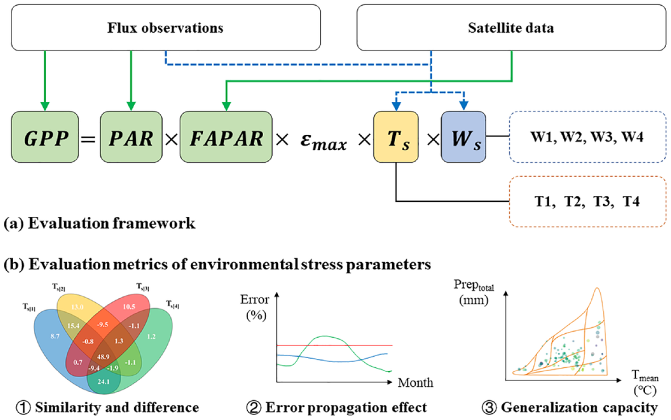
The LUE model framework for evaluating environmental stress parameters. (a) The structure of the common LUE model alongside the key environmental stress parameter in this study. (b) The aims of evaluation and corresponding metrics, which are described with more details in the evaluation method section.

Light use efficiency model

The light use efficiency model stands as a widely employed tool for estimating large-scale vegetation productivity, driven by remote sensing data and various environmental factors from multiple sources. The LUE model relies on two fundamental hypotheses: (1) the total primary productivity of the ecosystem is related to absorbed photosynthetically active radiation (APAR, which equals PAR×FAPAR); (2) the light use efficiency will be lower than its ideal value due to environmental stress, such as temperature stress or water stress. This concept can be expressed through the following equations:

\begin{matrix} G P P = P A R \times F A P A R \times ε \end{matrix}

(1)

\begin{matrix} G P P = P A R \times F A P A R \times (ε_{m a x} \times T_{s c a l a r} \times W_{s c a l a r} \times \dots) \end{matrix}

(2)

PAR is the incident photosynthetically active radiation (MJ/m²), FAPAR is the fraction of PAR absorbed by vegetation, ε is the actual light use efficiency (g C m² MJ⁻¹ APAR), ε_max is the maximum light use efficiency, T_s and W_s are the scalars to describe temperature stress and water stress, respectively.

We synthesized the main classic equations of temperature stress (T_s) and water stress (W_s) parameters. In this study, four types of temperature stress parameters and four types of water stress parameters were involved (Figure 2, Tables 1 and 2).

Figure 2.

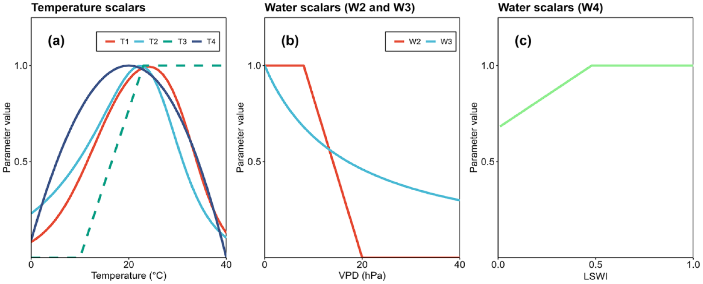
Partial stress functions of the light use efficiency models used in this study. (a) Temperature scalars, the solid line means the parameter is driven by mean temperatures, and the dashed line means the parameter is driven by minimum temperatures. (b) and (c) Water scalars, since the W1 parameter is driven by 2 variables, the 3D visible shape of W1 is relatively complex and not plotted in Figure 2 (but can be seen in Online Supplementary Figure S1). For the specific equations of those functions refer to Tables 1 and 2.

Table 1.

Equations of temperature related parameter in LUE models.

No.	Equation*	Model Name	References
T1	$T_{S} = T_{ε 1} \cdot T_{ε 2}$ $T_{ε 1} = 0.8 + 0.02 \cdot T_{o p t} - 0.0005 \cdot T_{o p t}^{2}$ $T_{ε 2} = 1.184 \cdot {(1 + e^{0.2 (T_{o p t} - 10 - T_{o b s})})}^{- 1} \cdot {(1 + e^{0.3 (- T_{o p t} - 10 + T_{o b s})})}^{- 1}$	CASA MuSyQ	(Potter et al., 1993)
T2	$p (T_{o b s}) = \frac{e^{(C_{1} - \frac{Δ H_{a . p}}{R_{g} T_{o b s}})}}{1 + e^{(\frac{Δ S T_{o b s} - Δ H_{d . p}}{R_{g} T_{o b s}})}}$	C-Fix	(Veroustraete et al., 2002; Wang, 1996)
T3	$T_{s} = \frac{T M I N_{o b s} - T M I N_{ε = 0}}{T M I N_{ε = m a x} - T M I N_{ε = 0}}$	MOD17 CFlux TL-LUE CI-LUE	(Running et al., 2004)
T4	$T_{s} = \frac{(T_{o b s} - T_{m i n}) (T_{o b s} - T_{m a x})}{[(T_{o b s} - T_{m i n}) (T_{o b s} - T_{m a x})] - {(T_{o b s} - T_{o p t})}^{2}}$	GLO-PEM EC-LUE VPM VPRM TEC	(Raich et al., 1991)

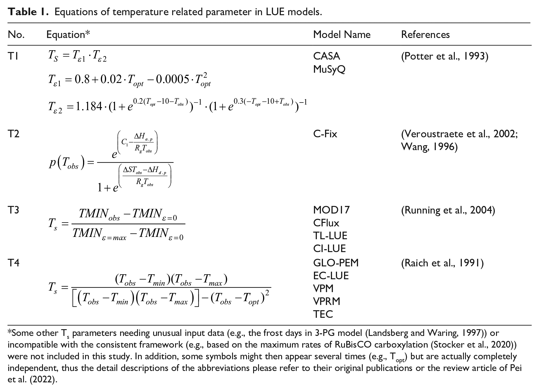
Some other T_s parameters needing unusual input data (e.g., the frost days in 3-PG model (Landsberg and Waring, 1997)) or incompatible with the consistent framework (e.g., based on the maximum rates of RuBisCO carboxylation (Stocker et al., 2020)) were not included in this study. In addition, some symbols might then appear several times (e.g., T_opt) but are actually completely independent, thus the detail descriptions of the abbreviations please refer to their original publications or the review article of Pei et al. (2022).

Table 2.

Equations of water related parameter in LUE models.

No.	Equation*	Model Name	References
W1	$W_{s} = \frac{L E}{L E + H}$	EC-LUE	(Yuan et al., 2007)
W2	$W_{s} = \frac{V P D_{ε = m a x} - V P D_{o b s}}{V P D_{ε = m a x} - V P D_{ε = 0}}$	MOD17 CFlux TL-LUE CI-LUE	(Running et al., 2004)
W3	$W_{s} = \frac{V P D_{0}}{V P D + V P D_{0}}$	Revised EC-LUE	(Yuan et al., 2019)
W4	$W_{s} = \frac{1 + L S W I}{1 + L S W I_{m a x}}$	VPM VPRM PCM MVPM	(Xiao et al., 2004)

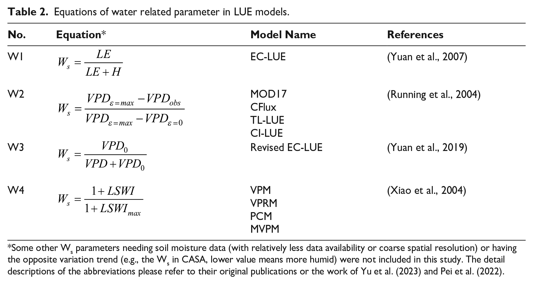
Some other W_s parameters needing soil moisture data (with relatively less data availability or coarse spatial resolution) or having the opposite variation trend (e.g., the W_s in CASA, lower value means more humid) were not included in this study. The detail descriptions of the abbreviations please refer to their original publications or the work of Yu et al. (2023) and Pei et al. (2022).

Data

Flux data

To quantify parameter differences across designs, the experiments were conducted by using the same dataset. The FLUXNET 2015 dataset (https://fluxnet.org/) was employed in this study to assess parameter performance. The total dataset comprises 212 flux observation sites, encompassing 13 vegetation types (with 182 sites located in northern hemisphere and 30 sites in southern hemisphere). To ensure the robustness in observation time and spatial representation, we specifically selected 147 sites (equivalent to 16,488 site-month data) with continuous observations spanning more than three years. This selection process ensured that each flux site had to contain a minimum of 36 site-month samples (refer to Online Supplementary Table S1 for the list of selected flux sites). The final set of sites encompasses 11 vegetation types (croplands, wetlands, grasslands, open shrublands, closed shrublands, savannas, woody savannas, deciduous broadleaf forests, mixed forests, evergreen broadleaf forests, evergreen needleleaf forests), with 128 sites located in the northern hemisphere and 19 sites in the southern hemisphere.

This study utilized GPP_NT_VUT_REF, mean/maximum/minimum daily temperatures, vapor pressure deficit (VPD), and latent/sensible heat flux data sourced from FLUXNET 2015. The flux GPP observation data serves as the benchmark for evaluation experiments. The observational data associated with temperature and moisture served as inputs for calculating environmental stress parameters in the LUE model framework (Figure 1).

Satellite data

Several parameters in the LUE models require satellite data as inputs. In this study, LSWI and NDVI data were specifically employed, in accordance with some equations governing W_s and T_s parameters. To facilitate the calculation of these remotely sensed indices (land surface water index (LSWI) and NDVI), the MCD43A4 V061 reflectance product was utilized. The MODIS MCD43A4 V061 is a Nadir Bidirectional Reflectance Distribution Function (BRDF)-Adjusted Reflectance (NBAR) dataset, which means the view angle effects are removed from the directional reflectance. This stable and consistent NBAR product ensures equitable cross-regional comparisons, enhancing the robustness of conclusions derived from site-scale experiments for regional or global applications. Meanwhile, the MOD15A2H V061 was employed as the source of FAPAR.

The satellite data for all flux sites were acquired from Google Earth Engine (GEE, https://earthengine.google.com/). For better match the footprint of flux observation, a sampling scale of 1000 meters was established for each flux site, and the corresponding satellite data for each site were extracted by using the area-weight resampling method. Given the MCD43A4 V061 is a daily dataset, we initially computed each remotely sensed index at the daily scale and subsequently aggregated it to the monthly scale by selecting the median value for each month. Similarly, since the MOD15A2H V061 is an 8-day dataset, we aggregated the FAPAR data to the monthly scale by selecting the median value for each month.

Evaluation methods

Commonality analysis

The commonality analysis (CA, also variance partitioning) is a tool to improves the ability to understand complex models through decomposing regression R² into unique and shared effects of independent variables, which is often visually depicted through Venn diagrams. Unique effects indicate the extent to which variance is exclusively accounted for by a single predictor, while shared effects demonstrate the portion of variance common to a set of predictors. Detailed calculations involved in variation partitioning have been well described elsewhere (Peres-Neto et al., 2006; Ray-Mukherjee et al., 2014).

In this study, we employed this tool to elucidate the similarities and differences among diverse parameters for temperature and water stress in LUE model, respectively. Specifically, we constructed several sub-models that exclusively involved parameters within one module (e.g., considering only the temperature stress parameters) for GPP estimation. Subsequently, we utilized the indicators of multicollinearity and shared variance to interpret intra-module similarities, while the unique variance was employed to signify intra-module differences among parameter designs. The values obtained from variance partitioning results indicate the respective capabilities to influence model estimations. In this study, higher values denote that a specific parameter design (e.g., the separate effect of T1) contributes more to GPP estimation. In other words, it also means taking the higher feature importance.

In our experiment, we utilized the R package rdacca.hp to perform the CA. It is a package that integrates related calculations (e.g., some methods in the vegan package) and can provide a significant level (whether a variable has significant effects on GPP estimation) based on the permutation test (Lai et al., 2022).

Error propagation analysis

The error propagation analysis was conducted through a simulation experiment. Since the inherent bias of input data for environmental stress parameters is that caused by scale effects or utilizations of proxy data, we make a random slight noise to simulate these kinds of errors and assess whether a slight difference of input data can lead to diverse effects on the final GPP estimations under different environmental stress function combinations. In theory, the extent of this effect depends on the specific equation of parameters and the seasonal variation of input environmental data. For instance, parameters expressed in linear form (e.g., the T_s in MOD17 model) would be relatively independent of the seasonal variation in input data. In contrast, parameters represented in parabolic or bell forms would be susceptible to fluctuations on days with relatively lower or higher factor values (e.g., days with temperature below 10°C).

In this study, we evaluated the error propagation effect by conducting simulation experiments based on real flux observations. Given the disparities in site numbers and seasonal variations, all flux sites were categorized into two groups in accordance with the northern and southern hemispheres. The LUE model was then executed to estimate GPP after introducing a 1.0% disturbance to the input data of environmental stress parameters (0.99 or 1.01 times to the original values). Consequently, this approach allowed us to evaluate both the individual error propagation effect (introducing noise to only one module, assuming only one input data has errors) and the joint error propagation effect (introducing noise to both temperature and water stress modules, assuming both input data have errors), which would match with the colorful application scenarios.

Generalization ability analysis

We combined the metrics derived from CA and several statistics about the GPP accuracy to evaluate the generalization ability of environmental stress parameters in LUE model. Given that the focus of this study is on environmental stress parameters rather than the entire LUE model, the generalization ability cannot be evaluated solely through cross-region GPP estimation accuracy (Yuan et al., 2014). Therefore, we analyzed the relationships between GPP and environmental stress parameters (T_s and W_s). More specifically, we used the GPP variability (the coefficient of variation in each site), GPP estimation accuracy metrics (R², rMAE and Residuals at each site) as indicators to evaluate the contribution level and the description ability of environmental stress parameters across a climate space. The contribution level is defined as the ratio between the variance of environmental stress parameters (both the total and separate variance) and the total R² of LUE model. For example, for a site with a low variance of T_s and W_s, it is suggested that the environmental stress parameters would have less ability to affect final estimations no matter how the environmental stress parameters change under its local environmental conditions. On the contrary, for a site with a high variance of T_s and W_s, it means the final GPP estimation is totally determined by environmental stress parameters rather than other factors (e.g., PAR and FAPAR). Meanwhile, the description ability is defined as the ratio of the coefficient of variation between GPP and environmental stress parameters, and the higher the value of this ratio the worse the ability of environmental stress parameters to describe GPP variations. After all, the variation of GPP is supposed to be larger than that of environmental stress parameters, since these parameters only describe one aspect of GPP. These metrics were computed for each flux site.

The climate space and linear regression methods were employed to yield qualitative and quantitative results, respectively. The relationship between GPP and environmental stress parameters would become evident when the statistics of each site are plotted in the climate space, with the x-axis representing mean annual temperature and the y-axis representing mean annual precipitation. For example, this approach allows for a clear visualization of the general pattern of the description ability of temperature stress parameters across different biomes within the climate space. Furthermore, given the monthly setting of the consistent LUE model framework, all flux data were aggregated into monthly averages for subsequent analyses. To address missing information on mean annual temperature and precipitation at certain sites, data from ERA5-land over the recent 30 years were utilized through the Google Earth Engine platform. Linear regression was employed to examine whether the contribution of environmental stress parameters correlates with GPP estimation accuracy.

Results

Intra-module parameters comparison

The performance of four temperature stress parameters in LUE model were generally homogenous yet differences also exist. The four types of T_s parameters shared 67.87 % variance for GPP estimation, which suggests they are generally homogenous or generally share similar physical meaning. In addition, the T1 parameters exerted the largest unique effect on GPP estimation (21.08% of total R²), whereas that of T2 and T3 parameters were relatively modest (below 1.0 %). Furthermore, these T_s parameters displayed moderate multicollinearity among themselves, as indicated by the Variance Inflation Factor (VIF) value (Figure 3). Specifically, the VIF of T3 and T4 parameters are above 10, which means their higher multicollinearity to the other T_s parameters. In addition, the T1 parameters showed the lowest VIF, indicating its relatively independent variation to the other T_s parameters. In short, based on the variance partitioning results, the T1 parameters and T4 parameters showed a relatively high capability in facilitating GPP estimation.

Figure 3.

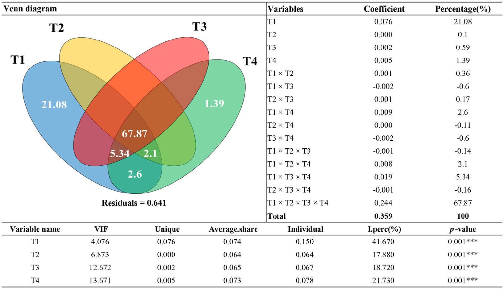
The result of commonality analysis for temperature stress parameters. The upper section displays a Venn diagram of such temperature stress parameters and the detail variance partitioning results. The lower section exhibits the corresponding statistics derived from the commonality analysis. VIF, variance inflation factor, an indicator for multicollinearity; Average.shared, total average shared effects with other predictors; I.prec, individual effect divided by total adjusted R² found in column Individual importance; p-values based on permutation test based on 999 randomizations and the values can vary from one run to another. For the specific equations of environmental stress functions refer to Tables 1 and 2. Notably, the part with a percentage below 1.0% was not annotated in Venn diagram. *** means p < 0.001.

The performance of four water stress parameters in LUE model exhibited significant differences. The CA results (Figure 4) revealed minimal variance shared among all four W_s parameters. Remarkably, the W1 parameter had the most substantial unique effect on GPP estimation, with the W3 and W4 parameters following. In addition, the unique effect of W2 parameter was marginal, suggesting that its information can be entirely represented by other parameters. Furthermore, the very low VIF value for these W_s parameters (all VIF values are below 5) also provide evidence of heterogeneity within the designs of moisture stress. In short, based on the variance partitioning results, both W1 parameters and W3 parameters showed a relatively high capability in facilitating GPP estimation.

Figure 4.

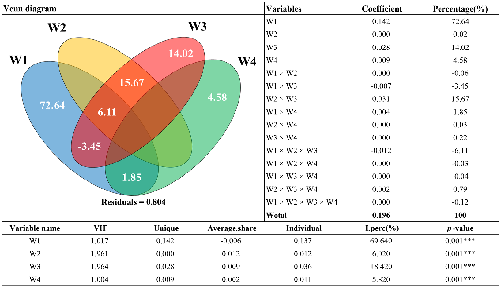
The result of commonality analysis for water stress parameters. The upper section displays the Venn diagram of such water stress parameters and the detail variance partitioning results. The lower section exhibits the corresponding statistics derived from the commonality analysis. VIF, variance inflation factor, an indicator for multicollinearity; Average.shared, total average shared effects with other predictors; I.prec, individual effect divided by total adjusted R² found in column Individual importance; p-values based on permutation test based on 999 randomizations, and the values can vary from one run to another. For the specific equations of environmental stress functions refer to Tables 1 and 2. Notably, the part with a percentage below 1.0% was not annotated in Venn diagram. *** means p < 0.001.

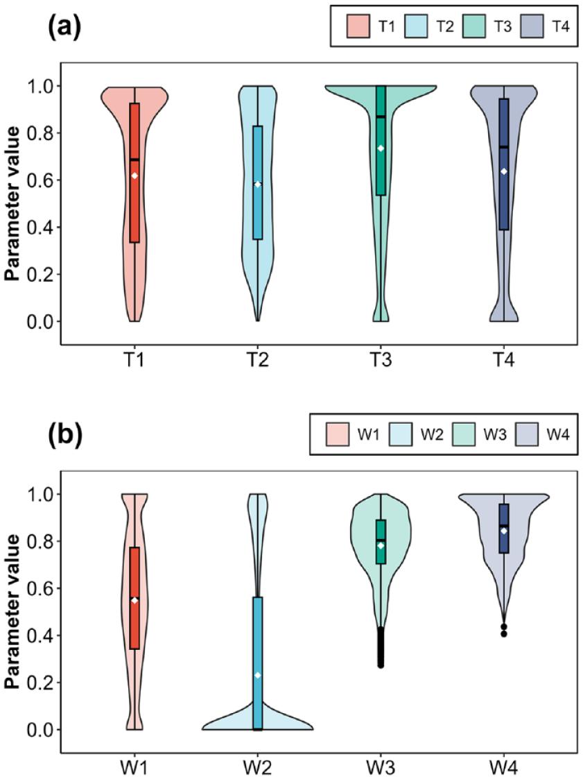
The intra-module differences were also reflected in the distribution of values. Despite the uniform value range of all T_s and water stress W_s parameters, spanning from 0 to 1, their value distributions exhibited notable diversity, particularly for the W_s parameters (Figure 5). For the T_s parameters, a higher concentration of calculation results was observed in the high-value range (with the exception of the T2 parameters), yet the extents of concentration were different from each other. In the case of W_s parameters, both W3 and W4 parameters had few samples located in the low-value range, while the W2 parameter exhibited a higher number of samples near zero.

Figure 5.

Distribution of value across environmental stress parameters. (a) The comparison of temperature stress parameters. (b) The comparison of water stress parameters. For the specific equations of environmental stress functions refer to Tables 1 and 2.

The error propagation effect of parameters

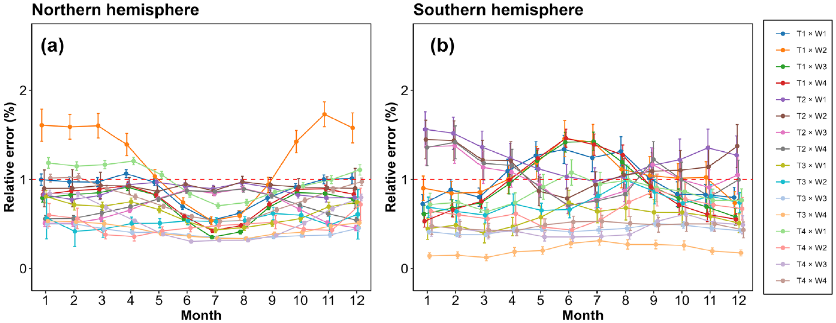
The error propagation effect from input data to final GPP estimations exhibited seasonal variability in both T_s and W_s parameters. The seasonal characteristics of the error propagation effect generally opposed each other between the northern and southern hemispheres, although this phenomenon was relatively less pronounced in the case of W_s parameters. Notably, the specific stress parameters with non-linear curve shapes, such as the T_s parameters in a bell shape (Figure 2), appeared to be more susceptible under situations with lower temperatures. For example, that depicted by the orange line in Figure 6a and c, its error propagation effect was higher during the corresponding winter period (e.g., June to August in the southern hemisphere) and even amplified the error beyond the level of additional artificial disturbance (1.0%).

Figure 6.

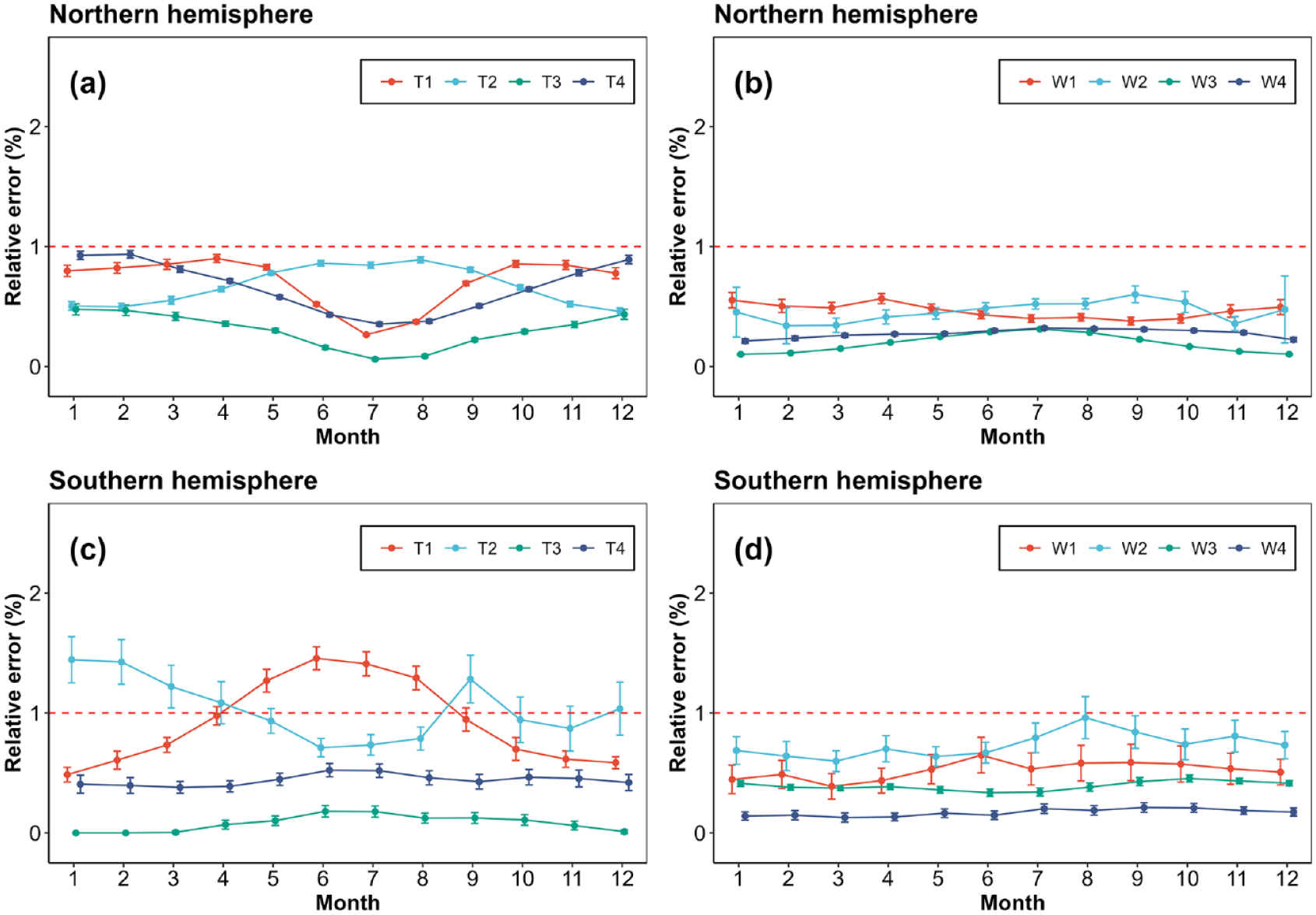
The seasonal variation of stress parameters’ separate error propagation effects in the LUE model. The error propagation effect of temperature stress parameters in (a) northern and (c) southern hemisphere. The error propagation effect of water stress parameters in (b) northern hemisphere and (d) southern hemisphere. For the specific equations of environmental stress functions refer to Tables 1 and 2.

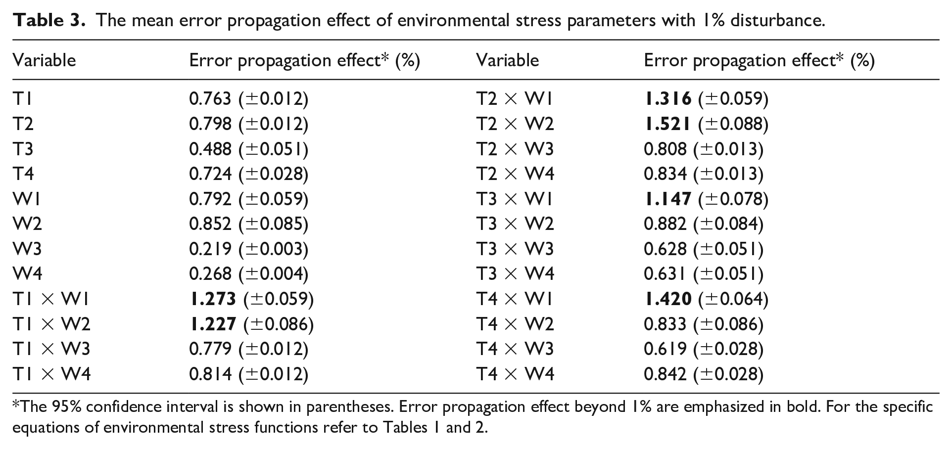
The error propagation effect would get larger when the input data for T_s and W_s parameters both contained the inherent bias. In actual applications, it is more common that both T_s and W_s parameters are driven by coarse grid data rather than flux or meteorological observations. According to the separate analysis of error propagation effect in T_s and W_s parameters, it is reasonable to assume some parameter combinations could reduce this kind of uncertainty, given the different seasonal characteristics of T_s and W_s parameters. However, the results showed that the joint error propagation effect tended to be larger (Table 3, Figure 7) than only considering single input data uncertainty (Figure 6). Specifically, certain combinations exhibited worse performance, resulting in relative errors exceeding the level of additional artificial disturbance (1.0%). Additionally, the seasonal variability of some combinations became more pronounced, with the difference between high and low values expanding (e.g., the dark orange line T1 × W2 in Figure 7a, compared with the orange line T1 in Figure 6a).

Table 3.

The mean error propagation effect of environmental stress parameters with 1% disturbance.

Variable	Error propagation effect* (%)	Variable	Error propagation effect* (%)
T1	0.763 (±0.012)	T2 × W1	1.316 (±0.059)
T2	0.798 (±0.012)	T2 × W2	1.521 (±0.088)
T3	0.488 (±0.051)	T2 × W3	0.808 (±0.013)
T4	0.724 (±0.028)	T2 × W4	0.834 (±0.013)
W1	0.792 (±0.059)	T3 × W1	1.147 (±0.078)
W2	0.852 (±0.085)	T3 × W2	0.882 (±0.084)
W3	0.219 (±0.003)	T3 × W3	0.628 (±0.051)
W4	0.268 (±0.004)	T3 × W4	0.631 (±0.051)
T1 × W1	1.273 (±0.059)	T4 × W1	1.420 (±0.064)
T1 × W2	1.227 (±0.086)	T4 × W2	0.833 (±0.086)
T1 × W3	0.779 (±0.012)	T4 × W3	0.619 (±0.028)
T1 × W4	0.814 (±0.012)	T4 × W4	0.842 (±0.028)

The 95% confidence interval is shown in parentheses. Error propagation effect beyond 1% are emphasized in bold. For the specific equations of environmental stress functions refer to Tables 1 and 2.

Figure 7.

The seasonal variation of stress parameters’ joint error propagation effects in the LUE model. The error propagation effect of temperature stress parameters in (a) northern and (b) southern hemisphere. The legend shows the 16 combinations of temperature and water stress parameters used in this study. For the specific equations of environmental stress functions refer to Tables 1 and 2.

The generalization capability of parameters

The effect of environmental stress parameters and the GPP estimation accuracy exhibited distinct patterns among the climate space. The total contribution of T_s + W_s, as derived from the CA, can elucidate the associations between environmental stress parameters and GPP estimation. This total contribution represented the combined variance of T_s and W_s parameters, which means the sum of V_shared (shared variance of T_s and W_s) and V_unique of T_s and W_s (unique variance of T_s and W_s, respectively). Its higher value signifies a greater influence of environmental stress parameters on GPP estimation. The results indicated that sites with better GPP estimation accuracy (higher R², lower rMAE) were predominantly situated in biomes characterized by moderate temperature and water conditions (Figure 8a and b), with environmental stress parameters contributing at a moderate level (green color). Conversely, sites within high temperatures, particularly those experiencing low water availability, exhibited diminished GPP estimation accuracy. Notably, the contribution of environmental stress parameters only had the high and low value in such areas, accompanied by concurrently high-level residuals (Figure 8d). In addition, the coefficient of variation of GPP is obviously larger than that of environmental stress parameters in regions with high temperatures, in comparison to other regions in the climate space (Figure 8c).

Figure 8.

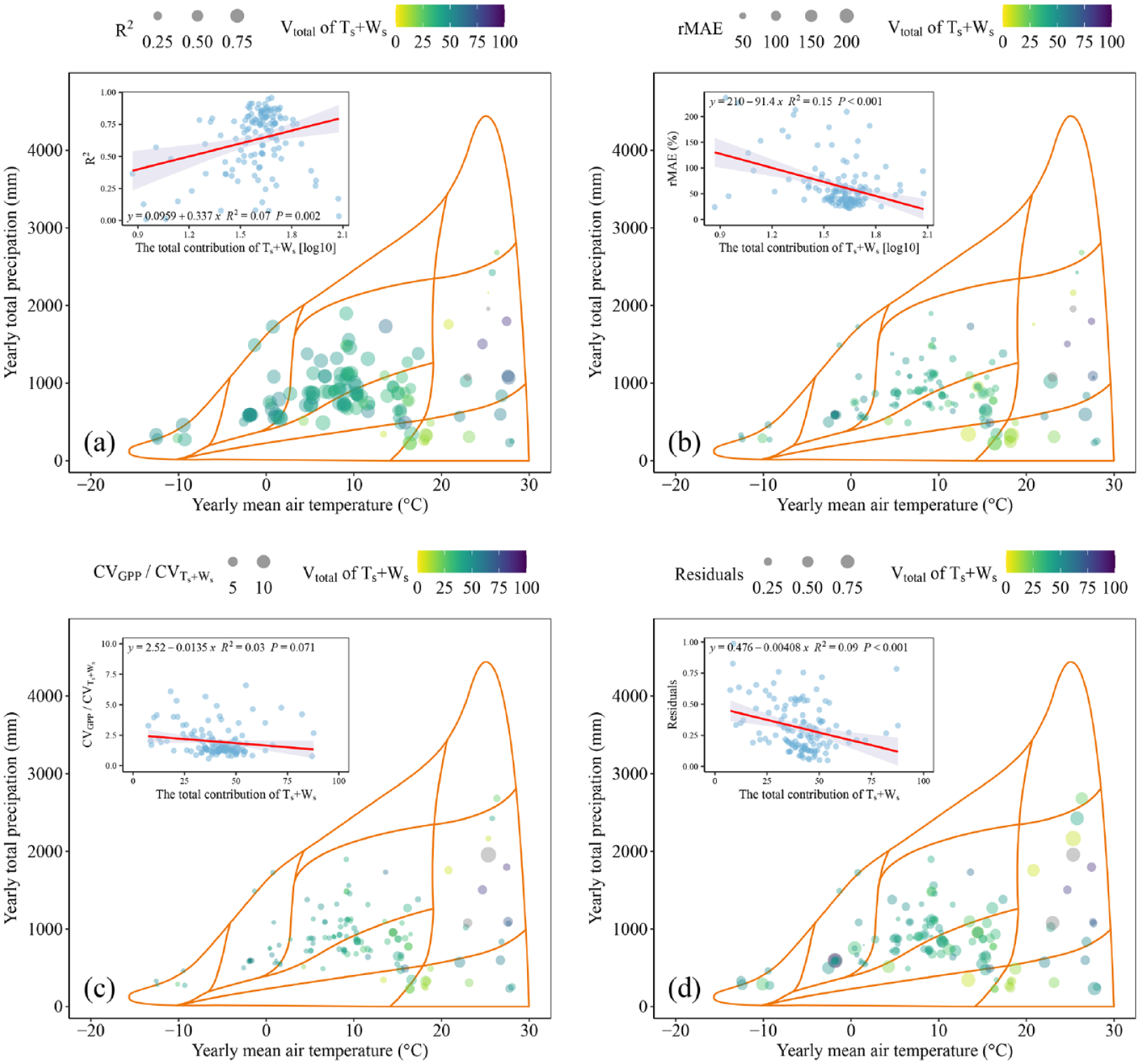
The relationship between evaluation metrics and environmental stress parameters. The total contribution of T_s + W_s (V_total of T_s + W_s) stands for the total variance ratio of T_s + W_s in LUE models (both the unique and shared), and it is shown as the points of color among all sub figures. Each point in the climate space stands for a flux site. The size of the points has different meaning in each sub figure: (a) the GPP estimation R² in each site; (b) the relative mean absolute error (MAE) in each site; (c) the ratio of CV_GPP to CV_{Ts + Ws} in each site; (d) the residuals of GPP estimation in each site. The polygons on the background shows the Whittaker’ biomes (see Online Supplementary Figure S2).

The description capability of environmental stress parameters varies across different regions. To assess this capability, we utilized the unique contributions of T_s and W_s derived from the CA (the coupled part of T_s and W_s were excluded), respectively. The ratio of the coefficient of variation of GPP (CV_GPP) to the CV of T_s/W_s was employed, with a high value indicating that GPP variability exceeds the description capacity of environmental stress parameters. The results revealed that regions with high temperatures exhibit a significant difference between the CV_GPP and the CV of T_s/W_s, particularly for temperature stress parameters (Figure 9b, where the CV_GPP is 10 times larger at some points). Additionally, in terms of the extent of unique contribution, the W_s parameters had relatively higher value which was larger than that of T_s (Figure 9), especially in the biomes with higher temperatures.

Figure 9.

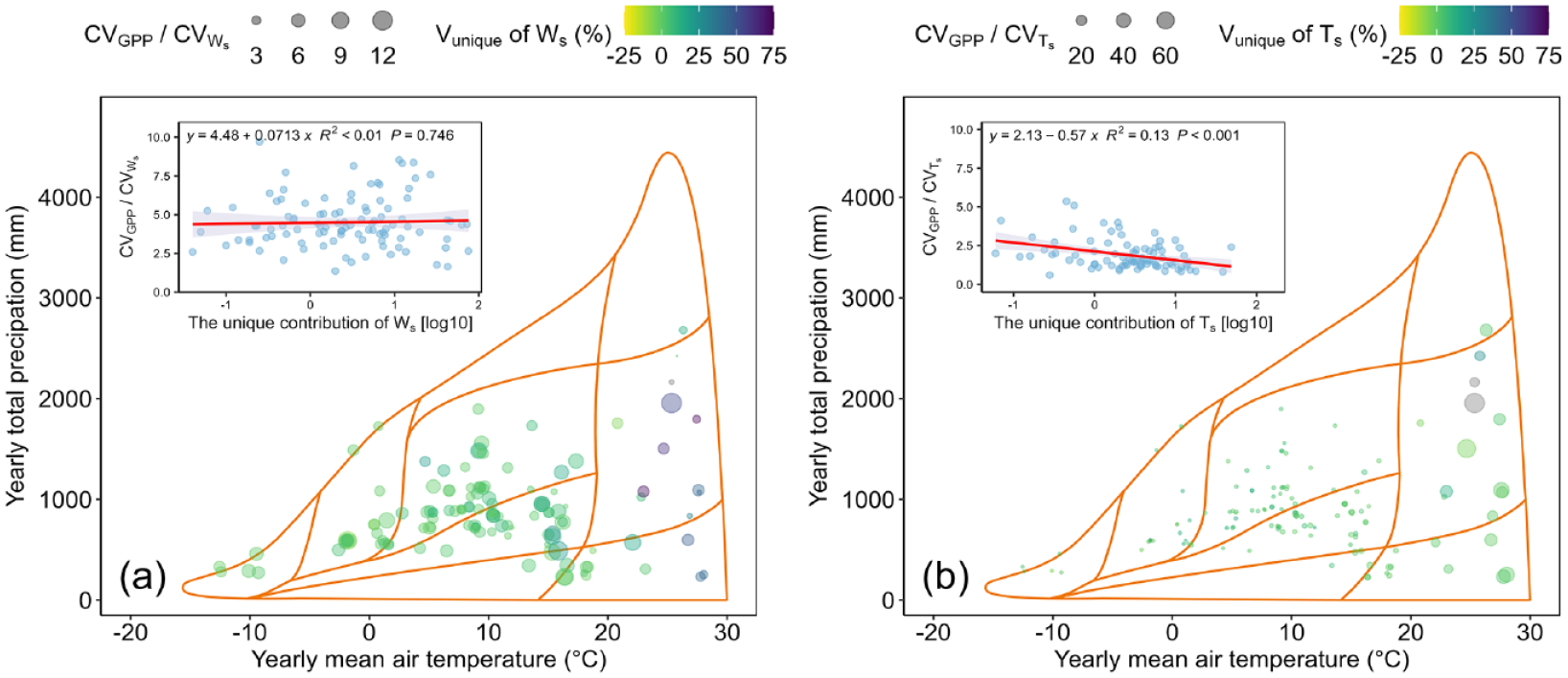
The description ability of temperature and stress parameters for GPP variability. Each point in the climate space stands for a flux site. The unique contribution of T_s and W_s stand for the unique variance ratio of T_s and W_s, respectively. The size of points has different meaning in each sub figure: (a) the ratio of CV_GPP to CV_Ts in each site; (b) the ratio of CV_GPP to CV_Ws in each site. The polygons on the background shows the Whittaker’ biomes (see Online Supplementary Figure S2).

Overall, the connection between the contribution of environmental stress parameters and estimation accuracy is evident, although this relationship is nonlinear. Meanwhile, environmental stress parameters exhibit diminished description capability in regions with relatively high temperatures, thereby compromising their universal generalization ability.

Discussion

The model uncertainties related to environmental stress parameters

Researchers tend pay more attention to screening the optimal parameter combination for GPP estimation, hence overlooking the uncertainties caused by distinct environmental stress parameter designs. Specifically, the current process of parameter selection lacks robustness, and the different conclusions of model performance evaluation are very much dependent on the specific dataset. For example, the VPM model exhibited varying performances in different studies, such as Zhang et al. (2017) (R² = 0.74, 113 sites) and Yuan et al. (2014) (R² = 0.44, 157 sites). Recently, Bao et al. (2022) synthesized six groups of environment stress functions in LUE models, not only involving temperature and water stress, and demonstrated that the optimal LUE model equations is largely different between the local and global scales. Although they discussed the reason why bell-shaped functions (e.g., the T1, used in CASA) in temperature stress description outperformed the sigmoid-like function (e.g., the T3, used in MOD17), the further differences within bell-shaped functions (e.g., the T1 and T4, used in CASA and VPM, respectively) were not fully discussed, except for its newly applied bell-shaped parameter considering the lagged effect (Horn and Schulz, 2011; Mäkelä et al., 2008). However, in this study, we revealed that the T1 and T4 parameters exhibit relatively higher unique effects on GPP estimation (Figure 3) and discussed their differences in value distributions (Figure 5) and performances in affecting error propagation (Figure 6). This finding also substantiated the superior performance of the bell-shaped temperature function compared to the sigmoidal function, which is consistent with the conclusion of Bao et al. (2022). Furthermore, our results highlighted that the T1 contributed the most unique variance among the four parameters considered in this study, and its lowest multicollinearity also proved that conclusion. In addition, our results support the partial rationality of flexibly combining the temperature stress parameter due to their general commonality, indicating they generally share the similar physical meaning (Figure 3). In contrast, water stress parameters appeared to exhibit less commonality (Figure 4), even though all of them follow a similar variation trend (low value means arid, high value means humid). In other words, these water stress parameters have distinct characteristics in physical meaning and value distributions, which is consistent with recent water constraints optimization research of the LUE model. Specifically, this research found that the estimation accuracy of LUE models can obviously be improved if the water related stress parameters are optimized. For example, the integrated water stress parameter derived from machine learning (Yu et al., 2023), the water stress parameters optimized for arid regions (Ding et al., 2024) and the design of applying both VPD- and soil water-related parameters (Bao et al., 2022; Stocker et al., 2020; Wang et al., 2018). These related studies also underscore the necessity and reliability to further improve the designs of environmental stress parameters.

The potential uncertainties associated with flexibly altering parameter combinations are often underestimated and manifest in two primary dimensions: (1) the parameter selection principle and (2) the amount of environmental stress parameters. In terms of the selection principle, numerous studies construct specific models by directly incorporating parameters from existing publications (Ding et al., 2024), which means a parameter combination may not have ever occurred in one structure before. Moreover, the rationale behind such combinations is underexplored, especially the potential physiological or mathematical implications. For the amount of parameters, some researchers combined the local knowledge and directly introduce multiple new environmental stress parameters alongside existing temperature and water stress parameters (Zhang et al., 2023). In other words, this approach assumes that the stress from diverse environmental factors are entirely independent, while certain studies adopt the minimum principle (only calculate the stress parameters with lowest value) for mitigation (Yuan et al., 2007). Although some studies demonstrated that applying two kinds of water stress parameters to describe water shortage and water availability concurrently can get a better performance in estimating GPP (Bagnara et al., 2015; Mäkelä et al., 2006; Stocker et al., 2020), our analysis of error propagation effect showed the potential uncertainty of increasing the number of environmental stress parameters without cautious considerations (Figure 7). In summary, an inappropriate combination of parameters in LUE models could magnify the inherent bias from input data.

In general, the uncertainties inherent in LUE models are contingent upon various factors (Pei et al., 2022), and the effect of intra-module designs should be emphasized. Although comparative experiments involving LUE models may yield disparate conclusions owing to differences in precondition settings, it is evident that environmental stress parameters exhibit divergences in their capabilities, emerging as substantial contributors to final estimation uncertainties. Meanwhile, the GPP estimation is a quantitative task that has high requirement on the accuracy of input data. However, the connections between the inherent bias of input data and the specific environmental stress parameter designs (or combinations) were less concurrently considered in LUE model construction. Therefore, the utilization and combination of environmental stress parameters in LUE model construction warrants a more cautious approach.

The proper environmental stress parameters for GPP estimation

Appropriate environmental stress parameters should contribute moderately to GPP estimation. The analysis of generalization ability revealed a nonlinear relationship between environmental stress parameters and estimation accuracy. Generally, as the total contribution of T_S + W_S increases, GPP estimation R² tends to rise, and rMAE tends to decrease. Notably, linear relationships emerge when transforming the total variance to the log scale (Figure 8a and b), suggesting a potential power function relationship wherein one unit contribution of environmental stress parameters would lead to a more substantial improvement in GPP estimation accuracy. However, the analysis of climate space indicates that excessively high or low contributions of T_S + W_S are also inappropriate, as observed in the lower right portion of Figure 8a and b (high temperature with low water conditions). For the actual designs of environmental stress parameters, the analysis results indicated that there should be fewer hard limitations in function designs (e.g., when observed VPD above 20hPa, the W_s parameter and whole GPP estimation would equal zero), since this kind of hard separation would completely determine final results and actually neglect the contribution of other parameters (e.g., PAR and FAPAR), which is also easily influenced from the inherent bias of input data.

The ability of existing environmental stress parameters cannot describe the GPP variation well in several biomes. It is reasonable to expect that the variation in GPP would be larger than that of each individual environmental stress parameter, given that these parameters only account for a specific aspect of GPP variability. Nevertheless, the disparities between them should not be too large. Otherwise, it indicates an insufficient description ability of the environmental stress parameter. In general, the result suggested that the description ability of environmental stress parameters performs well in most situations, except for regions with high temperatures (Figures 8c and 9), specifically in biomes such as tropical rain forest, tropical seasonal forest/savanna and subtropical desert. This outcome aligned with previous studies, highlighting persistently lower GPP estimations in evergreen broadleaf forests (Pei et al., 2022; Yuan et al., 2014) and the ongoing need for parameter optimization in arid and semi-arid regions (Ding et al., 2024; Yu et al., 2023). Furthermore, our results indicate that this difference in variations between GPP and environmental stress parameters is more pronounced in T_s parameters than in W_s parameters. Meanwhile, the higher unique effect tended to couple with lower difference in CV ratio (the significant linear trend in Figure 9b), although the trend appears less obvious in water stress parameters due to their lower commonality (large inter-parameter differences).

Overall, the current environmental stress parameters demonstrate acceptable performance across most situations, except for biomes with high temperatures. A higher contribution of environmental stress parameters to GPP tends to result in increased estimation accuracy. Efforts to minimize the variability gap between GPP and environmental stress parameters can enhance their contribution to GPP estimation. Notably, it is crucial to maintain a moderate contribution level for environmental stress parameters, considering the effect of PAR and FAPAR is also important. These characteristics can serve as guiding principles for the ongoing development of more suitable environmental stress parameters.

Limitations and prospects

While our experiments encompassed all flux sites with observations spanning over three years in FLUXNET 2015, it is challenging to assert that the quantity is entirely sufficient. The number of flux sites situated in the northern hemisphere significantly exceeds that in the southern hemisphere, resulting in a relatively larger error bar in statistical analyses (Figure 6c and d). Expanding the dataset to include more flux observations across diverse biomes, particularly sites situated in rainforests and subtropical deserts, would further implement the macro patterns between GPP estimation and environmental stress parameters in this study.

Given the strict demand for accurate quantitative estimation of GPP, there are still some uncertainties with the LUE model that need to be solved urgently, especially the difference between high R² and low rMAE (or rRMSE). In our study, the estimation R² for the example consistent framework were relatively high (range from 0.01 to 0.96 for each site, mean as 0.69 ± 0.04, Figure 8a left top). However, the rMAE were comparatively low (range from 21% to 200% for each site, mean as 56 ± 7%, Figure 8b left top). This phenomenon is recurrent in similar research, such as the optimal combination identified by Bao et al. (2022) (R² = 0.82, nRMSE = 40%). Our findings suggest that the lower description capability observed in several biomes may contribute to this uncertainty. Future investigations should prioritize biomes characterized by high R² and low rMAE to further elucidate this discrepancy.

Our study only considered the mainstream environmental stress parameters incorporated in widely adopted LUE models. Presently, numerous studies have developed an array of environmental stress parameters, including cloudiness index (Turner et al., 2006a; Wang et al., 2018) and clumping index (Zhang et al., 2023). Evaluating such diverse parameters within a consistent framework poses a challenge, particularly when simultaneously accounting for variations in the settings of FAPAR, PAR, and LUE_max. The future research needs to construct a more compatible framework to comprehensively evaluate these parameters, facilitating the development of parameters endowed with more realistic physical meaning.

Conclusions

This study systematically assessed the mainstream classic environmental stress parameters in light use efficiency GPP estimation model through a compatible framework. The evaluation focused on three key aspects: (1) identifying similarities and differences of environmental stress parameters; (2) evaluating the error propagation effect of input data under different environmental stress parameter combinations; and (3) assessing the generalization ability of environmental stress parameters. Our findings elucidated the factors influencing the superior performance of certain environmental stress parameters over others, and highlighted the potential uncertainties associated with current flexible parameter combinations in model construction. Furthermore, we further clarify the correlation between GPP estimation accuracy and environmental stress parameters, providing insights into the direction for improving parameter designs. The key conclusions are summarized as follows:

(1) The four classic temperature stress parameters exhibit overall homogeneity (shared 67.87% variance), while the four classic water stress parameters demonstrate noticeable internal disparities (shared variance below 1.0%).

(2) Current flexible parameter combination method in LUE model construction should be more cautious, since it can amplify the inherent bias of input data. Some certain combinations of environmental stress parameters can generally maintain the extent of error propagation effect from the inherent bias of input data.

(3) The performance of current classic environmental stress parameters in the LUE model is generally acceptable, yet they perform less well in the biomes with high temperatures. In addition, the variance of environmental stress parameters was coupled to the estimation accuracy of LUE model, and the ability to describe GPP variation is positively related to the unique variance of environmental stress parameters (especially for T_s parameters).

Supplemental Material

sj-docx-1-tee-10.1177_2754124X241235545 – Supplemental material for Uncertainty analysis of intra-module environmental stress parameter design in light use efficiency-based gross primary productivity estimation models

Supplemental material, sj-docx-1-tee-10.1177_2754124X241235545 for Uncertainty analysis of intra-module environmental stress parameter design in light use efficiency-based gross primary productivity estimation models by Cenliang Zhao and Wenquan Zhu in Transactions in Earth, Environment, and Sustainability

Footnotes

Code and data availability

The processed data for each site and corresponding codes are available on author Cenliang Zhao’s GitHub website ().

Declaration of conflicting interests

The author(s) declared no potential conflicts of interest with respect to the research, authorship, and/or publication of this article.

Funding

The author(s) disclosed receipt of the following financial support for the research, authorship, and/or publication of this article: This study is financially supported by the National Key Research and Development Program of China (Grant No. 2020YFA0608504) and the Second Tibetan Plateau Scientific Expedition and Research Program (STEP) (Grant No. 2019QZKK0606). We appreciate FLUXNET () and MODIS for their open-source data services.

ORCID iDs

Cenliang Zhao

Wenquan Zhu

Supplemental Material

Supplemental material for this article is available online.

Author biographies

Cenliang Zhao is currently working toward the Ph.D. degree in cartography and geography information system with Beijing Normal University, Beijing, China. He received the B.Sc. degree in resources and environmental science from Faculty of Geographical Science, Beijing Normal University, Beijing, China, in 2019. His research interests include ecological remote sensing and digital image processing.

Wenquan Zhu is currently a professor in Beijing Normal University. He received the M.Sc. degree in ecology from Institute of Applied Ecology, Chinese Academy of Sciences, Shenyang, China, in 2002 and the Ph.D. degree in cartography and geography information system from Beijing Normal University, Beijing, China, in 2005. His research interests include remote sensing image processing, analysis, and application in land-cover/land-use change and vegetation dynamics.

References

Badgley

Anderegg

LDL

Berry

, et al (2019) Terrestrial gross primary production: Using NIRV to scale from site to globe. Global Change Biology 25: 3731–3740.

Bagnara

Sottocornola

Cescatti

, et al (2015) Bayesian optimization of a light use efficiency model for the estimation of daily gross primary productivity in a range of Italian forest ecosystems. Ecological Modelling 306: 57–66.

Bao

Wutzler

Koirala

, et al (2022) Environment-sensitivity functions for gross primary productivity in light use efficiency models. Agricultural and Forest Meteorology 312: 108708.

Ding

, et al (2024) A water stress factor based on normalized difference water index substantially improved the accuracy of light use efficiency model for arid and semi-arid grasslands. Journal of Environmental Management 349: 119566.

Frouin

Pinker

(1995) Estimating Photosynthetically Active Radiation (PAR) at the earth’s surface from satellite observations. Remote Sensing of Environment 51: 98–107.

Gonsamo

Chen

(2018) Vegetation primary productivity. In: Liang

(ed.) Comprehensive Remote Sensing. Oxford: Elsevier, 163–189.

Zhou

, et al (2013) Development of a two-leaf light use efficiency model for improving the calculation of terrestrial gross primary productivity. Agricultural and Forest Meteorology 173: 28–39.

Kimball

Running

, et al (2016) Satellite detection of soil moisture related water stress impacts on ecosystem productivity using the MODIS-based photochemical reflectance index. Remote Sensing of Environment 186: 173–183.

Horn

Schulz

(2011) Identification of a general light use efficiency model for gross primary production. Biogeosciences 8: 999–1021.

10.

Jiang

Ryu

(2016) Multi-scale evaluation of global gross primary productivity and evapotranspiration products derived from Breathing Earth System Simulator (BESS). Remote Sensing of Environment 186: 528–547.

11.

Lai

Zou

Zhang

, et al (2022) Generalizing hierarchical and variation partitioning in multiple regression and canonical analyses using the rdacca.hp R package. Methods in Ecology and Evolution 13: 782–788.

12.

Landsberg

Waring

(1997) A generalised model of forest productivity using simplified concepts of radiation-use efficiency, carbon balance and partitioning. Forest Ecology and Management 95: 209–228.

13.

Lin

Chen

, et al (2017) Seasonal fluctuations of photosynthetic parameters for light use efficiency models and the impacts on gross primary production estimation. Agricultural and Forest Meteorology 236: 22–35.

14.

Huete

, et al (2014) Parameterization of an ecosystem light-use-efficiency model for predicting savanna GPP using MODIS EVI. Remote Sensing of Environment 154: 253–271.

15.

Mahadevan

Wofsy

Matross

, et al (2008) A satellite-based biosphere parameterization for net ecosystem CO₂ exchange: Vegetation Photosynthesis and Respiration Model (VPRM). Global Biogeochemical Cycles 22(2): 10.1029/2006GB002735.

16.

Mäkelä

Kolari

Karimäki

, et al (2006) Modelling five years of weather-driven variation of GPP in a boreal forest. Agricultural and Forest Meteorology 139: 382–398.

17.

Mäkelä

Pulkkinen

Kolari

, et al (2008) Developing an empirical model of stand GPP with the LUE approach: Analysis of eddy covariance data at five contrasting conifer sites in Europe. Global Change Biology 14: 92–108.

18.

Myneni

Hoffman

Knyazikhin

, et al (2002) Global products of vegetation leaf area and fraction absorbed PAR from year one of MODIS data. Remote Sensing of Environment 83: 214–231.

19.

Pei

Dong

Zhang

, et al (2022) Evolution of light use efficiency models: Improvement, uncertainties, and implications. Agricultural and Forest Meteorology 317: 108905.

20.

Peres-Neto

Legendre

Dray

, et al (2006) Variation partitioning of species data matrices: Estimation and comparison of fractions. Ecology 87: 2614–2625.

21.

Piao

Wang

Park

, et al (2020) Characteristics, drivers and feedbacks of global greening. Nature Reviews Earth & Environment 1: 14–27.

22.

Potter

Randerson

Field

, et al (1993) Terrestrial ecosystem production: A process model based on global satellite and surface data. Global Biogeochemical Cycles 7: 811–841.

23.

Prince

Goward

(1995) Global primary production: A remote sensing approach. Journal of Biogeography 22: 815–835.

24.

Raich

Rastetter

Melillo

, et al (1991) Potential net primary productivity in South America: Application of a global model. Ecological Applications 1: 399–429.

25.

Ray-Mukherjee

Nimon

Mukherjee

, et al (2014) Using commonality analysis in multiple regressions: A tool to decompose regression effects in the face of multicollinearity. Methods in Ecology and Evolution 5: 320–328.

26.

Running

Nemani

Heinsch

, et al (2004) A continuous satellite-derived measure of global terrestrial primary production. BioScience 54: 547–560.

27.

Running

Thornton

Nemani

, et al (2000) Global terrestrial gross and net primary productivity from the earth observing system. In: Sala

Jackson

Mooney

, et al (eds) Methods in Ecosystem Science. New York, NY: Springer, 44–57.

28.

Ryu

Jiang

Kobayashi

, et al (2018) MODIS-derived global land products of shortwave radiation and diffuse and total photosynthetically active radiation at 5km resolution from 2000. Remote Sensing of Environment 204: 812–825.

29.

Stocker

Wang

Smith

, et al (2020) P-model v1.0: An optimality-based light use efficiency model for simulating ecosystem gross primary production. Geoscientific Model Development 13: 1545–1581.

30.

Tramontana

Jung

Schwalm

, et al (2016) Predicting carbon dioxide and energy fluxes across global FLUXNET sites with regression algorithms. Biogeosciences 13: 4291–4313.

31.

Turner

Ritts

Cohen

, et al (2006a) Evaluation of MODIS NPP and GPP products across multiple biomes. Remote Sensing of Environment 102: 282–292.

32.

Turner

Ritts

Styles

, et al (2006b) A diagnostic carbon flux model to monitor the effects of disturbance and interannual variation in climate on regional NEP. Tellus B: Chemical and Physical Meteorology 58: 476–490.

33.

Veroustraete

Sabbe

Eerens

(2002) Estimation of carbon mass fluxes over Europe using the C-Fix model and Euroflux data. Remote Sensing of Environment 83: 376–399.

34.

Wang

K-Y

(1996) Canopy CO2 exchange of Scots pine and its seasonal variation after four-year exposure to elevated CO2 and temperature. Agricultural and Forest Meteorology 82: 1–27.

35.

Wang

Huang

Yan

, et al (2015) Improving the light use efficiency model for simulating terrestrial vegetation gross primary production by the inclusion of diffuse radiation across ecosystems in China. Ecological Complexity 23: 1–13.

36.

Wang

Ibrom

Bauer-Gottwein

, et al (2018) Incorporating diffuse radiation into a light use efficiency and evapotranspiration model: An 11-year study in a high latitude deciduous forest. Agricultural and Forest Meteorology 248: 479–493.

37.

Xiao

Hollinger

Aber

, et al (2004) Satellite-based modeling of gross primary production in an evergreen needleleaf forest. Remote Sensing of Environment 89: 519–534.

38.

Xiao

Liang

Sun

(2018) Evaluation of three long time series for global Fraction of Absorbed Photosynthetically Active Radiation (FAPAR) products. IEEE Transactions on Geoscience and Remote Sensing 56: 5509–5524.

39.

Xie

Zhao

Zhu

, et al (2023) A radiation-regulated dynamic maximum light use efficiency for improving gross primary productivity estimation. Remote Sensing 15: 1176.

40.

Yao

Tang

, et al (2023) Coupling a light use efficiency model with a machine learning-based water constraint for predicting grassland gross primary production. Agricultural and Forest Meteorology 341: 109634.

41.

Yuan

Cai

Xia

, et al (2014) Global comparison of light use efficiency models for simulating terrestrial vegetation gross primary production based on the LaThuile database. Agricultural and Forest Meteorology 192/193: 108–120.

42.

Yuan

Liu

, et al (2010) Global estimates of evapotranspiration and gross primary production based on MODIS and global meteorology data. Remote Sensing of Environment 114: 1416–1431.

43.

Yuan

Liu

Zhou

, et al (2007) Deriving a light use efficiency model from eddy covariance flux data for predicting daily gross primary production across biomes. Agricultural and Forest Meteorology 143: 189–207.

44.

Yuan

Zheng

Piao

, et al (2019) Increased atmospheric vapor pressure deficit reduces global vegetation growth. Science Advances 5: eaax1396.

45.

Zhang

Bai

Sun

, et al (2023) An improved light use efficiency model by considering canopy nitrogen concentrations and multiple environmental factors. Agricultural and Forest Meteorology 332: 109359.

46.

Zhang

Liang

Zhou

, et al (2014) Generating Global LAnd Surface Satellite incident shortwave radiation and photosynthetically active radiation products from multiple satellite data. Remote Sensing of Environment 152: 318–332.

47.

Zhang

Xiao

, et al (2017) A global moderate resolution dataset of gross primary production of vegetation for 2000–2016. Scientific Data 4: 170165.

48.

Zhao

Zhu

Xie

(2024) Comparative evaluation of simulation methods for vegetation maximum light use efficiency. National Remote Sensing Bulletin 28(3). DOI: 10.11834/jrs.20211394.

49.

Zheng

Shen

Wang

, et al (2020) Improved estimate of global gross primary production for reproducing its long-term variation, 1982–2017. Earth System Science Data 12: 2725–2746.

Supplementary Material

Please find the following supplemental material available below.

For Open Access articles published under a Creative Commons License, all supplemental material carries the same license as the article it is associated with.

For non-Open Access articles published, all supplemental material carries a non-exclusive license, and permission requests for re-use of supplemental material or any part of supplemental material shall be sent directly to the copyright owner as specified in the copyright notice associated with the article.

0.00 MB

0.15 MB