Sage Journals: Discover world-class research

Abstract

The health risks associated with particulate matter pollution (PM_2.5) highlight the importance of comprehending key drivers of its spatial and temporal variability. While explanatory modeling is widely used for statistical inference in such applications, the role of wind variables (speed, direction) and their interplay with built environment are often overlooked. This study addresses this gap through a mobile air quality campaign in a suburban area over 10 days for each of three distinct seasons. We developed four innovative wind-based buffers to account for the wind factors and assess the impact of LiDAR-derived 3D built environment structure on PM_2.5 variability at local and regional scales. Our second objective is to assess the predictive capabilities of wind-based variables. Results indicate that in our low-elevation, low-rise building study area, the built environment does not emerge as a significant factor, contrary to findings in larger, denser urban areas. Wind direction proves more effective in capturing concentration fluctuations than wind speed, and its interaction with pollution source orientation can change pollution dynamics. This study introduces new insights and methodologies for incorporating wind-related factors into the analysis of air pollution dynamics, offering opportunities for further investigation in various urban settings.

Keywords

particulate pollution wind-based buffers mobile monitoring GIS LiDAR

Introduction

Outdoor air pollution is a significant threat to human health, contributing to approximately 4.2 million premature deaths worldwide each year (WHO, 2018). It ranks fifth among the leading causes of mortality globally (Cohen et al., 2017). Fine particulate matter or PM_2.5 exhibits a high lethality because of its ability to quickly penetrate a person’s bloodstream and organs following inhalation (Chowdhury et al., 2016). Even at low concentrations, PM_2.5 has a significant impact on life expectancy (Vodonos et al., 2018), giving rise to a range of health issues (Cao et al., 2018). PM_2.5 is commonly emitted from various sources such as industry, automobile and diesel exhaust, and street-level activities like cooking or construction (Ariunsaikhan et al., 2020).

Conventionally, long-term PM_2.5 monitoring is typically conducted by government-regulated air monitoring stations. However, many U.S. cities only have one PM_2.5 regulatory instrument to represent city-wide concentrations (Bi et al., 2020), potentially leading to spatially biased health-effect estimates (Hu et al., 2017). Notably, street-level PM_2.5 concentrations exhibit high variability (Li et al., 2018; Liang et al., 2023; Snyder et al., 2013), due to their sensitivity to various factors, including climatic conditions (Miao et al., 2020; Zhang et al., 2018), landscape features (Hu et al., 2021; Song et al., 2022; Tian et al., 2019), traffic volumes (Charron et al., 2005; Park et al., 2021), and greenspace (Abhijith et al., 2017). Mobile monitoring using low-cost sensors (LCS) on transportation modes such as bicycles, buses, or walkers is gaining popularity for its ability to identify PM_2.5 hotspots and detect street-level spatial-temporal variations efficiently (Fruin et al., 2008; Tong et al., 2021).

Despite the widespread adoption of mobile monitoring in urban science, several shortcomings exist in the current studies. Firstly, while there is previous evidence of seasonal changes in PM_2.5 (Li et al., 2016; Mi et al., 2019; Miao et al., 2020), many mobile monitoring studies are often limited to a single season or a low sampling frequency (Ke et al., 2022; Qiu et al., 2019; Zhou and Lin, 2019). Past studies also tend to limit mobile sampling to 10 runs or less, which may not adequately capture intra-urban PM_2.5 changes (Van Poppel et al., 2013). Secondly, in street-level PM_2.5 concentration prediction, horizontal urban structure features like patch density, shape index, and connectance index are commonly addressed (Dadvand et al., 2015; Ke et al., 2022). However, the impacts of vertical urban structure features, which relate to the height and volume of urban canopy, are often overlooked (Ke et al., 2022; Miskell et al., 2015; Xu and Chen, 2021). Thirdly, the assessment of the influence of regional landscape on PM_2.5 often relies on circular buffers, assuming a homogenous wind direction and source location (Gilliland et al., 2018; Meng et al., 2015; Naughton et al., 2018; Tian et al., 2019). Some studies employed semicircular vectors that focus on changes in prevailing wind direction, considering upwind and downwind dynamics only (Li et al., 2015), while others investigated detailed wind-related changes but omitted the consideration of scale (Hart et al., 2020). While diverse wind patterns can interact with street geometries in various ways (Chatzidimitriou and Yannas, 2017; Huang et al., 2019; Karra et al., 2017; Wang et al., 2022), it is important to assess the effectiveness of incorporating both wind speed and direction in understanding PM_2.5 variation. Lastly, most studies use statistical models on a macro-scale that span multiple cities or nationwide (She et al., 2017; Weissert et al., 2019; Yuan et al., 2019; Zhang et al., 2022). However, it is worth noting that PM_2.5 relationships with micro-scale conditions can differ from those observed at meso- or macro-scales (Alzuhairi et al., 2016; Kim et al., 2015; Wang et al., 2022).

To address the above research gaps, our study has two primary objectives. The first objective is to explore various wind-based buffer computation methods of measuring 3D morphologies at both micro and meso scale. The second objective is to explore how wind speed and wind direction affect PM_2.5 concentration. We aimed to determine if adding wind-based variables improves modeling capability compared to just including basic wind parameters.

Study area

In contrast to previous studies that have primarily focused on K-12 educations settings (Erlandson et al., 2019), this study was conducted at the University of North Texas (UNT) campus. UNT is situated in the city of Denton in the northern region of the Dallas-Fort Worth-Arlington Metroplex (DFW). Even though Denton is not classified as a non-attainment area for particulate pollution, the rapid pace of urbanization in recent decades has sparked concerns about deteriorating air quality. As of 2020, Denton has a sizeable population of 147,825, marking a 30.7% growth since 2010. Projections indicate that the population is expected to reach 207,334 by 2030 (City of Denton, 2022; Tsiaperas, 2022; U.S. Census Bureau, 2022). Notably, Denton is uniquely located at the convergence of Interstate 35E and 35W, which serve as major highways connecting various cities in the region. Despite all the intensified human activities, the only regulatory air quality station in Denton County is in a suburban-rural transitional zone that is approximately four km away from UNT. The main UNT campus covers an area of approximately one km², with many low-rise buildings and a mix of juvenile and fully grown trees (Figure 1). The average building height for the campus is 11 meters with a standard deviation of 7.13 meters. The maximum building height is 41 meters. With over 42,000 students, UNT experiences ongoing active construction activities (UNT News Service, 2022). Moreover, air quality at UNT is adversely affected by vehicular emissions from heavy-duty diesel vehicles on the nearby major Interstate-35 (I-35) and industrial emissions from cement plants in the southern DFW region (Bryant, 2021).

Figure 1.

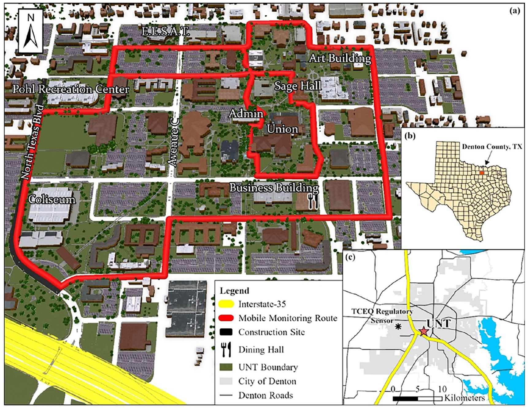
Map of study area. (a) The mobile monitoring route overlaid on the University of North Texas (UNT) virtual campus; (b) Denton County in the state of Texas, USA; (c) UNT Campus in Denton, TX, with the only Texas Commission of Environmental Quality (TCEQ) station that includes a PM_2.5 regulatory instrument in the west.

Methods

Two sets of models were developed to address the two objectives (Figure 2). For Objective 1, we developed and assessed eight multi-scale wind-based buffer methods for calculating street-level 3D urban built environment. For Objective 2, we constructed seven ordinary least squares (OLS) regression models based on wind parameters and buffer-derived vertical morphological variables, to understand the significance of other wind-related variables in the dynamics of air pollution.

Figure 2.

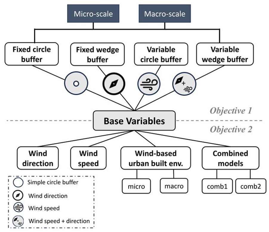
Flowchart depicting the workflows for Objectives 1 and 2.

Mobile monitoring campaign

Field sampling and data collection

Multiple mobile monitoring campaigns were conducted over three seasons, specifically from April 25 to May 6, 2022 (Spring), July 4 to July 15, 2022 (Summer), and September 26 to October 7, 2022 (Fall). During these campaigns, a battery-operated Dylos DC1700 laser particle counter was used to record PM_2.5 particle concentrations (ug/m³) at 1-minute intervals. This resolution was recommended as suitable for representing fine scale PM_2.5 variations (Li et al., 2018). A Montana 650t GPS unit was used to record GPS tracks at a rate of approximately 5–10 GPS points per minute. Trained volunteer bikers followed data collection protocol described in Hart et al., 2020, traversing a predetermined 1.6-mile route with the two devices (Figure S1). Sampling was conducted on weekdays at specific hours to capture diurnal variation, including peak commute periods at UNT (7 AM and 3 PM) and times of low campus traffic (11 AM and 7 PM). Each sampling session took approximately 30 minutes and was conducted on consecutive weekdays for two weeks per season. A total of 160 hourly samples were collected, with each season represented by 40 samples.

Data preprocessing

Since the Dylos sensor and GPS unit collect data at different frequency, GPS coordinates falling within each 1-minute timestamp of PM_2.5 points were consolidated to align the data. To analyze repeated measurement along the same road across seasons and address minor inaccuracies in GPS points, we assigned each PM_2.5 measurement to the nearest 100-meter road segment using a “snapping” procedure (Apte et al., 2017; Messier et al., 2018). We chose 100 m by considering the spatial resolution and sample size (Kerckhoffs et al., 2016; Li et al., 2016; Shi et al., 2019). To mitigate the effect of extreme outliers of PM_2.5 values, median values were calculated for each route segment (Li et al., 2018).

Explanatory variables

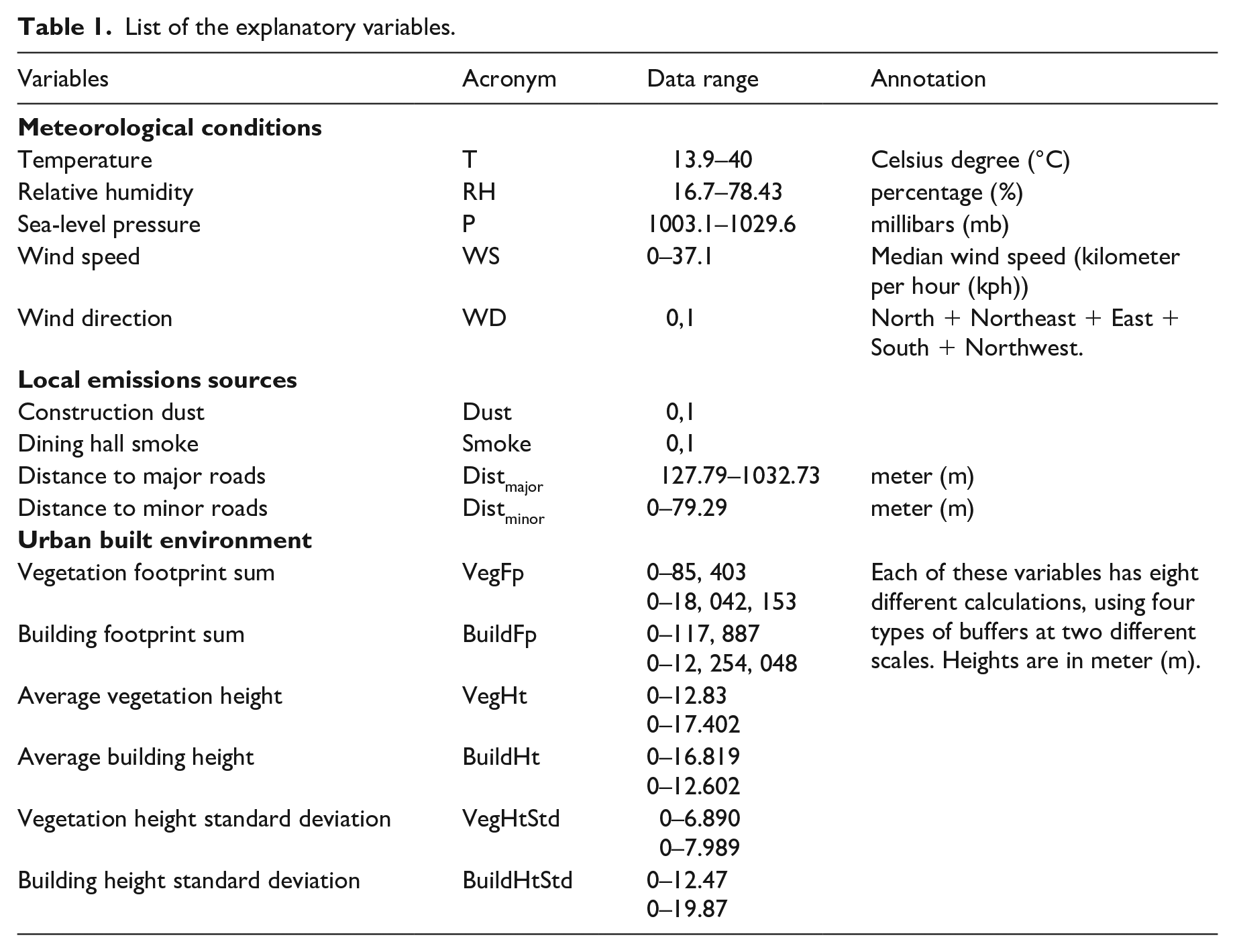
Table 1 lists a set of explanatory variables used in this study, including meteorological, wind-related, local hotspot and emission variables, and 3D urban morphological indicators.

Table 1.

List of the explanatory variables.

Variables	Acronym	Data range	Annotation
Meteorological conditions
Temperature	T	13.9–40	Celsius degree (°C)
Relative humidity	RH	16.7–78.43	percentage (%)
Sea-level pressure	P	1003.1–1029.6	millibars (mb)
Wind speed	WS	0–37.1	Median wind speed (kilometer per hour (kph))
Wind direction	WD	0,1	North + Northeast + East + South + Northwest.
Local emissions sources
Construction dust	Dust	0,1
Dining hall smoke	Smoke	0,1
Distance to major roads	Dist_major	127.79–1032.73	meter (m)
Distance to minor roads	Dist_minor	0–79.29	meter (m)
Urban built environment
Vegetation footprint sum	VegFp	0–85, 4030–18, 042, 153	Each of these variables has eight different calculations, using four types of buffers at two different scales. Heights are in meter (m).
Building footprint sum	BuildFp	0–117, 8870–12, 254, 048
Average vegetation height	VegHt	0–12.830–17.402
Average building height	BuildHt	0–16.8190–12.602
Vegetation height standard deviation	VegHtStd	0–6.8900–7.989
Building height standard deviation	BuildHtStd	0–12.470–19.87

Meteorological variables

To assess the seasonal influence on PM_2.5 variation (Miao et al., 2020), weather data including hourly temperature (°C), relative humidity (%), wind direction (degrees), wind gust (km/h), and wind speed (km/h) were obtained from the nearby TCEQ Denton station (access through NOAA National Centers for Environmental Information, 2022). For each season, the relevant variables were extracted and joined with geolocated PM_2.5 concentrations to the nearest hour. To test the seasonality effect, spring, fall, and summer were included as three indicator variables, with summer serving as the reference category to assess significance between warm and cool seasons. Wind direction was categorized into eight sectors: N (−22.5 to 22.5°), NE (22.5 to 67.5°), E (67.5 to 112.5°), SE (112.5 to 157.5°), S (157.5 to 202.5°), SW (202.5 to 247.5°), W (247.5 to 292.5°), and NW (292.5 to 337.5°). Each sector was represented by a binary variable, with a value of 1 indicating the presence of the corresponding wind direction for a given time snap. Southeast, the prevailing wind direction, served as the reference category, enabling us to evaluate the statistical significance of different wind directions on PM_2.5 levels. Due to a limited sample size, westerly and southwesterly winds were excluded from the model.

Proximity to traffic

Previous studies have observed a distance decay of PM_2.5 with proximity to roads (Gilliland et al., 2018; Liu et al., 2020). To assess this effect, we acquired the road network data from Denton County GIS hub (Denton County, 2022) and categorized the roads into major and minor types. We also manually geolocated the construction sites on a map and generated the distances of each 100 m route segment to different road types and construction sites.

Local pollution sources

Machinery movement and dust uplift have been found to elevate PM_2.5 levels (Charron et al., 2005; Gilliland et al., 2018); yet little attention has been paid to microscale hotspot events (Tiwari and Aljoufie, 2021). During the study period, two significant emission hotspots were identified along or near the monitored route: a bustling construction project and a campus dining hall. Volunteers recorded field notes during sampling to document the activity of the construction site, particularly regarding machinery producing road dust. Similarly, the presence of cooking-related emissions from the dining hall was noted based on visible smoke or odor (Ariunsaikhan et al., 2020).

LiDAR data for analyzing 3D built environment

LiDAR data was used to quantify the built environment metrics. Point clouds were retrieved from Texas Natural Resources Information System and were converted into an LAS dataset in the Esri ArcGIS environment. The LAS dataset was filtered to building values and then the first return and ground values were used to create a digital surface model (DSM) and digital elevation model (DEM), respectively. By subtracting the DEM from the DSM, a building height model (BHM) was generated. Values less than 2 meters and greater than 85 meters were removed. The LAS dataset was further processed using GreenValley LiDAR360, resulting in a vegetation DSM and DEM. Subtracting the DEM from the DSM produced a vegetation height model (VHM) raster. To remove remaining artifacts from building structures presented in the VHM, a tree mask was extracted from a high-resolution land use and land cover map generated from the UrbanWatch Program, which allowed for the extraction of artifacts from the tree canopies. Lastly, high and low noise values (<2 m, >35 m) were filtered out of the VHM, resulting in the final processed building height model and vegetation height model of the UNT campus.

Developing wind wedge-based buffers at micro- and meso- scale for urban built environment

Wind speed and direction are crucial parameters for estimating the landscape-air pollution relationship. Given the significant variation in wind conditions, spatial predictors need to be calculated by considering wind effects. Thus, four types of buffers were computed for comparison, each considering different factors (Figure 3). Fixed circle buffer is a circle in all directions, with a constant radius that does not change with wind speed. Variable circle buffer is a circle with the radius changing according to wind speed. Fixed wind-wedge buffer has a fixed radius, with the wedge angle changing according to wind direction. Variable wind-wedge buffer has its radius changing according to wind speed and wedge angle changing based on wind direction.

Figure 3.

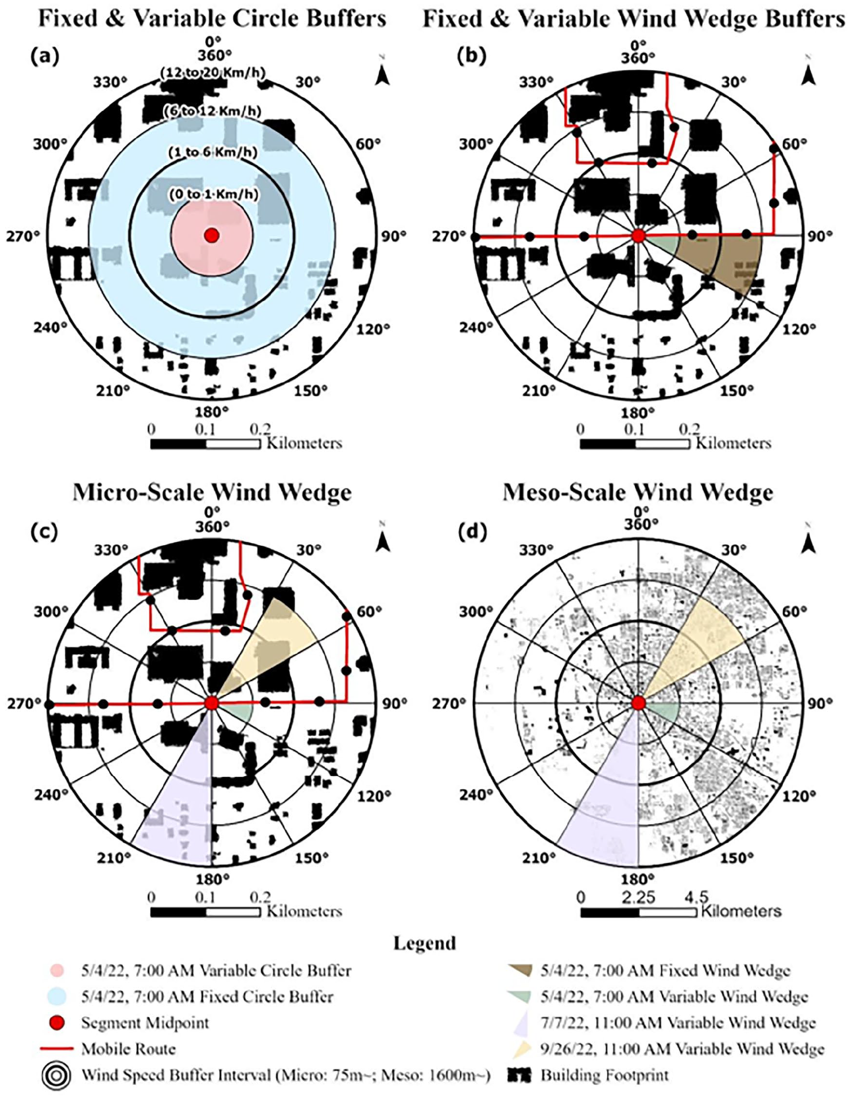
Graphic illustration of eight different buffer methods. (a) presents the fixed and variable circle buffers and (b) shows the fixed and variable wind wedge buffers. Each of the four methods in (a) and (b) will be calculated at (c) micro-scale and (d) meso-scale.

Furthermore, we defined two distinct spatial scales to quantify the landscape-air pollution relationship at the micro and meso scales. The micro scale is characterized by local distance intervals ranging from 75 m to 450 m, while the macro scale is defined by regional distance intervals ranging from 1,600 m to 9,600 m, both in accordance with wind speed changes (Figure 3). Buffer interval ranges were constructed based on similar buffers in the literature (Table S1; Gilliland et al., 2018; Gulliver et al., 2016; Hart et al., 2020; Hu et al., 2021; Tang et al., 2013).

We established wind speed-based radii and a respective buffer direction, corresponding with hourly wind-related changes. For determining the wind wedge, we first discretized the 360° wind field into a set of 12 30° wind wedges. The direction of the wedge depends on the wind direction, and the radius of the wedge relies on the wind speed. To determine the radius, we first categorized wind speeds (measured in km/h) into six levels according to the Beaufort Wind force scale (Hausman, 1978): 0–1 km/h, 1–6 km/h, 6–12 km/h, 12–20 km/h, 20–29 km/h, and 29–39 km/h. Buffer radii varied based on the scale of interest. For the micro scale, the buffer radii were calculated by multiplying the wind force scale by a factor of 75 m, resulting in radii ranges from 75 m to 450 m. For the meso scale, the factor increased to 1600 m, resulting in radii ranges from 1600 m to 9600 m. In cases where wind data was unavailable for a specific sample route segment, we used a circle buffer with a fixed radius of 25 meters. For each segment, we used the midpoint as either the centroid of circle buffer, or the vertex of the wedge for generating the different buffers. All steps were conducted using the QGIS 3.26 Wedge Buffer tool. The average and standard deviation of vegetation and building heights, as well as the summation of vegetation and building footprints, were calculated within the buffers using the zonal statistics tool in Esri’s ArcGIS Pro 3.4.

Explanatory model development

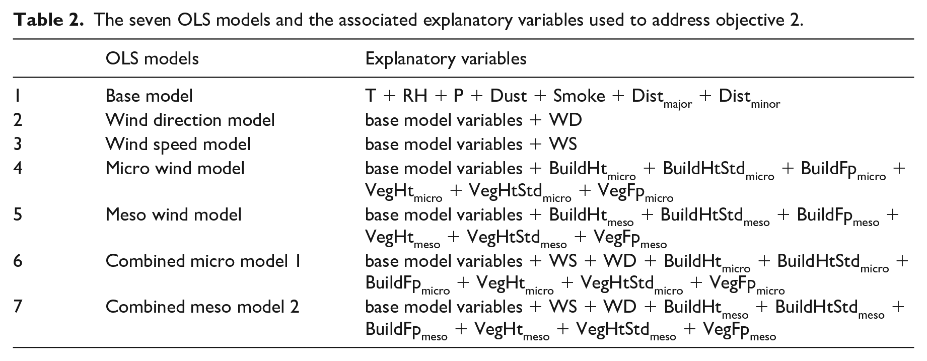
We used a set of ordinary least squares regression (OLS) models to assess the effectiveness of different buffer types in capturing the variation in PM_2.5 (Table 2). Utilizing the set of predictor variables, 19 models were developed and evaluated using coefficient of determination (R²), adjusted R² (for measuring the variation for a multiple regress model), Root Mean Squared Error (RMSE), Akaike information criterion (AIC), and Bayesian information criterion (BIC). The first model, referred to the “base model”, comprises seven explanatory variables that we set as base variables, separately temperature, relative humidity, sea-level pressure, distance to major roads, distance to minor roads, presence of smoke or dust, and the season (hereafter referred to as the “base variables”). Additional models were created that supplanted base variables with 1) wind speed variables, 2) wind direction variables, 3) micro-scale built environment, 4) meso-scale built environment, and models that combined wind-related variables with either micro- or meso-scale variables (5 & 6). It is worth noting that the last four models were fitted with built environment variables calculated using four different buffers, resulting in a total of 16 models.

Table 2.

The seven OLS models and the associated explanatory variables used to address objective 2.

	OLS models	Explanatory variables
1	Base model	T + RH + P + Dust + Smoke + Dist_major + Dist_minor
2	Wind direction model	base model variables + WD
3	Wind speed model	base model variables + WS
4	Micro wind model	base model variables + BuildHt_micro + BuildHtStd_micro + BuildFp_micro + VegHt_micro + VegHtStd_micro + VegFp_micro
5	Meso wind model	base model variables + BuildHt_meso + BuildHtStd_meso + BuildFp_meso + VegHt_meso + VegHtStd_meso + VegFp_meso
6	Combined micro model 1	base model variables + WS + WD + BuildHt_micro + BuildHtStd_micro + BuildFp_micro + VegHt_micro + VegHtStd_micro + VegFp_micro
7	Combined meso model 2	base model variables + WS + WD + BuildHt_meso + BuildHtStd_meso + BuildFp_meso + VegHt_meso + VegHtStd_meso + VegFp_meso

Because the light-scattering devices are sensitive to the ambient environment, especially humidity (Liang 2021; Liang and Daniels 2022), data collected under humidity conditions greater than 80% were removed. Similarly, to reduce outlier influence from street hotspots, the top 20% of PM_2.5 concentrations were removed, reducing the total sample size from 6,399 to 4,427. Afterward, normalization and standardization were applied to all explanatory and response variables. Normalization was performed by subtracting the minimum values of all variables from each element of the variables to set the minimum value of each variable to zero, leveling variables to a similar scale while reducing the influence of extreme values. Standardization subtracts the mean and divides by the standard deviation of each variable, resulting in z-scores for each variable, enabling comparison of relative magnitudes for different variables in our analysis. Each seasonal dataset had a sample size of 2,160 unique segments, and the overall dataset had a combined sample size of 6,480.

Model selection and development

Previous studies have explored panel data analysis model for mobile monitoring dataset with longitudinal and time-series dimensions. However, after a series of tests, we found that Ordinary Least Squares (OLS) regression was more suitable than both fixed and random effects model. While OLS is commonly used to assess the relationship between variables, this study aimed to generate OLS variations by substituting potential predictors and observed the changes in $R^{2}$ values to determine the effectiveness of different buffer techniques in capturing the spatial-temporal PM_2.5 variation. By comparing the $R^{2}$ of the other models with the base model (Table 2), we can evaluate the impact of the added variables in other models.

Results and discussion

Spatial-temporal variation of PM_2.5

In general, our multi-seasonal mobile monitoring data indicated a declining PM_2.5 trend throughout the day, with peak concentrations observed at 7 AM, reaching the lowest levels at 3 PM across all three seasons, and slight increases at 7 PM (Figure 4). This contrasts previous understanding of diurnal behaviors in the study area that suggested a gradual increase in PM_2.5 throughout the day (Hart et al., 2020). The elevated 7 AM concentration in Spring and Fall corresponds to morning rush hour on Interstate-35 (Transportation Planning & Programming Division, & Texas Department of Transportation, 2016), and 11 AM had higher levels in Spring than Summer, potentially due to increased student traffic during school sessions. At 3 PM, concentrations were consistently low across all seasons, likely attributed to the low traffic volume at that time. Overall, the diurnal variation on the university campus closely followed traffic patterns, assuming no other major emission sources were present.

Figure 4.

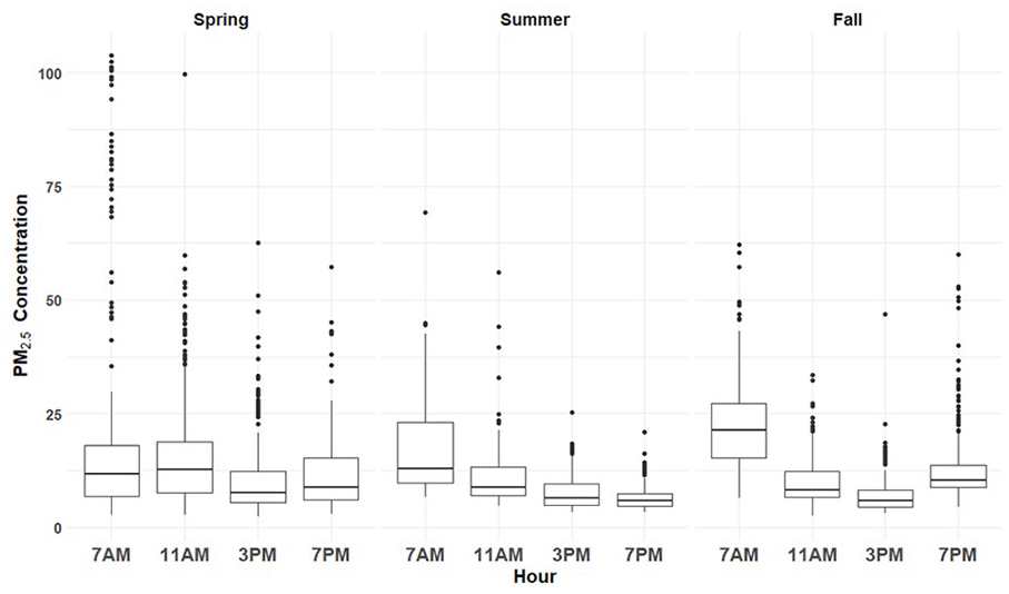
Box plot illustrating PM_2.5 concentration (μg/m³) variations at each data collection hour throughout three seasons.

The spatial pattern of street-level PM_2.5 suggests the possibility of microenvironment hotspots, primarily influenced by construction sites and dining halls (Figure 5). This observation is in accordance with previous studies (Harr et al., 2022; Hwang and Lee, 2018). During Spring and Summer, elevated concentrations were observed at a southwestern construction site, while a new hotspot emerged in the Fall at the northern route section. Cooking activities elevate PM_2.5 concentrations throughout all seasons, with smoke events recorded east of the campus union building in the Spring and in the central portion during Summer and Fall. Additionally, other factors, like grass mowing and idling stops near traffic lights, influence air quality on the campus. These hotspots, being a natural component of urban street environments and critically influential in human exposure, are frequently overlooked by fixed monitoring stations, underscoring the distinctive advantage of mobile air quality monitoring.

Figure 5.

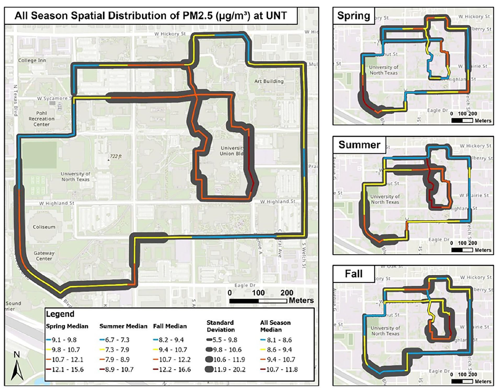
Median and standard deviation of PM_2.5 concentrations (μg/m³) along the sampling route. Colors indicate variable medians and the grey buffers indicate standard deviation range.

Effect of wind buffer choice on PM_2.5 model performance

The four buffer methods demonstrated minimal discrepancies in influencing model performance, with variations in R² estimates amounting to 1% or less in predictive differences (Table 3). This observation also remained true for adjusted R² (Table S3). The base model explained 46.0% of the variation in Spring, and the inclusion of the micro-scale variable wind wedge only led to a marginal increase to 46.6%. The variable circle buffer showed the most improvement but contributed to only an additional 1.2% to explain the model variation in the Fall. Additionally, AIC and BIC values exhibited negligible differences across all buffer methods (Table S3). With minimal variance among the wind buffer methods, only the variable wind wedge buffer calculated built environment variables were used in Objective 2.

Table 3.

Comparison of predictability potential of different wind-based buffers.

Wind buffer	R²				RMSE
Wind buffer	Spring	Summer	Fall	Overall	Spring	Summer	Fall	Overall
Variable wind wedge (Micro)	0.466	0.375	0.389	0.298	0.731	0.790	0.782	0.838
Variable circle (Micro)	0.462	0.38	0.389	0.299	0.733	0.787	0.782	0.837
Fixed wind wedge (Micro)	0.464	0.381	0.389	0.301	0.732	0.787	0.781	0.836
Fixed circle (Micro)	0.463	0.379	0.389	0.299	0.732	0.788	0.781	0.838
Variable wind wedge (Meso)	0.464	0.372	0.389	0.298	0.732	0.792	0.782	0.838
Variable circle (Meso)	0.464	0.38	0.401	0.298	0.732	0.788	0.774	0.838
Fixed wind wedge (Meso)	0.464	0.373	0.389	0.298	0.732	0.791	0.781	0.838
Fixed circle (Meso)	0.461	0.376	0.391	0.297	0.734	0.790	0.780	0.838

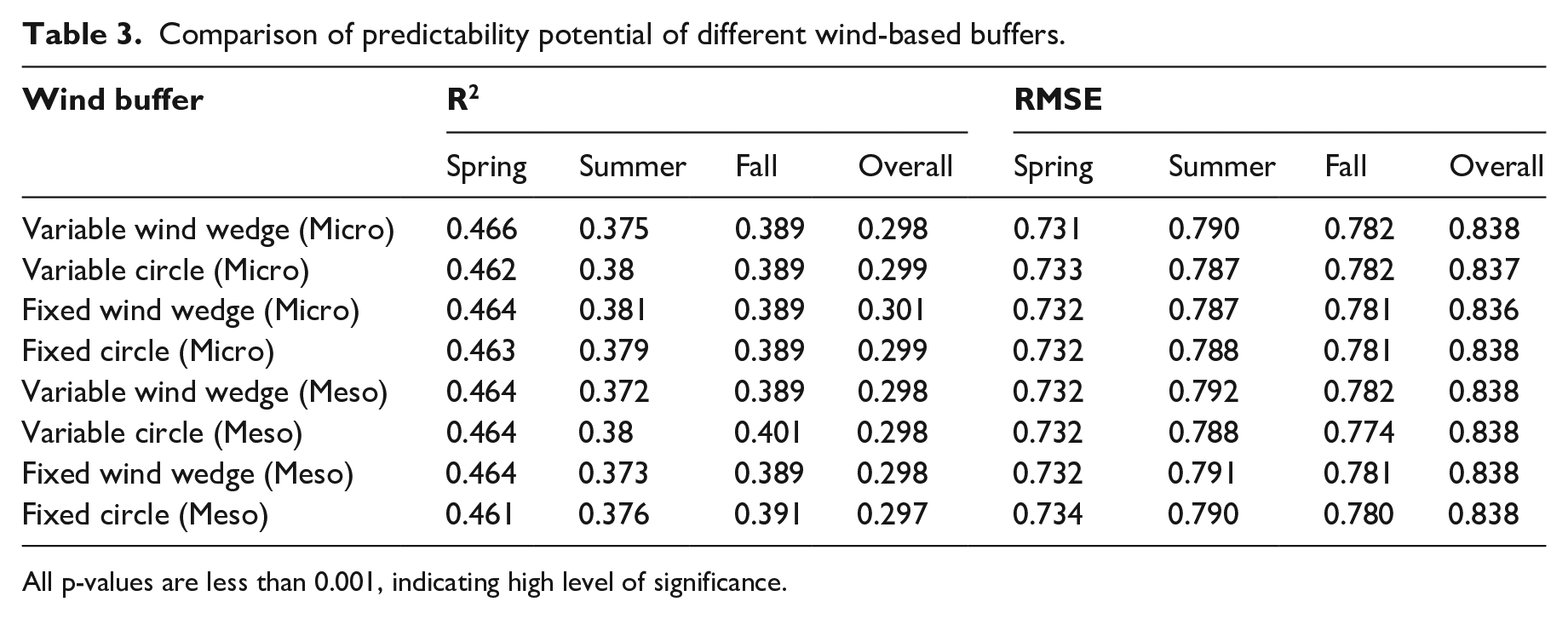
All p-values are less than 0.001, indicating high level of significance.

Effect of built environment on PM_2.5 variation

Although some previous studies have proposed that wind patterns and spatial form may influence PM_2.5 differently depending on scale (Kim et al., 2015; Naughton et al., 2018), we found no significant differences in the influence of built environment between micro- and meso-scale. The inclusion of micro-scale built environment variables only marginally improved the base model’s predictive capacity by 0.06% in Spring, 0.05% in Summer, 0.02% in Fall, and 0.02% in the Overall dataset (Figure 6). In addition, the micro-scale buffer model only slightly outperformed the meso-scale by 0.02% and 0.03% in Spring and Summer, respectively, and had no effect in the Fall and Overall datasets. Unlike densely packed cities with tall buildings like Hong Kong or New York City, Denton primarily consists of a suburban residential landscape with low- to middle-rise buildings. Consequently, changes in building height are less dramatic, and the street canyon effect is less evident. Moreover, unlike urban areas with distinct topography, such as the Beijing Tianjin-Hebei region (Wen et al., 2022), Denton’s relatively flat topography may facilitate the easy movement of particulates (Chen et al., 2020). Overall, these findings suggest that built environment plays a less substantial role in influencing PM_2.5 levels in Denton, compared to other factors such as local emission hotspots or wind-driven dynamics.

Figure 6.

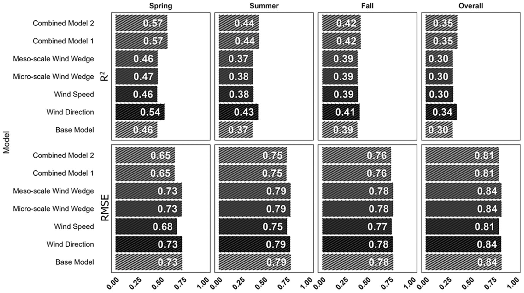
Comparison of R² values from the seven ordinary least squares regression models.

Given the significance of wind direction in shaping PM_2.5 concentrations and the limited impact of local built environment, our findings indicate that regional wind dynamics play a considerably larger role in determining PM_2.5 levels in Denton compared to the 3D structure of the local area. Regional dynamics have been documented in previous studies (Huang et al., 2017; Xu et al., 2020), and the transport of particulates from upwind to downwind regions has been observed in scenarios such as wildfires (Aguilera et al., 2020) and intercity pollution (Gilliland et al., 2018; Kim et al., 2015). Our findings emphasize that urban planning should involve collaboration with neighboring urban complexes to tackle air pollution on a regional scale. Such collaborative efforts have shown to yield positive effects on downwind concentrations, as evidenced by previous studies (Aguilera et al., 2020; Kim et al., 2015).

Effect of wind speed and direction on PM_2.5 variation

Upon comparing the various OLS models, the highest R² values were consistently observed in the Spring dataset (0.46–0.574), followed by Fall (0.387–0.423) and Summer (0.37–0.443), with the Overall dataset showing the lowest values (0.296–0.348) (Figure 6). Notably, despite the Spring dataset having the highest R² estimates, it showcased substantial variation among different models, underscoring the significant impact of variable selection. Subsequent sections will explore the discrepancies in R² estimates across the models. In addition, the lowest AIC and BIC values are consistently found in the Spring dataset across different models. This might suggest that in the context of this study, the Spring conditions (such as weather patterns, human activities, or other environmental factors) might be better captured by the models, or that the data quality is higher in this season for some reason. Of all the models, AIC and BIC values for the combined models and “base + wind direction” are lower than all other model choices, implying that the complexity added by combining models is justified by a corresponding increase in the goodness of fit. This is especially the case given the limited change observed in adjusted R² values.

In this case study, wind speed exhibits a restricted impact on PM_2.5 variation, with no alteration to R² values in Spring, a marginal increase of 0.09% in Summer, a 0.06% rise in Fall, and a 0.07% increase in the Overall dataset. While some studies underscored the importance of wind speed (Requia et al., 2019), we found the pronounced influence of prevailing wind direction on predicting PM_2.5 variation, which aligns with some earlier research findings (Gilliland et al., 2018; Miao et al., 2020). Wind direction enhanced the model predictability by 8% in Spring, 6.4% in Summer, 2.5% in Fall, and 4.6% in the overall dataset. Moreover, the wind direction-derived model displayed little to no difference in corresponding adjusted R² coefficients. This indicates that the inclusion of wind direction as a predictor significantly improved model explanatory power without overfitting. Furthermore, of the 13 total models, the base model supplanted with wind direction consistently showed one of the lowest AIC and BIC values of all 13 models (Figure S4, S5), surpassed only by the combined models, which incorporated the wind direction variable themselves. This underscores wind direction’s importance in predictive accuracy. In turn, we observed the tendency of PM_2.5 concentrations to elevate in the south-southeasterly direction of the prevailing wind (Figure 7). This pattern is particularly pronounced in Spring, with median concentrations of 9.9 µg/m³ in the southeast and 11.8 µg/m³ in the south (Figure 8). Although the Spring southwestern median is notably high (17.4 µg/m³), its sample size was limited and thus removed from the models in the analysis. The dominant impact of wind direction might be attributed to regional-level wind dynamics in the absence of pronounced urban morphology effects. When wind originates from more industrialized urban centers, the downwind areas often experience elevated air pollution (Gilliland et al., 2018; Guerra et al., 2006), thereby escalating the risk of cross-regional air pollution (Xu et al., 2020). The growth and traffic activities in the urban cores of Dallas and Fort Worth likely significantly impact concentration fluctuations in Denton. Moreover, prevailing wind patterns transport PM_2.5 from these areas to Denton, a process exacerbated by this area’s low elevation, which facilitates the particle movement.

Figure 7.

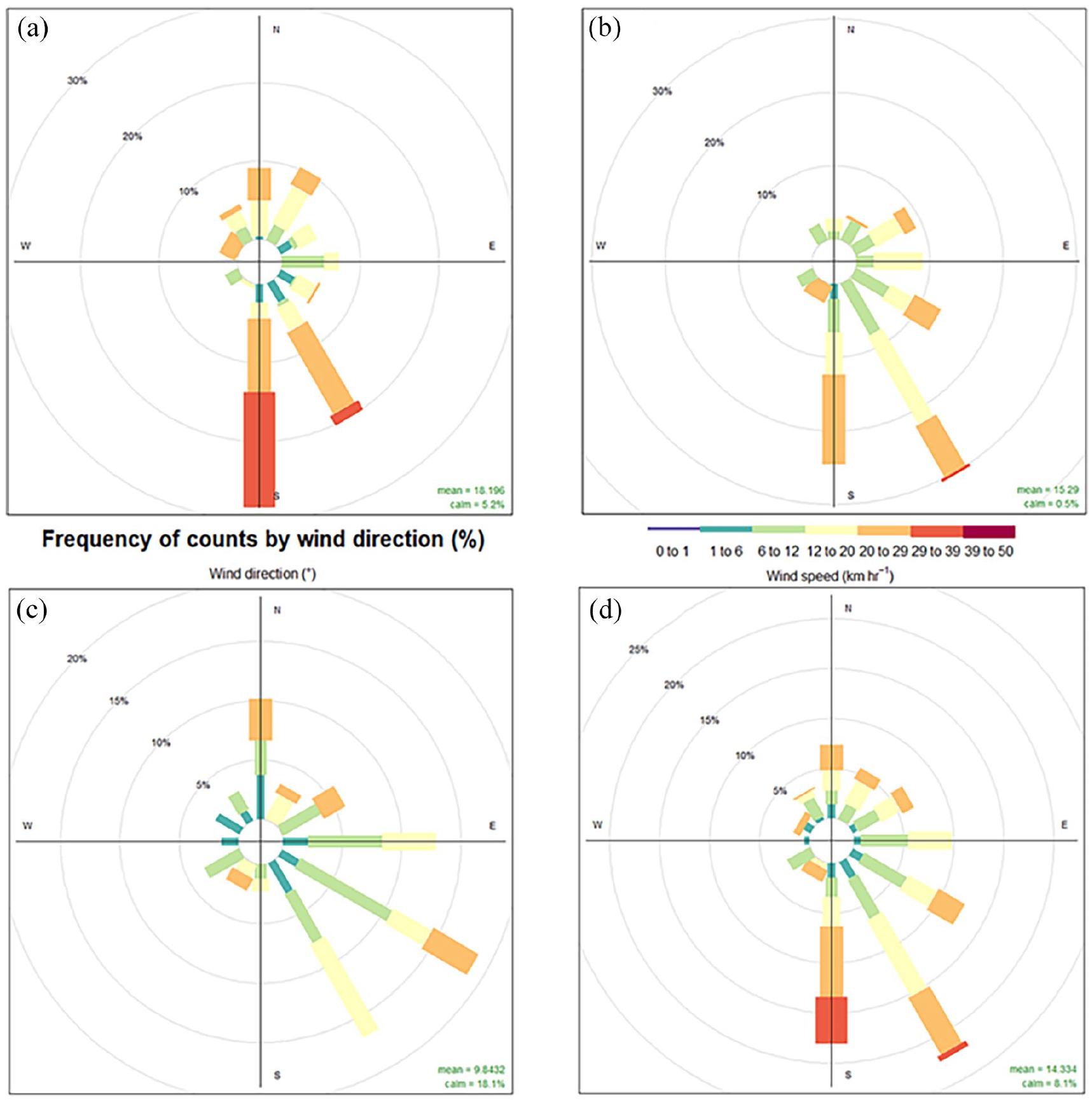
Seasonal wind rose plots: (a) Spring, (b) Summer, (c) Fall, and (d) Overall model. Wind rose is colored based on the Beaufort wind force scale.

Figure 8.

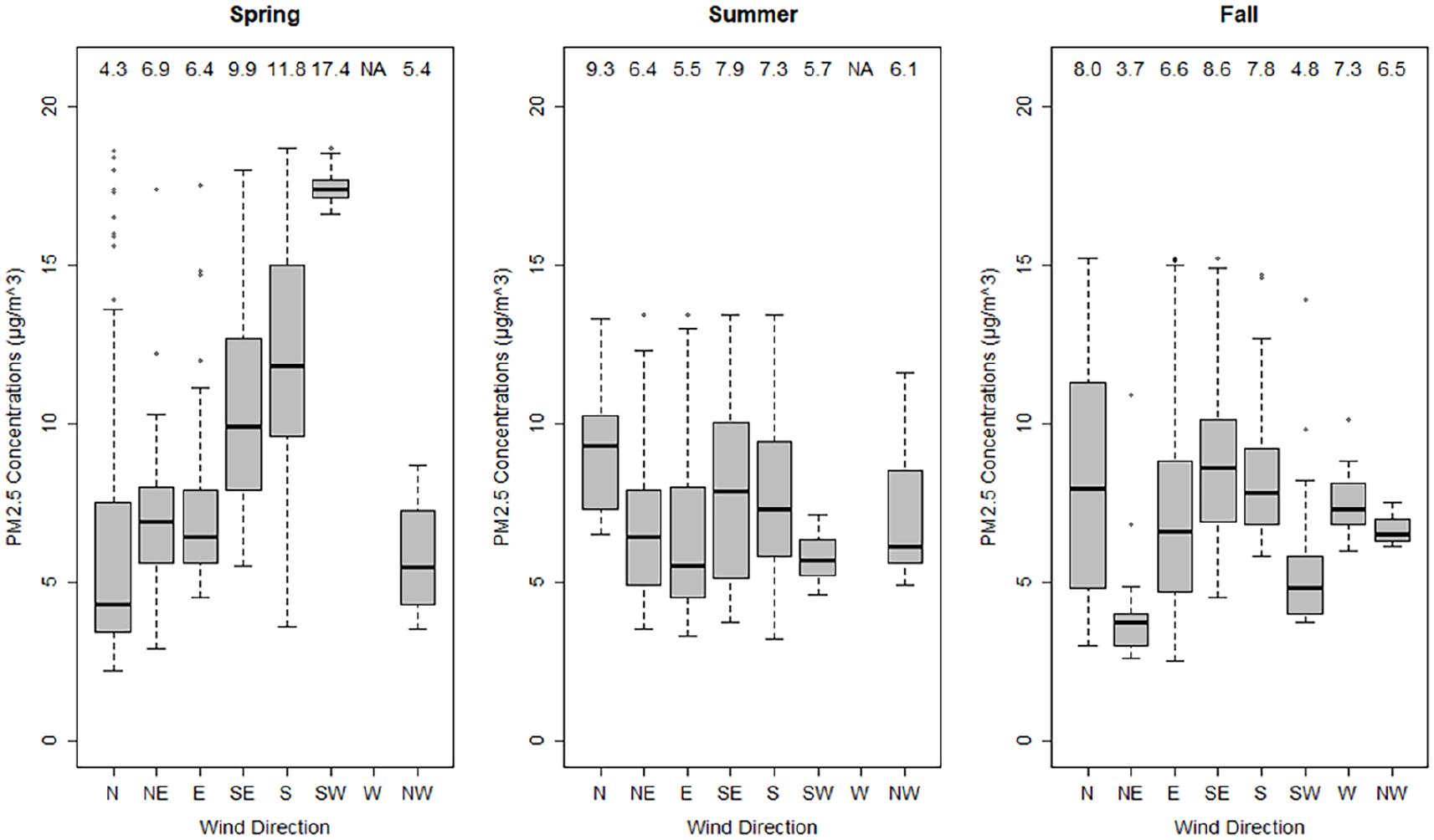
Seasonal median PM_2.5 concentrations in each wind direction. Median concentration values are listed on the top portion of each seasonal plot.

Limitations

This study exhibits several weaknesses. Firstly, with our study area being confined to a university campus, while holding significant public health implications, its spatial scope may not be able to fully capture the effects of built environment, given that other studies analyze urban form over several cities and investigate much more unique forms of urban structures (Li and Zhou, 2019). Moreover, Denton’s landscape, featuring relatively low building canopy, further indicates that the impact of built environment within such a confined study area might be limited. Accuracy of meteorological variables was another concern in this study. Rising temperature was responsible for significantly reducing PM_2.5 in the Fall, but the opposite was the case for the Spring and Summer. This dynamic was complicated by relative humidity significantly increasing the PM_2.5 concentrations in the Spring and Summer, but not in the Fall. Simple regression analysis of the source station revealed that temperature changes significantly altered PM_2.5 concentrations during the study period, but the same was not true for relative humidity. At the same time, low-cost sensors are highly affected by local and street level temperature and humidity changes, which were not accounted for by our sampling procedure. Such dynamics should be clarified using robust meteorological data inputs (Miao et al., 2020). Another potential oversight in this study is that the dominance of a particular wind direction on the variation of PM_2.5 levels may be the product of confounding variables not accounted for in this study. Notably, unmeasured factors in this study, such as traffic volume, may have demonstrated a significant effect on PM_2.5 concentrations, correlating with observed variations. Additionally, the tendency for PM_2.5 concentrations to decline over longer distances may contradict the long-range transport hypothesis in certain conditions. Yet, the statistical performance of wind direction across all seasons suggests some level of statistical relationship, specifically in study contexts similar to ours, with similar topographies and urban layouts. Finally, when accounting for wind speed effects, we made the simplifying assumption that particle transport follows a linear distance pattern, while overlooking the potential influence of dilution and dry or wet deposition, which could alter this relationship (Lee et al., 2019; Oke et al., 2017). Future studies should adopt a more sophisticated approach to model these dynamics for a more realistic and accurate representation.

Conclusion

This research offers a unique insight into PM_2.5 variation at a very high spatial-temporal resolutions on a university campus through multi-seasonal mobile monitoring, which is still relatively rare in current studies (Liu et al., 2020; Song et al., 2022; Tiwari and Aljoufie, 2021). We examined the impacts of wind-dynamics at both the micro scale and the meso scale, and evaluated the statistical efficacy of 3D built environment variables obtained through four novel wind-based buffer methods in the OLS models. Although the four methods did not reveal significant differences and the effect of built environment remained limited, this could possibly be attributed to Denton’s flat terrain and relatively low city skylines. Further studies should explore the applicability of these methods within more heterogeneous urban areas.

Moreover, because the inclusion of wind variables into OLS models may result in varied model performance from season to season, a method to calibrate season-specific wind frequency into wind-based buffer models is encouraged (Naughton et al., 2018). One noteworthy discovery from our study was the dominant influence of wind direction on changes in PM_2.5 concentrations. This influence outweighed the importance of wind speed as a driving factor and may have interacted with the orientation of the pollutant source. As incorporating wind direction into models can be complex, our approach of utilizing the eight cardinal directions may also offer a computationally efficient technique to account for wind direction’s role in emission dispersion.

Supplemental Material

sj-docx-1-tus-10.1177_27541231241248858 – Supplemental material for Wind-urban structure interplay in PM2.5 variation: Insights from multi-seasonal mobile air quality campaign

Supplemental material, sj-docx-1-tus-10.1177_27541231241248858 for Wind-urban structure interplay in PM2.5 variation: Insights from multi-seasonal mobile air quality campaign by Noah Ray, Pinliang Dong, John South and Lu Liang in Transactions in Urban Data, Science, and Technology

Footnotes

Acknowledgements

The authors would like to thank many student volunteers at the University of North Texas for the mobile air quality sampling. Special thanks to Ronan Hart at Utah State University for providing pilot study data, as well as to Dr. Wei Kang for her valuable comments and insightful suggestions throughout the course of this project.

Declaration of conflicting interests

The author(s) declared no potential conflicts of interest with respect to the research, authorship, and/or publication of this article.

Funding

The author(s) disclosed receipt of the following financial support for the research, authorship, and/or publication of this article: This project is supported by the National Science Foundation (BCS-2117505).

Supplemental material

Supplemental material for this article is available online.

Author biographies

Noah Ray received his MS degree in Geography from the University of North Texas in 2023. He is currently a GIS Specialist/Developer for the Texas Natural Diversity Database at Texas Parks and Wildlife. His primary research interests encompass environmental and spatial modeling, urban pollution-transport dynamics, and species distribution modeling.

Pinliang Dong received his PhD degree in Geology from the University of New Brunswick in 2003. He is currently a Professor at the Department of Geography and the Environment, University of North Texas, USA. His research interests include geographic information systems and LiDAR applications in Earth science and urban environments.

John South is a geospatial information scientist whose research is focused on the use of unmanned aerial vehicles in combination with LiDAR and satellite imagery to observe the structural and compositional impacts of human interaction with the environment. He is also researching the application of deep learning models to spatial analysis. He is a Part 107 certified professional UAV pilot. He is currently a PhD student and full-time lecturer at the University of North Texas.

Lu Liang received her PhD degree from the Department of Environmental Science, Policy, and Management at the University of California, Berkeley. She is currently an associate professor in the Department of Landscape Architecture and Environmental Planning at the University of California, Berkeley. Her research focuses on geospatial and environmental science.

References

Abhijith

Kumar

Gallagher

, et al. (2017) Air pollution abatement performances of green infrastructure in open road and built-up street canyon environments: A review. Atmospheric Environment 162: 71–86.

Aguilera

Gershunov

Ilango

, et al. (2020) Santa Ana winds of Southern California impact PM_2.5 with and without smoke from wildfires. GeoHealth 4(1): e2019GH000225.

Alzuhairi

Aldhaheri

Sun

, et al. (2016) Vehicular emissions and concentrations in school zones: A case Study. Journal of Central South University 23(7): 1778–1785.

Apte

Messier

Gani

, et al. (2017) High-resolution air pollution mapping with Google street view cars: Exploiting big data. Environmental Science & Technology 51(12): 6999–7008.

Ariunsaikhan

Chonokhuu

Matsumi

(2020) Mobile measurement of PM_2.5 based on an individual in Ulaanbaatar city. International Journal of Environmental Research and Public Health 17(8): 2701.

Stowell

Seto

, et al. (2020) Contribution of low-cost sensor measurements to the prediction of PM2. 5 levels: A case study in Imperial County, California, USA. Environmental Research 180: 108810.

Bryant

(2021) How bad is the air in Denton? Enough to turn off some businesses. Available at: dentonrc.com. Available at: https://dentonrc.com/news/environmental_issues/how-bad-is-the-air-in-denton-enough-to-turn-off-some-businesses/article_e450aa7f-25de-5c11-aab1-28486d27ae35.html (accessed 24 April 2024).

Cao

Rui

Liang

(2018) Study on PM_2.5 pollution and the mortality due to lung cancer in China based on geographic weighted regression model. BMC Public Health 18(1): 1–10.

Charron

Harrison

(2005) Fine (PM2. 5) and coarse (PM2. 5-10) particulate matter on a heavily trafficked London highway: Sources and processes. Environmental Science & Technology 39(20): 7768–7776.

10.

Chatzidimitriou

Yannas

(2017) Street canyon design and improvement potential for urban open spaces; the influence of canyon aspect ratio and orientation on microclimate and outdoor comfort. Sustainable Cities and Society 33: 85–101.

11.

Chen

Zhao

, et al. (2020) Influence of meteorological conditions on PM_2.5 concentrations across China: A review of methodology and mechanism. Environment International 139: 105558.

12.

Chowdhury

Dey

(2016) Cause-specific premature death from ambient PM2. 5 exposure in India: Estimate adjusted for baseline mortality. Environment International 91: 283–290.

13.

City of Denton (2022) Statistical trends and news of Denton. Available at: www.cityofdenton.com/DocumentCenter/View/8592/Qtr-4-FY-22-23-STaND (accessed 24 April 2024).

14.

Cohen

Brauer

Burnett

, et al. (2017) Estimates and 25-year trends of the global burden of disease attributable to ambient air pollution: An analysis of data from the Global Burden of Diseases Study 2015. The Lancet 389(10082): 1907–1918.

15.

Dadvand

Rivas

Basagaña

, et al. (2015) The association between greenness and traffic-related air pollution at schools. Science of the Total Environment 523: 59–63.

16.

Denton County

(2022) Roads. Available at: https://data-dentoncounty.hub.arcgis.com/datasets/DentonCounty::roads-1/explore?location=33.205802%2C-97.150188%2C15.51 (accessed 24 April 2024).

17.

Erlandson

Magzamen

Carter

, et al. (2019) Characterization of indoor air quality on a college campus: a pilot study. International Journal of Environmental Research and Public Health 16(15): 2721.

18.

Fruin

Westerdahl

Sax

, et al. (2008) Measurements and predictors of on-road ultrafine particle concentrations and associated pollutants in Los Angeles. Atmospheric Environment 42(2): 207–219.

19.

Gilliland

Maltby

, et al. (2018) Influence of the natural and built environment on personal exposure to fine particulate matter (PM2. 5) in cyclists using city designated bicycle routes. Urban Science 2(4): 120.

20.

Gulliver

de Hoogh

Hoek

, et al. (2016) Back-extrapolated and year-specific NO₂ land use regression models for Great Britain-Do they yield different exposure assessment? Environment International 92: 202–209.

21.

Harr

Sinsel

Simon

, et al. (2022) Seasonal changes in urban PM2. 5 hotspots and sources from low-cost sensors. Atmosphere 13(5): 694.

22.

Hart

Liang

Dong

(2020) Monitoring, mapping, and modeling spatial–temporal patterns of PM_2.5 for improved understanding of air pollution dynamics using portable sensing technologies. International Journal of Environmental Research and Public Health 17(14): 4914.

23.

Hausman

(1978) Specification tests in econometrics. Econometrica: Journal of the Econometric Society 46(6): 1251–1271.

24.

Huang

Zhang

(2017) Development of land use regression models for PM_2.5, SO₂, NO₂ and O₃ in Nanjing, China. Environmental Research 158: 542–552.

25.

Huang

Hou

Liu

, et al. (2019) Effects of wind direction on the airflow and pollutant dispersion inside a long street canyon. Aerosol and Air Quality Research 19(5): 1152–1171.

26.

Chen

Qian

, et al. (2021). Impacts of traffic and street characteristics on the exposure of cycling commuters to PM_2.5 and PM₁₀ in urban street environments. Building and Environment 188: 107476.

27.

Belle

Meng

, et al. (2017) Estimating PM2.5 concentrations in the conterminous United States using the random forest approach. Environmental Science & Technology 51(12): 6936–6944.

28.

Hwang

Lee

(2018) Contribution of microenvironments to personal exposures to PM₁₀ and PM_2.5 in summer and winter. Atmospheric Environment 175: 192–198.

29.

Karra

Malki-Epshtein

Neophytou

(2017) Air flow and pollution in a real, heterogeneous urban street canyon: A field and laboratory study. Atmospheric Environment 165: 370–384.

30.

Huang

, et al. (2022) Three-dimensional building morphology impacts on PM_2.5 distribution in urban landscape settings in Zhejiang, China. Science of the Total Environment 826: 154094.

31.

Kerckhoffs

Hoek

Messier

, et al. (2016) Comparison of ultrafine particle and black carbon concentration predictions from a mobile and short-term stationary land-use regression model. Environmental Science & Technology 50(23): 12894–12902.

32.

Kim

Lee

Woo

, et al. (2015) Influence of wind direction and speed on the transport of particle-bound PAHs in a roadway environment. Atmospheric Pollution Research 6(6): 1024–1034.

33.

Lee

Hong

Lee

, et al. (2019) Ceilometer monitoring of boundary-layer height and its application in evaluating the dilution effect on air pollution. Boundary-layer Meteorology 172: 435–455.

34.

Dallmann

, et al. (2016) Application of mobile sampling to investigate spatial variation in fine particle composition. Atmospheric Environment 142: 71–82.

35.

Liu

Chen

, et al. (2015) The application of semicircular-buffer-based land use regression models incorporating wind direction in predicting quarterly NO₂ and PM₁₀ concentrations. Atmospheric Environment 103: 18–24.

36.

Fung

Lau

(2018) High spatiotemporal characterization of on-road PM_2.5 concentrations in high-density urban areas using mobile monitoring. Building and Environment 143: 196–205.

37.

Liang

(2021) Calibrating low-cost sensors for ambient air monitoring: Techniques, trends, and challenges. Environmental Research 197: 111163.

38.

Liang

Daniels

(2022) What influences low-cost sensor data calibration? A systematic assessment of algorithms, duration, and predictor selection. Aerosol and Air Quality Research 22(9): 220076.

39.

Liang

Daniels

Bailey

, et al. (2023) Integrating low-cost sensor monitoring, satellite mapping, and geospatial artificial intelligence for intra-urban air pollution predictions. Environmental Pollution 331: 121832.

40.

Zhou

(2019) Effects of urban form on air quality in China: An analysis based on the spatial autoregressive model. Cities 89: 130–140.

41.

Liu

Cai

Zhu

, et al. (2020) Impacts of vehicle emission from a major road on spatiotemporal variations of neighborhood particulate pollution—a case study in a university campus. Sustainable Cities and Society 53: 101917.

42.

Meng

Chen

Cai

, et al. (2015) A land use regression model for estimating the NO₂ concentration in shanghai, China. Environmental Research 137: 308–315. DOI: 10.1016/j.envres.2015.01.003.

43.

Messier

Chambliss

Gani

, et al. (2018) Mapping air pollution with Google Street View cars: Efficient approaches with mobile monitoring and land use regression. Environmental Science & Technology 52(21): 12563–12572. DOI: 10.1021/acs.est.8b03395.

44.

Zhuang

Zhang

, et al. (2019) Spatiotemporal characteristics of PM_2.5 and its associated gas pollutants, a case in China. Sustainable Cities and Society 45: 287–295.

45.

Miao

, et al. (2020) How the morphology of urban street canyons affects suspended particulate matter concentration at the pedestrian level: An in-situ investigation. Sustainable Cities and Society 55: 102042.

46.

Miskell

Salmond

Longley

, et al. (2015) A novel approach in quantifying the effect of urban design features on local-scale air pollution in central urban areas. Environmental Science & Technology 49(15): 9004–9011.

47.

Naughton

Donnelly

Nolan

, et al. (2018) A land use regression model for explaining spatial variation in air pollution levels using a wind sector based approach. Science of the Total Environment 630:1324–1334.

48.

NOAA National Centers for Environmental Information (2022) Climate Data Online Search. Available at: https://www.ncdc.noaa.gov/cdo-web/search (accessed 24 April 2024).

49.

Oke

Mills

Christen

, et al. (2017) Urban Climates. Cambridge: Cambridge University Press.

50.

Park

Han

, et al. (2021) Intra–community scale variability of air quality in the center of a megacity in South Korea: A high-density cost-effective sensor network. Applied Sciences 11(19): 9105.

51.

Qiu

Zhang

, et al. (2019) Pedestrian exposure to PM_2.5, BC and UFP of adults and teens: A case study in Xi’an, China. Sustainable Cities and Society 51: 101774.

52.

Requia

Jhun

Coull

, et al. (2019) Climate impact on ambient PM_2.5 elemental concentration in the United States: A trend analysis over the last 30 years. Environment International 131: 104888.

53.

She

Peng

, et al. (2017) Air quality and its response to satellite-derived urban form in the Yangtze River Delta, China. Ecological Indicators 75: 297–306.

54.

Shi

Ren

Lau

, et al. (2019) Investigating the influence of urban land use and landscape pattern on PM_2.5 spatial variation using mobile monitoring and WUDAPT. Landscape and Urban Planning 189: 15–26.

55.

Snyder

Watkins

Solomon

, et al. (2013) The changing paradigm of air pollution monitoring. Environmental Science & Technology 47(20): 11369–11377.

56.

Song

Zhou

Peng

, et al. (2022) Relationship between neighborhood land use structure and the spatiotemporal pattern of PM_2.5 at the microscale: Evidence from the central area of Guangzhou, China. Environment and Planning B: Urban Analytics and City Science 49(2): 485–500.

57.

Tang

Blangiardo

Gulliver

(2013) Using building heights and street configuration to enhance intraurban PM₁₀, NO_X, and NO2 land use regression models. Environmental Science & Technology 47(20): 11643–11650.

58.

Tsiaperas

(2022) Dallas-Fort Worth leads the nation in population growth. Available at: www.axios.com/local/dallas/2022/03/31/dallas-fort-worth-2021-population-growth (accessed 24 April 2024).

59.

Tian

Yao

Chen

(2019) Analysis of spatial and seasonal distributions of air pollutants by incorporating urban morphological characteristics. Computers, Environment and Urban Systems 75: 35–48.

60.

Tiwari

Aljoufie

(2021) Modeling spatial distribution and determinant of PM_2.5 at micro-level using geographically weighted regression (GWR) to inform sustainable mobility policies in campus based on evidence from King Abdulaziz University, Jeddah, Saudi Arabia. Sustainability 13(21): 12043.

61.

Tong

Shi

, et al. (2021) Mapping microscale PM_2.5 distribution on walkable roads in a high-density city. IEEE Journal of Selected Topics in Applied Earth Observations and Remote Sensing 14: 6855–6870.

62.

Transportation Planning & Programming Division, & Texas Department of Transportation (2016) I-35 Statewide Corridor Plan: A Path to 2040. Available at: https://ftp.txdot.gov/pub/txdot/my35/planning/corridor-plan.pdf (accessed 24 April 2024).

63.

UNT News Service (2022) UNT spring enrollment climbs 6% to over 40k for first time as Tier One Research University status is reaffirmed. Available at: https://news.unt.edu/news-releases/unt-spring-enrollment-climbs-6-over-40k-first-time-tier-one-research-university-status (accessed 24 April 2024).

64.

U.S. Census Bureau (2022) QuickFacts Denton city, Texas.. Available at: www.census.gov/quickfacts/fact/table/dentoncitytexas/LND110210 (accessed 2023).

65.

Van Poppel

Peters

Bleux

(2013) Methodology for setup and data processing of mobile air quality measurements to assess the spatial variability of concentrations in urban environments. Environmental Pollution 183: 224–233. DOI: 10.1016/j.envpol.2013.02.020

66.

Vodonos

Awad

Schwartz

(2018) The concentration-response between long-term PM_2.5 exposure and mortality; A meta-regression approach. Environmental Research 166: 677–689.

67.

Wang

Cheng

Dai

(2022) Strategies for sustainable urban development and morphological optimization of street canyons: Measurement and simulation of PM_2.5 at different points and heights. Sustainable Cities and Society 87: 104191.

68.

Weissert

Alberti

Miskell

, et al. (2019) Low-cost sensors and microscale land use regression: Data fusion to resolve air quality variations with high spatial and temporal resolution. Atmospheric Environment 213: 285–295.

69.

Wen

Xiao

Yang

, et al. (2022) Quantitatively disentangling the geographical impacts of topography on PM_2.5 pollution in China. Remote Sensing 14(24): 6309.

70.

World Health Organization (WHO) (2018) Air quality, energy and health. www.who.int/teams/environment-climate-change-and-health/air-quality-energy-and-health/sectoral-interventions/ambient-air-pollution/health-risks (accessed 24 April 2024).

71.

Chen

(2021). Impact of urban morphology on the spatial and temporal distribution of PM_2.5 concentration: A numerical simulation with WRF/CMAQ model in Wuhan, China. Journal of Environmental Management 290: 112427.

72.

Ren

Xiong

, et al. (2020) Analysis of the driving factors of PM_2.5 concentration in the air: A case study of the Yangtze River Delta, China. Ecological Indicators 110: 105889.

73.

Yuan

Song

Huang

, et al. (2019) Exploring the association between the built environment and remotely sensed PM_2.5 concentrations in urban areas. Journal of Cleaner Production 220: 1014–1023.

74.

Zhang

Xia

(2022) Exploring the effects of 3D urban form on urban air quality: Evidence from fifteen megacities in China. Sustainable Cities and Society 78: 103649. DOI: 10.1016/j.scs.2021.103649.

75.

Zhang

Jiao

, et al. (2018) Influences of wind and precipitation on different-sized particulate matter concentrations (PM_2.5, PM₁₀, PM_2.5–10). Meteorology and Atmospheric Physics 130(3): 383–392.

76.

Zhou

Lin

(2019) Spatial-temporal heterogeneity of air pollution: The relationship between built environment and on-road PM_2.5 at micro scale. Transportation Research Part D: Transport and Environment 76: 305–322.

Supplementary Material

Please find the following supplemental material available below.

For Open Access articles published under a Creative Commons License, all supplemental material carries the same license as the article it is associated with.

For non-Open Access articles published, all supplemental material carries a non-exclusive license, and permission requests for re-use of supplemental material or any part of supplemental material shall be sent directly to the copyright owner as specified in the copyright notice associated with the article.

0.00 MB

0.94 MB

Wind-urban structure interplay in PM 2.5 variation: Insights from multi-seasonal mobile air quality campaign

Abstract

Keywords

Introduction

Study area

Methods

Mobile monitoring campaign

Field sampling and data collection

Data preprocessing

Explanatory variables

Meteorological variables

Proximity to traffic

Local pollution sources

LiDAR data for analyzing 3D built environment

Developing wind wedge-based buffers at micro- and meso- scale for urban built environment

Explanatory model development

Model selection and development

Results and discussion

Spatial-temporal variation of PM2.5

Effect of wind buffer choice on PM2.5 model performance

Effect of built environment on PM2.5 variation

Effect of wind speed and direction on PM2.5 variation

Limitations

Conclusion

Supplemental Material

sj-docx-1-tus-10.1177_27541231241248858 – Supplemental material for Wind-urban structure interplay in PM2.5 variation: Insights from multi-seasonal mobile air quality campaign

Footnotes

Acknowledgements

Declaration of conflicting interests

Funding

Supplemental material

Author biographies

References

Supplementary Material

Spatial-temporal variation of PM_2.5

Effect of wind buffer choice on PM_2.5 model performance

Effect of built environment on PM_2.5 variation

Effect of wind speed and direction on PM_2.5 variation