Sage Journals: Discover world-class research

Abstract

Understanding population dynamics at fine spatiotemporal granularities are valuable to human-centered studies. With the increasing availability of high-frequency human digital footprint data, the past decades have witnessed numerous efforts in mapping populations at fine spatiotemporal scales. However, such research still lacks a unified standard in modeling strategy and auxiliary data selection, especially a systematic comparison between newly developed machine learning techniques and traditional spatial statistical methods under different covariates provisions. Here, we compared two spatial statistical models, the Bayesian space-time model and geographically and temporally weighted regression, with two machine learning techniques, random forest and eXtreme gradient boosting, in a case study of hourly population mapping at 100 m resolution in Beijing. We evaluated the model performance with varied covariates combinations and found that the Bayesian space-time model achieved the best in conjunction with urban function data. Leveraging the optimal model constructed, we mapped dynamic population distribution and concluded human activity patterns on diverse city amenities. This paper emphasizes the importance of spatiotemporal dependency information in fine temporal scale population mapping and the urban function covariates in urban population mapping.

Keywords

Human dynamic population mapping machine learning spatial statistics Beijing

Introduction

Today, more than half of the world’s population—4.2 billion inhabitants—live in urban areas (World Bank, 2020). Rapid urbanization brings great economic, cultural, and societal benefits but also challenges to city and community sustainable development (Klopp and Petretta, 2017). Understanding population dynamics, therefore, plays a crucial role in human-centered urban studies, typically for disaster management (Smith et al., 2019), infectious diseases prevention (Tatem et al., 2012), and urban planning (Song et al., 2021). However, the main source for the demographic data from the national census and housing survey is hard to meet policymakers’ and researchers’ requirements due to infrequent updates and coarse spatial granularities, thereby encouraging studies of modeling population dynamics at fine spatiotemporal scales (Stevens et al., 2015; Leyk et al., 2019). More recently, the human digital footprint data, such as mobile phone positioning records and geotagged social media posts, provides unprecedented opportunities to achieve this point (Chen et al., 2018; Deville et al., 2014; Zhao et al., 2021), leading to population mapping products with temporal resolution spans from decadal (Gaughan et al., 2016; Wang et al., 2018), annual (WorldPop, Landscan), monthly (Cheng et al., 2022), to daily (Tu et al., 2022), which enables a better understanding of the population dynamics (Panczak et al., 2020).

Disproportionally reallocating census data to fine-scale grid squares (known as “top-down” downscaling) via the association between population count and auxiliary variables is the mainstream methodological framework in population mapping research (Wardrop et al., 2018; Leasure et al., 2020). With the increasing popularity of machine learning techniques applied in spatial predictive modeling (Hengl et al., 2017, 2018; Bi et al., 2019), a growing number of studies adopted and assumed that fitting nonlinear relationships using these models could improve prediction accuracy than traditional statistical methods, leading to their explosive and even excessive use in population mapping research (Stevens et al., 2015; Patel et al., 2017; Yao et al., 2017; Ye et al., 2019; Zhao et al., 2021). However, despite some neural network-based models having accommodated the geographical space, widely adopted tree-based machine learning approaches, such as random forest, mostly ignore the spatial structure of the population distribution. They commonly lack sufficient consideration on neither spatial autocorrelation that geostatistics focuses on (Cheng et al., 2022) nor varied spatial relations emphasized by spatial local modeling, such as geographically weighted regression (Bagan and Yamagata, 2015; Chen et al., 2019; Liu et al., 2021; Wang et al., 2018). Little evidence supports that the nonlinear relationship always overweighs the importance of spatial characteristics of population distribution in the model.

More recently, there has been an increasing interest in understanding how the characteristics of covariates impact the dynamic population mapping—this study contributes to this effect (Lloyd et al., 2017, 2019). It is commonly accepted that the models could approach the real population distribution more accurately with the increasing of covariates related to human activity, particularly for the data-driven machine learning methods. However, some studies have reminded us that we should be cautious about applying excessive covariates in spatial modeling. For exampling, Samuel-Rosa et al. (2015) showed that more covariates have no necessary association with higher accuracy in soil mapping, but instead increase the burden of data preparation. However, in the field of population modeling, it is still an open question as to which dimension of covariates counts more in improving the mapping accuracy. In other words, distinct influences of covariates on dynamic population mapping still lack real-world comparison, leaving their pros and cons across methods unclear.

Here, we evaluated the performance of spatial statistical and machine learning models with different combinations of covariates in urban dynamic population mapping. We took Beijing as a testing site to model the hourly population distribution at a spatial resolution of 100 m. Taking the linear regression model (LM) as the benchmark, we compared four widely used methods: two machine learning approaches, random forest and eXtreme Gradient Boosting (XGBoost), and two spatial statistical models, Bayesian space-time model and geographically and temporally weighted regression (GTWR). The machine learning approaches excel in capturing the nonlinear relationship between population distribution and covariates, while the spatial statistical models could take the spatiotemporal autocorrelation and varied spatial relationship into the models. To examine whether more covariates deliver more accurate population mapping, we introduced 18 auxiliary variables in five categories—human digital footprint, terrain, land use, urban morphology, and urban function to the five models and evaluated the model performance when those covariates were progressively added. Besides the human digital footprint data essential for dynamic population mapping, we found urban function data remarkably reduced population estimates bias. With the help of these covariates, the Bayesian space-time model achieved the best performance. However, methods of machine learning techniques in our case are more stable, with no prominent estimation error, in the absence of urban function data. Lastly, we reconstructed the hourly population dynamics for one week and highlighted distinct visitation laws across different amenities in the city. Overall, this paper provides empirical evidence for urban dynamic population mapping model designs, helping better understand the urban problems and facilitating sustainable development.

Data

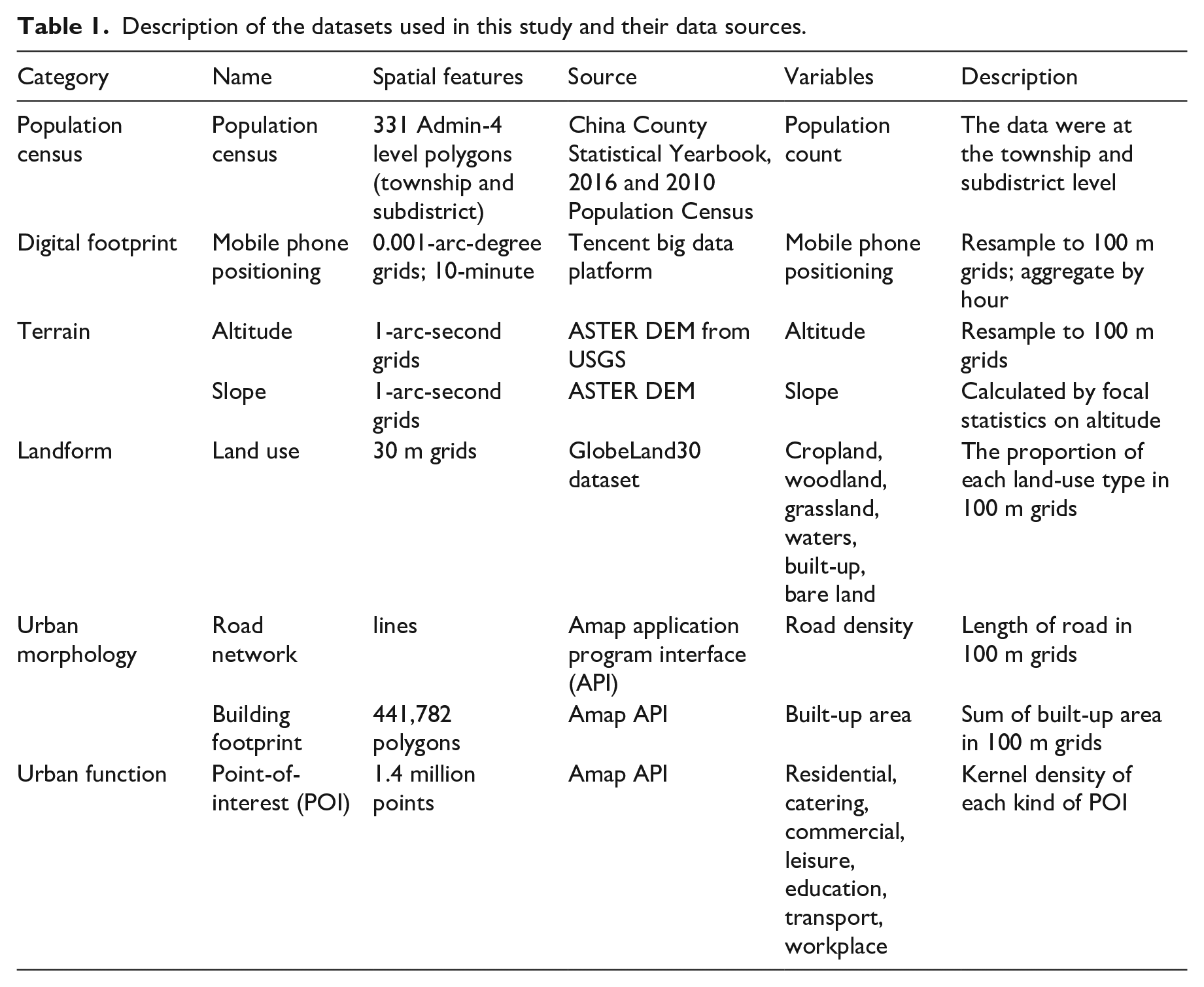
We collected data closest to 2015 to realize dynamic population mapping. The residential population of administrative units was collected from official statistics, serving as a baseline for population downscaling. The covariates were derived from the following six datasets: mobile phone positioning, terrain, land use, road network, building footprint, and point-of-interest (POI), as summarized in Table 1.

Table 1.

Description of the datasets used in this study and their data sources.

Category	Name	Spatial features	Source	Variables	Description
Population census	Population census	331 Admin-4 level polygons (township and subdistrict)	China County Statistical Yearbook, 2016 and 2010 Population Census	Population count	The data were at the township and subdistrict level
Digital footprint	Mobile phone positioning	0.001-arc-degree grids; 10-minute	Tencent big data platform	Mobile phone positioning	Resample to 100 m grids; aggregate by hour
Terrain	Altitude	1-arc-second grids	ASTER DEM from USGS	Altitude	Resample to 100 m grids
Terrain	Slope	1-arc-second grids	ASTER DEM	Slope	Calculated by focal statistics on altitude
Landform	Land use	30 m grids	GlobeLand30 dataset	Cropland,woodland,grassland,waters,built-up,bare land	The proportion of each land-use type in 100 m grids
Urban morphology	Road network	lines	Amap application program interface (API)	Road density	Length of road in 100 m grids
Urban morphology	Building footprint	441,782 polygons	Amap API	Built-up area	Sum of built-up area in 100 m grids
Urban function	Point-of-interest (POI)	1.4 million points	Amap API	Residential,catering,commercial,leisure,education,transport,workplace	Kernel density of each kind of POI

Census

Census data commonly serves as a reliable data source of population statistics. Here we collected the residential population in 2015 at the admin-4 level (a township in rural and a subdistrict in urban zoning) in Beijing. Data for 142 townships were collected from ‘China County Statistical Yearbook, 2016’, and that for 189 subdistricts were derived by intuitively multiplying the census in 2010 by the annual population growth rate of the corresponding upper-level admin-3 unit. We subsequently joined our census data with administrative boundaries through unique identifiers.

Mobile phone positioning data

The Tencent big data center provides mobile phone location datasets depicting footprints of online activities. As one of the largest internet companies in China, it periodically records people’s locations when using location-based services (such as check-in, online ride-hailing, and nearby searching) on social media Apps, including Wechat and QQ. Their extremely high popularity in China, with more than 700 million users in 2015, ensures a low sample bias across ages, income, and education levels. In this study, we obtained mobile location data from Tencent’s big data platform “Easygo”, which reports anonymous and aggregated mobile phone positioning data with a spatial resolution of 0.001° on a 10-minute basis. The data covered one week period (from July 12 to July 18, 2015) in Beijing. We then aggregated them to one-hour temporal resolution and resampled them to a spatial resolution of 100 m by the nearest neighbor method.

Terrain

We collected ASTER DEM from the United States Geological Survey (USGS, https://earthexplorer.usgs.gov/) to describe basic regional topography. Taking tiles of original data with a spatial resolution of 1″ (approximately 28m at Beijing), we mosaiced, reprojected, and resampled them to produce an average altitude on regular grids of 100 m resolution. We later calculated the average surface slope for each grid based on their adjacent eight neighbors by adopting a 3×3 focal moving window.

Land use

We collected land-use data with a spatial resolution of 30 m from the GlobeLand30 ( http://www.globallandcover.com/). We identified eight land-use categories within Beijing: cropland, woodland, grassland, shrubland, wetland, waters, built-up area, and bare land. To eliminate categories with limited area, we first merged shrubland with woodland and merged wetland with waters. Then we resampled the resultant six categories into a spatial resolution of 100 m and generated the area proportion of each land-use type in 100 m grids. The resampling process simultaneously converted the original categorical data into continuous data, which benefits the following analysis.

Road network

Convenient transportation is significant to daily commuting and public services accessibility, thus usually attracting population gathering. This study obtained city road network data comprising three levels: state road, arterial road, and urban street, from the Amap API (https://ditu.amap.com/). Taking the DEM data as a template, we calculated road length within each 100 m grid cell and named the resultant raster layer as road density. We discarded highways in our analysis due to their weak relevance to people’s daily lives.

Building footprints

We obtained building footprint data for 441,782 buildings in Beijing from the Amap. The original data records the building shapes and the number of floors. We extracted the footprint area of each building and calculated the built-up area by multiplying the respective number of floors. Similar to the road network, we subsequently calculated the gross built-up area in each 100 m grid to represent build density in a certain region.

Point-of-interest

Laws of population dynamics across different venues might vary by their functions, function density, and spatial gathering, which opts to play a crucial role in inner-city, high-frequency population mapping. However, land-use data seldom reveal those details. In this study, we collected more than 1.4 million POIs from the Amap to depict urban functional zones. According to the Amap POIs lookup table, we selected 700 thousand POIs that fall into seven categories: residential, catering, commercial, leisure, education, transport, and workplace. Then, we calculated the kernel density of each category by adopting a Gaussian kernel model with a bandwidth of 150 m, which covers the 3×3 neighborhood of each grid. The resultant layers represent the spatial clustering of different venues.

Methods

The general framework of dynamic population mapping

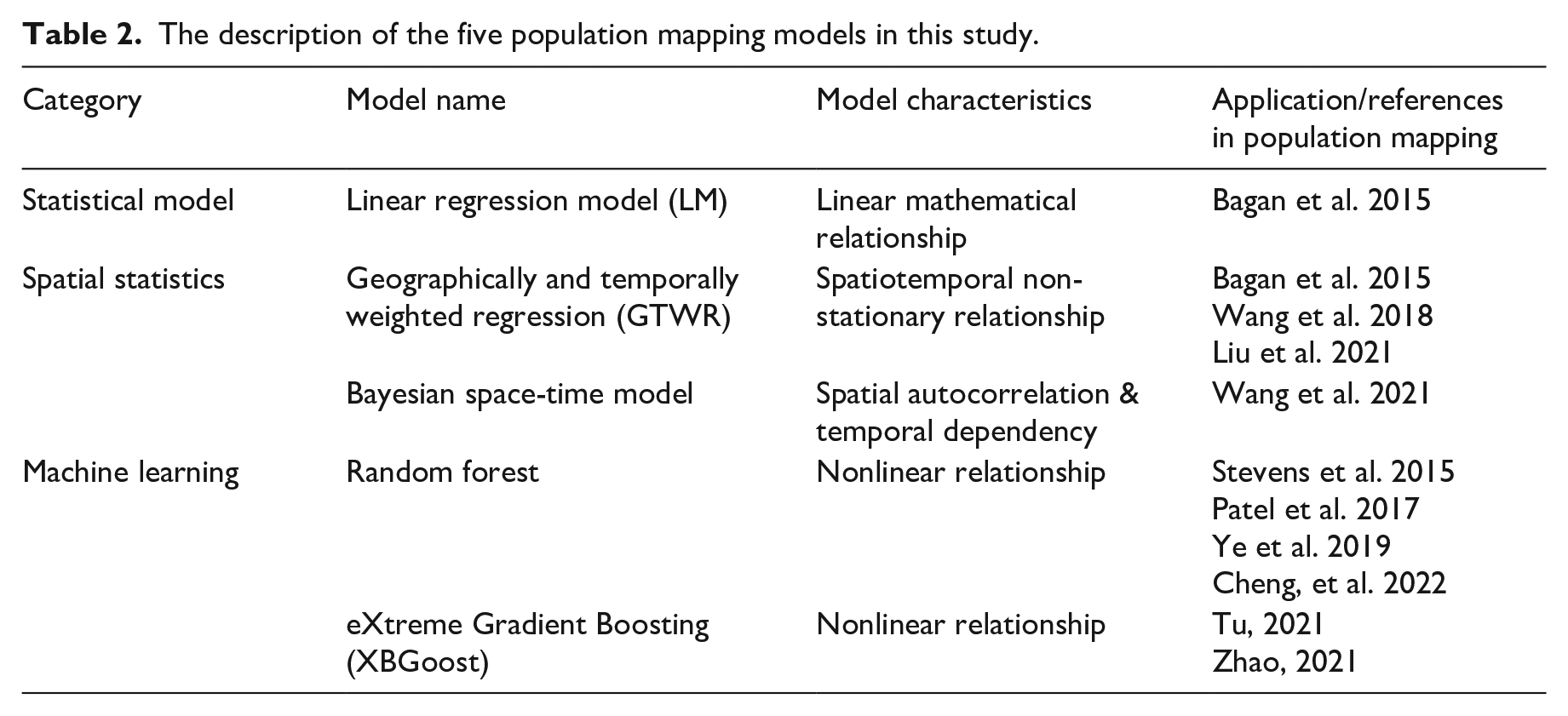
We aim to evaluate five models’ performance with different covariates for hourly population mapping. See Table 2 for the description of the five models. Due to inactive mobile phone activity and stable population distribution at midnight, we restricted our modeling to 6 am to 11 pm each day. To cope with the absence of the true population count at the targeted fine scale, we constructed our models at the admin-4 level unit and then applied them to estimate the population on each grid. However, the static residential population from census data is hard to satisfy the dynamic population demand. We, therefore, took the mobile phone positioning data to adjust the real-time population count for each administrative unit in each hour in the first place (see section “Adjust census data”). We deemed this data directly derived from human activity to be a reliable source reflecting population movement.

Table 2.

The description of the five population mapping models in this study.

Category	Model name	Model characteristics	Application/references in population mapping
Statistical model	Linear regression model (LM)	Linear mathematical relationship	Bagan et al. 2015
Spatial statistics	Geographically and temporally weighted regression (GTWR)	Spatiotemporal non-stationary relationship	Bagan et al. 2015 Wang et al. 2018 Liu et al. 2021
Spatial statistics	Bayesian space-time model	Spatial autocorrelation & temporal dependency	Wang et al. 2021
Machine learning	Random forest	Nonlinear relationship	Stevens et al. 2015 Patel et al. 2017 Ye et al. 2019 Cheng, et al. 2022
	eXtreme Gradient Boosting (XBGoost)	Nonlinear relationship	Tu, 2021Zhao, 2021

We took the average population density for each administrative unit as the response variable and the corresponding mean value of covariates as explanatory variables during the modeling construction procedure. We tried different covariates combinations to clarify the effects of various covariates on population estimation. For each covariates combination, we established five models: LM, GTWR, Bayesian space-time model, random forest, and XGBoost. Amongst these, we estimated the population for each hour separately when using LM, random forest, and XGBoost, but fed a day’s worth of data together as input when using the Bayesian space-time model and GTWR. Finally, we integrated models and covariates to estimate the population on each 100 m grid for each hour and then evaluated the consistency of our results with population statistics.

Adjust census data

We determined the population for each administrative unit at a certain hour by adjusting census data with mobile phone positioning data. The population change ratio is defined as the shift in the share of mobile phone positioning. The formula is specified as

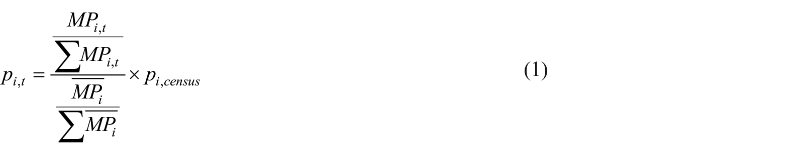
p_{i, t} = \frac{\frac{M P_{i, t}}{\sum M P_{i, t}}}{\frac{\bar{M P_{i}}}{\sum \bar{M P_{i}}}} \times p_{i, c e n s u s}

(1)

where i ranges from 1,2, to 331 (number of census tracts, see Table. 1), $p_{i, t}$ is the population count of administrative unit i at time t, $p_{i, c e n s u s}$ is its resident population count obtained from census data, $M P_{i, t}$ is the number of mobile phone positioning in unit i at time t, and $\bar{M P_{i}}$ is the average number of mobile phone positioning in unit i in one day.

When executing census adjustment, we assumed that the mobile phone activity for each specific town are comparable over time. However, population flow between administrative units and the resulting fluctuation in the relationship between mobile phone active users and the real population was ignored.

Evaluate the contribution of covariates

We divided the covariates into five categories in the dynamic population mapping (see Table 1): topography (altitude and slope), land use (proportion of six land-use types at 100 m resolution), urban morphology (road density and built-up area distribution), urban function (kernel density of seven types of POIs), and human digital footprint (number of mobile phone positioning). We set the model with only mobile phone positioning data as the baseline or benchmark and then progressively added the other four categories of covariates into the model. We evaluated the model performance with the mapping accuracy to determine each variable’s contribution. To eliminate the potential multicollinearity, we assessed Pearson correlations between covariates and discarded existing covariates with collinearity when adding a new type of covariates. For instance, we removed the proportion of built-up land-use types when urban morphology data was added due to the strong correlation. Similarly, the built-up area distribution in urban morphology was also discarded when incorporating urban function data.

Population mapping models

Linear regression model

The linear regression (LM) model is a simple method in regression analysis. It assumes invariant and additive relationships between the response and explanatory variables and generates estimated coefficients with the smallest residuals by ordinary least-squares fitting. The formula could be written as

Y = β_{0} + β X + ε

(2)

where $Y$ represents a vector of average population densities for administrative units in this study, $X$ is a matrix of corresponding mean values of covariates, $β_{0}$ is the regression intercept, $β$ is a vector of regression coefficients for each covariate, and $ε$ is a random error term.

Geographically and temporally weighted regression

The geographically and temporally weighted regression (GTWR) is an approach to detecting non-stationary spatiotemporal relationships (Fotheringham et al., 2015). As an extension of the linear regression model, it uses a kernel to move within the study area and execute local regression, allowing relationships between the response and explanatory variables to vary rather than be consistent in space and time. Its general format can be represented as

Y_{i t} = β_{0, i t} + β_{i t} X_{i t} + ε_{i t}

(3)

where $Y_{i t}$ is the population density of unit i at time t, $X_{i t}$ is a vector of mean values of covariates in unit i at time t, $β_{0, i t}$ is the regional regression intercept, and $β_{i t}$ is a vector of regression coefficients for covariates at i^th location at time t.

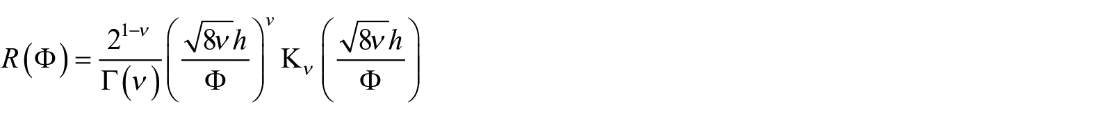
Bayesian space-time model

The separatable space-time model under the Bayesian framework has a hierarchical structure of three levels (Blangiardo et al., 2013; Bakka et al., 2018). In the first level, we assumed the population density to follow a log-normal prior distribution

p_{i t} ~ L o g N o r m a l (μ_{i t}, σ_{i t})

(4)

where ~ represents the prior distribution obeyed, $p_{i t}$ represents the population density of unit i at time t, $μ_{i}$ represents the expected population based on covariates at location i at time t, and $σ_{i}$ is the random variation that could not be explained by covariates.

Next, we defined the expected population as a linear combination of an invariant intercept $β_{0, i t}$ , a set of fixed covariate effects $β_{i t} X_{i t},$ a spatially correlated innovation $S_{i t}$ , a first-order autoregressive dynamics $ω_{i t}$ , and an independent nugget effect $ε_{i t}$ in the second-level process model

μ_{i t} = β_{0, i t} + β_{i t} X_{i t} + S_{i t} + ω_{i t} + ε_{i t}

(5)

where $β_{0, i t}$ is the regression intercept and $β_{i t}$ is the posterior coefficient of covariates. Finally, we specified the prior distribution assumptions for each component in the third-level parameter model

S_{i t} ~ G P (0, Σ_{s p a c e})

Σ_{s p a c e} = τ^{- 1} R (Φ)

R (Φ) = \frac{2^{1 - ν}}{Γ (ν)} {(\frac{\sqrt{8 ν} h}{Φ})}^{v} Κ_{ν} (\frac{\sqrt{8 ν} h}{Φ})

ω_{i t} = ρ ω_{i (t - 1)}

P (ρ > 0) = 0.9

ε_{i} ~ N o r m a l (0, σ_{n u g g e t}^{2})

where $S_{i t}$ represents the spatial random effect, which is specified as an isotropic Gaussian process with mean 0 and a Matérn covariance matrix. $τ^{- 1}$ is the marginal covariance, $R (Φ)$ is the Matérn correlation function, $h$ is the relative distance between any pair of locations, $Φ$ indicates the maximum range where autocorrelation approaches zero, $Γ$ is the gamma function, and $Κ_{ν}$ is the modified Bessel function of the second kind with order $ν > 0$ . Next, we defined the temporal autoregressive component to have first-order autocorrelation with prior probability $ρ$ larger than 90%. Finally, the residual estimation error follows a Gaussian distribution with a mean of 0.

Random forest

Random forest is a data-driven method that has been widely adopted in the predictive modeling of spatial variables (Breiman, 2001). Instead of falling into explicit, complex mathematical formulations, it takes bagged decision trees as the basic classifiers, samples variables independently to train each tree, and generates final decisions through majority voting or averaging results. This solving strategy favors nonlinear relationship detection and avoidance of overfitting.

We established random forest models using data for each hour as input. Each time when trying a new covariates combination, we fine-tuned the number of trees in the forest and the number of covariates selected by each node of each tree. The fine-tuning procedure minimizes the out-of-bag (OOB) error and guarantees the minimal estimation error.

eXtreme Gradient Boosting (XGBoost)

XGBoost ensembles decision tree and gradient boosting (Chen and Guestrin, 2016). Instead of training a set of trees independently and adopting an additive function to obtain final predictions, like the random forest model, it greedily takes the best results of the previous tree and fits a new tree on its residuals.

L^{(t)} = \sum_{i = 1}^{N} l (y_{i} {\hat{y_{i}}}^{(t - 1)} + f_{t} (x_{i})) + Ω (f_{t})

(6)

where l is the loss function that measures the difference between prediction and the reality, $y_{i}$ is the observation and ${\hat{y_{i}}}^{(t - 1)}$ is the prediction at (t-1)^th iteration. $f_{t} (x_{i})$ represents the new decision tree trained at t^th time. $Ω (f_{t})$ is a cost function that penalizes the complexity of the model, thereby avoiding overfitting. Particularly, XGBoost takes second-order approximation through Taylor expansion to absorb more previous information instead of merely first-order. Therefore, the above formula can be written as

L^{(t)} ≅ \sum_{i = 1}^{N} [l (y_{i} {\hat{y_{i}}}^{(t - 1)}) + g_{i} f_{t} (x_{i}) + \frac{1}{2} h_{i} f_{t}^{2} (x_{i})] + Ω (f_{t})

(7)

where $g_{i}$ and $h_{i}$ is the first- and second-order gradient statistics on the loss function, respectively. More information is provided by Chen and Guestrin (2016).

Like the random forest, we trained XBGoost models in this paper by using data for each hour as input separately. We randomly leave 10% of our sample to calculate the loss function. Each time when trying a new covariates combination, we determined a new threshold of iteration to avoid overfitting.

Model performance assessment

We assessed the model performance from two aspects. First, we compared our estimation with statistical data. Owing to the absence of real population count at a certain hour on either a specific grid or a spatial extent finer than modeling, we summarized our estimated population to the admin-4 level unit (the same as model construction) and compared them with the adjusted hourly statistical population count. We then used 10-fold cross-validation to avoid duplicated use of training data and test the extrapolating ability of models. Two commonly used indicators, coefficient of determination (R²) and root-mean-squared-error (RMSE), were adopted as quality measurements.

R M S E = \sqrt{\frac{1}{n} \sum_{i = 1}^{n} (\hat{y_{i}} - Y_{i})}

(8)

R^{2} = \frac{\sum_{i} {(\hat{y_{i}} - \bar{y})}^{2}}{\sum_{i} {(y_{i} - \bar{y})}^{2}}

(9)

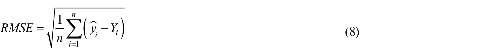
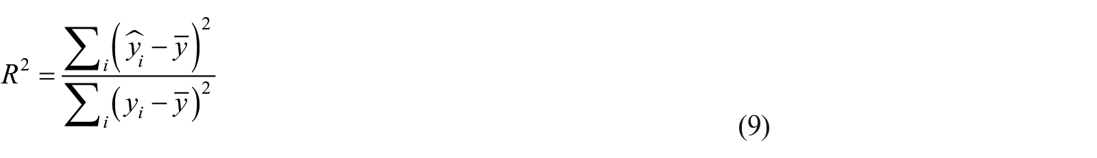
where R² approaches 1 represents a higher consistency, and lower RMSE represents less estimation bias.

We then presented the changes in population distribution patterns with the progressive addition of different covariates. This pair-comparison could help clarify the effect of covariates from the mechanism. We can see how different covariates make population estimates to be spatially clustered, sparsely distributed, or empty in a certain place. Figure 3 shows more details of this.

Results

Evaluate the model performance

We evaluated the performance of five population dynamic mapping models by adding covariates gradually. The model performance was evaluated by two statistical indicators: the coefficient of determination (R²) and the root-mean-squared-error (RMSE). We set the LM model containing only mobile phone positioning data as the baseline model. Then, we compared R² and RMSE with the baseline by progressively adding auxiliary variables, including terrain, land use, urban morphology, and urban functions (see Table 1). The R² index was compared with its absolute values, while RMSE was compared with its relative changes.

Figure 1a shows the results of models’ performance with different covariates. The R² of the five models varies in a similar way. For the LM model with only mobile phone positioning covariate, R² starts from 0.72. The GTWR and Bayesian space-time model is 0.02–0.03 higher, while machine learning models, random forest, and the XGBoost are 0.04 lower than LM. When the covariates of terrain, land use, and urban morphology are subsequently added, the R² fluctuates slightly, but none of them reaches 0.77. However, the final addition of urban function covariate remarkably improves the R² among five models. The improvement ranges from 0.13 to 0.18, where the Bayesian space-time model, GTWR, and random forest reach the highest value (R² equals 0.89).

Figure 1.

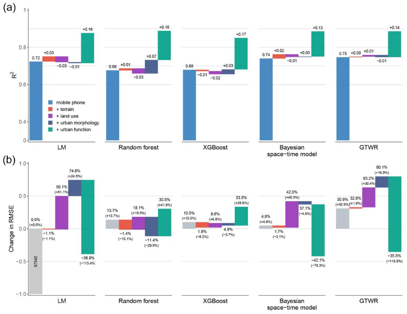
Model performance evaluation across different models and covariate combinations: (a) changes in absolute values of R² with incremental addition of covariates, (b) relative changes in RMSE compared with baseline model. Here the baseline model is the LM model containing only mobile phone positioning data. The R² and RMSE in this figure were calculated using data from 6 am to 11 pm for one day (July 13).

However, the RMSE changes differently when adding covariates among five models, as shown in Figure 1b. First, we found that the Bayesian space-time model yields the best performance than others when only using mobile phone positioning data as the covariate. Its RMSE of increased 4.8% compared with LM while other models increases more than 10.0%. However, the RMSE of the spatial statistical models show larger variations when adding more variables into the model. On the contrary, the RMSE of random forest and XGBoost are less sensitive to the additional variables. Finally, urban function data, which remarkably improves R² among the five models, exhibits distinct contributions to RMSE. It reduces RMSE in statistical models, particularly for the Bayesian space-time model (42.1% lower than baseline), but worsens the accuracy in machine learning models (>30% increase than baseline), which goes against the general knowledge in urban studies. Further evidence is provided in the following sections.

The contribution of covariates in dynamic population mapping

We compared the contributions of covariates in dynamic population mapping by taking the Bayesian space-time model and the random forest as examples, as they achieve the best performance in R² and RMSE among spatial statistical and machine learning models, respectively. To measure the contribution of the covariates, we adopted the posterior distribution of the coefficient of each covariate for the Bayesian space-time model (Figure 2a), and took the %IncMSE (percentage of the increase in mean-squared-error (MSE) of predictions) for the random forest (Figure 2b) respectively.

Figure 2.

The contributions of covariates across different models and covariate combinations. (a) The posterior distribution of covariates in the Bayesian space-time model. The space-time model took data for one day as input together, so there only exists one posterior distribution for each covariate from the model with a certain covariate combination. (b) The %IncMSE of covariates in the random forest model. The boxplots comprise values from models for each hour.

In Figure 2a, we found that mobile phone positioning data dominated the model when only terrain information was additionally added. It has a coefficient (mean 1.07) three times larger than the second covariate (slope, mean 0.33). Meanwhile, its relatively small standard deviation (SD) (0.006) induces a narrow posterior distribution. When later adding the land use and urban morphology data, the coefficient of mobile phone positioning declines to around 0.8 with wider confidence intervals (SD 0.017). At the same time, built-up land use and road density gain the only positive coefficient in the covariate of their respective types. Finally, when considering the urban function information, mobile phone positioning data present the flattest posterior distribution (SD 0.027) and share an almost equal coefficient (mean 0.43) with slope (mean 0.48), built-up land use (mean 0.42), and residential area (mean 0.40).

The importance of covariates in the random forest model follows a similar pattern to the Bayesian space-time model. For example, the importance of mobile phone positioning gradually declines as more covariates were subsequently added; residential, education, and commercial areas rank the top three in urban function data. However, we found that the importance of the residential area (%IncMSE 2.60) and education area (%IncMSE 1.03) overwhelmed the mobile phone positioning (%IncMSE 0.56) after they were finally added, which might disturb the detection of population dynamics. This phenomenon partially explains why the machine learning techniques return higher RMSE when introducing urban function data.

Influences of covariates on population distribution patterns

To investigate the influences of different covariates, we further describe how the population distribution changes when adding the covariate into the model, taking the Bayesian space-time population estimates at 9 pm as an example. The results are shown in Figure 3.

Figure 3.

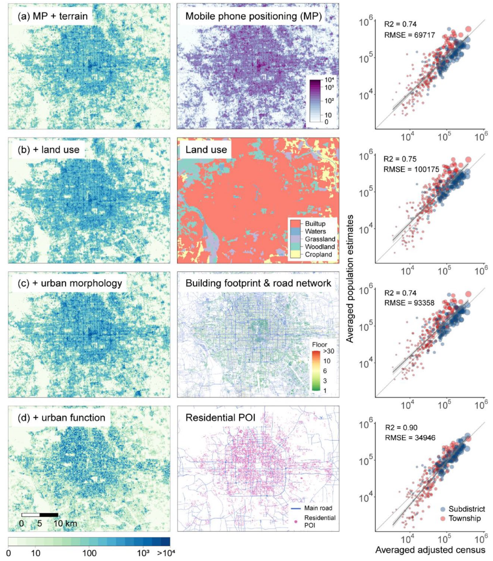
Changes in population distribution patterns with incremental addition of covariates. The left column represents the population distribution at 9 pm estimated by the Bayesian space-time model with different combinations of covariates (a) mobile phone positioning and terrain, (b) adding land use data, (c) adding urban morphology data, (d) adding urban function data. The middle column shows the most representative data in each type of covariates. The right column shows the estimation accuracy.

We found that in the case where covariates only contain mobile phone positioning and terrain, the spatial pattern of the population looks quite similar to mobile phone positioning data (Figure 3a), which mainly owes to its dominance, as revealed in Figure 2. When the land use data are subsequently added, the pattern in the urban center shows no apparent change but a higher value in general (Figure 3b), which is mainly contributed by the positive coefficient of built-up land use (Figure 2a). Meanwhile, the artificial-natural surface interface in the suburbs is much clearer. Woodlands, grasslands, croplands around the city, and waters inside the city have few people, implying the efficacy of land-use data in suppressing occurrent mobile phone positioning converting into population estimates. However, the higher RMSE when introducing land-use data across five models illustrates that this suppression is inconducive to improving the accuracy of population mapping, as revealed in Figure 1b.

When introducing the urban morphology data, population distribution starts to agglomerate along with the city topology (Figure 3c). The population on the built-up land use starts to be fragmentized again, where the population concentrates in high built-up density areas. In particular, the population along the city roads seems to be higher and more pronounced. Although a slightly lower RMSE is evidenced in the Bayesian space-time model, this pattern may be unreasonable to some extent since the population density along the road should not stand out too much than elsewhere at night. Considering the inconsistent impacts of urban morphology data on mapping accuracy, as shown in Figure 1, we recommend incorporating urban morphology information in large-scale (e.g., national or regional) population mapping but treating it with caution to the urban scale.

Finally, adding urban function data brings our night-time population estimates closest to population inhabitation (Figure 3d). The population distribution appears to be more uneven. Green spaces in the city center have few people, while the highest population density can be found in residential areas. Moreover, urban function data can suppress abnormal hotspots in mobile phone positioning data. For example, the mobile phone positioning at the center of our plot has a large area of peaks, which invariably leads to high population estimates. However, this is an area full of attractions and bungalows. Only by incorporating urban function data can the real situation of the lower population at that place at night be restored, which results in the highest R² and the lowest RMSE of the Bayesian space-time model in Figure 1.

Population dynamics over Beijing

Taking the optimal space-time model, we estimated hourly population distribution from 6 am to 11 pm for one week (July 12 to July 18). After averaging the results by the hour, we found clear differences between the population distribution during daytime and night-time (Figure 4ab). We then zoomed in on some typical areas that show great volumes of population variation to provide an intuitive view of the laws of population dynamics (Figure 4c). We found that their population distribution patterns in the morning (6:00–8:00) and at night (21:00–23:00) are similar, which is the opposite of the daytime (9:00–17:00). In particular, population variation patterns at 18:00–20:00 are not as obvious as in other periods, mainly owing to the larger-scale population movement at rush time. Furthermore, we found that residential area (A) shows distinct variation patterns than other functional areas, and its population is smaller in the daytime but larger in the early morning and evening. On the contrary, the areas where science and education (B), finance (C), and business (D) are concentrated show an inversed U-shape.

Figure 4.

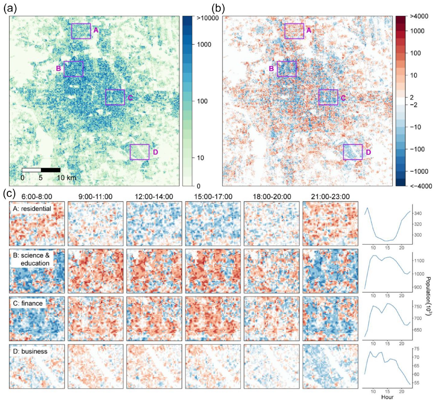
Spatial patterns of population dynamics. (a) One-week-averaged population distribution. (b) Difference between one-week-averaged distribution at 9–11 pm and subplot a. (c) Zoom-in plots for changes in population distribution in A. Huilongguan (residential area), B. Zhongguancun (science and education), C. Guomao (finance), and D. Kechuangqu (business). We calculated the population variation as the difference between the one-week-averaged population in each 3-hour bin and the overall one-week-averaged population. The subplot c shares the same color legend with subplot b. The line plots on the right show variations of total population count in zoom-in areas.

We subsequently extracted the population on different amenities using area-of-interests (AOI) shapefiles. After filtering out AOIs with areas less than 10,000 m² or an average population count of less than 100, we selected 3,988 residential areas, 2,303 leisure places (including green space and recreation), 531 commercial areas, and 321 transportation facilities, and 87 hospitals out of 17,234 records. We then standardized the population for each AOIs to eliminate dimensional effects and summarized them to obtain distributions of population count skewing from average. The results are presented in Figure 5.

Figure 5.

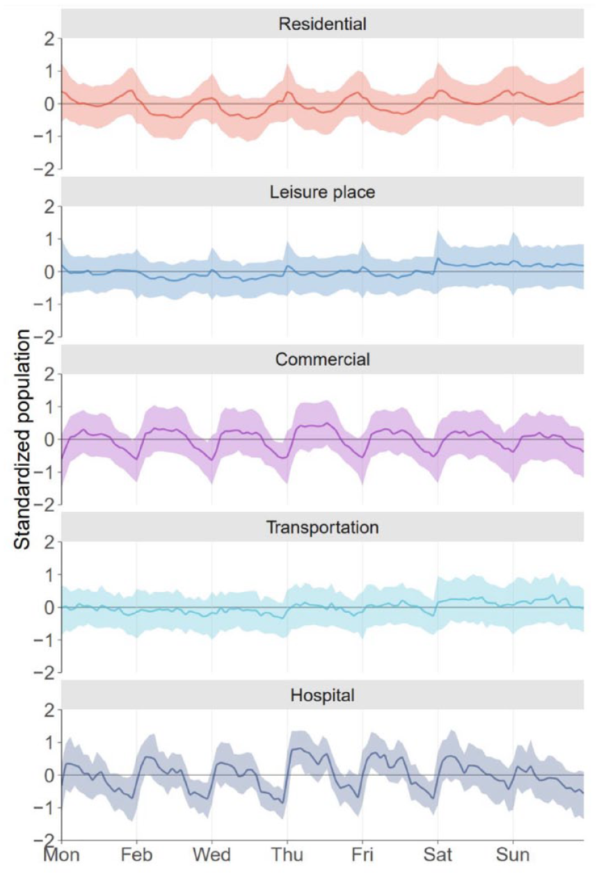
Population variation patterns across different amenities. This figure shows the hourly population from 6 am to 11 pm for one week. We extracted the population count on each AOI and then standardized them separately. The line in each subplot shows the mean value of the standardized population for each kind of amenity. The shadow area covers the 25% to 75% quantiles.

We found distinct visitation laws across different amenities. Residential areas have fewer people during the day while higher populations at night. In particular, they see more people on the weekends than weekdays. Commercial areas and hospitals show inverse fluctuations compared with residential areas. Although there is a short-term pullback at midday, most of them have higher population agglomeration in the daytime. At night, however, they are almost empty. The other two kinds of amenities show less dramatic changes. The population at leisure places sees no apparent change on weekdays but a consistent increase on weekends. Likewise, transportation facilities also hold a higher population over the weekend. The population dynamics in the latter two places jointly uncover the phenomenon that people went out for leisure on weekends.

Discussion and conclusion

Understanding population dynamics at fine spatiotemporal granularities is valuable to studies reliant on dynamic population distribution information. With the booming availability of auxiliary data, researchers tend to incorporate as many covariates as possible into the machine learning models to realize more accurate population estimation, readily believing that their strengths in detecting nonlinear relationships would help avoid the multicollinearity and overfitting problems in statistical models. However, there is still no empirical evidence on whether the machine learning technique is superior to traditional statistical or spatial statistical methods and whether more covariates always guarantee more accurate results.

This paper systematically evaluates the performance of commonly used spatial statistical and machine learning approaches in population dynamics modeling, using an example of Beijing’s inner-city hourly population mapping at 100m resolution. We found that the Bayesian space-time model performs best in dynamic population mapping when all the auxiliary data in this paper are available, implying that modeling spatiotemporal autocorrelation is the top priority when mapping high-frequency population dynamics. However, this conclusion can be drawn because adding urban function data lowers the estimation bias of statistical models but interferes with capturing population dynamics in machine learning techniques we used. In the absence of such covariates, random forest, or XGBoost methods could ensure more stable performance, although R² is hard to achieve the highest value.

Our conclusions are consistent with and complementary to previous studies on population mapping. For example, Wang et al. (2021) found that the Bayesian space-time model can help understand spatiotemporal variability of population dynamics using mobile phone positioning data, which favored the stability of estimated population distribution patterns and the reproduction of reasonable temporal fluctuation. Lwin et al. (2016) also highlighted the necessity of considering the temporal dependency of population distribution in urban areas, which could further support the prediction of population distribution (Chen et al., 2018). Meanwhile, Sinha et al. (2019) demonstrated that the random forest model is sensitive to spatial autocorrelation and spatial representation of the true population, which easily increased the variance of residuals in population downscaling mapping.

In terms of covariates contribution, we highlighted the importance of urban function data in urban population mapping, which also matches similar studies. For example, Yao et al. (2017) found that mobile phone positioning data ranked first in dynamics population mapping, followed by the density of life service, education, clinic, and residential facilities. Similar patterns could also be found in Stevens et al. (2015). Although data for health facilities were absent in our study, and the fact that building footprint accounted for more contributions in their building-level population mapping design, our result drew a consistent conclusion. Comparatively, covariates describing the basic underlying surface such as elevation and slope were less important. However, these conclusions mainly apply to population mapping research to an urban extent, especially in the absence of dramatic topographic relief because Beijing is a city with a flat center surrounded by mountains in the North and West. Despite the slope holding a comparable coefficient with other explanatory variables in the Bayesian space-time model, covariates of terrain were hard to influence spatial population patterns in the relatively flat city center (Figure 3). However, they may be more important in mountainous cities. Meanwhile, large-scale population mapping also requires them to act as a basic control (Lloyd et al., 2017, 2019).

We acknowledge that some limitations exist in our study. First, we adjusted the statistical population using mobile phone positioning data prior to the modeling procedure to realize dynamic population mapping. We assumed the mobile phone activity in each administrative unit is comparable over time. However, its heterogeneities across ages, regions, and land-use types make our assumption violate the reality. Second, we did not evaluate newly developed methods to explicitly distinguish the influence of different population distribution characteristics on mapping accuracy. For example, people have long been aware of the defects of applying random forest directly to spatial modeling due to their ignorance of geographic locations, thereby incentive the emergence of spatial extensions of random forest algorithms (Georganos et al., 2021; Hengl et al., 2018). Some state-of-art deep learning methods, such as convolutional neural network (CNN) and graph convolutional network (GCN), can also take spatiotemporal autocorrelation into account. More recently, ensemble methods that blend multiple approaches have also been developed to integrate the advantages of various methods, thereby achieving more accurate results (Gao et al., 2022). Third, we integrated the covariates most representative of population mapping studies available at 100 m resolution. However, we dropped some commonly used variables due to the coarse spatial resolution or data accessibility issues, such as night-time light remote sensing data (Chen et al., 2021; Li and Zhou, 2018). We admit that incorporating those missing covariates might influence the conclusion we drew. Fourth, we only modeled population dynamics on an hourly basis. Our conclusions on the model performance and covariates contributions might vary at different temporal scales. We recommend scholars carefully introduce our conclusions to studies with other spatiotemporal granularities. Fifth, our one case study in Beijing is unable to demonstrate the generality of our conclusions for other cities. Stronger evidence requires multiple dataset testing in different regions in future studies. Finally, our conclusions provide reference mainly for population mapping on the urban extent. In terms of large-scale population mapping research, the opposite might exist. For example, urban function data might be less important, while the unimpressive road density covariates in our study might account for more in mapping accuracy. Therefore, we recommend that researchers carefully choose modeling strategies and covariates suitable for different circumstances to map population dynamics with the least bias in future studies.

Our research provides empirical suggestions for other urban population mapping studies. On the one hand, we rejected the common prejudice that data-driven machine learning techniques always promise better results than traditional statistical methods. In contrast, explicitly introducing spatiotemporal dependencies would enhance the model interpretability and lower the estimation bias. On the other hand, we demonstrated the irreplaceable benefits of integrating information on urban functions, which helps understand the high-frequency population dynamics of different amenities within the city. Taking advantage of our findings, scholars can better design their modeling framework and improve dynamic population distribution mapping accuracy, thereby strengthening the rationale for revealing human activity patterns.

Footnotes

Author contribution

JW and CZ designed the project. JW and ZC collected and analyzed the data. JW, ZC and KZ interpreted the results. ZC, JW and KZ wrote the manuscript. JW, YG, and CZ supervised and edited the manuscript. All authors contributed to the development of the manuscript and approved the final version for publication.

Code availability

Codes used in this paper are available at .

Data availability

All data used in this paper are publicly available at . Beijing’s hourly population at 100 m resolution for 2015 is publicly available in the GitHub repository. The data for 2020 and the following years will be publicly accessible once it is finished.

Declaration of conflicting interests

The author(s) declared no potential conflicts of interest with respect to the research, authorship, and/or publication of this article.

Funding

The author(s) disclosed receipt of the following financial support for the research, authorship, and/or publication of this article: This research was funded by the National Natural Science Foundation of China (No. 41971409) and the Youth Innovation Promotion Association of the Chinese Academy of Sciences (No. 2020052). The funders had no role in study design, data collection and analysis, decision to publish, or preparation of the manuscript.

Author biographies

Zhifeng Cheng is a master’s student at the University of Chinese Academy of Sciences and the State Key Laboratory of Resources and Environmental Information System, Institute of Geographic Sciences and Natural Resources Research, Chinese Academy of Sciences (CAS). His research is now focused on mapping social-economic dynamics with big data.

Jianghao Wang is an associate professor at the State Key Laboratory of Resources and Environmental Information System, Institute of Geographic Sciences and Natural Resources Research, CAS. His research interests concentrate on spatiotemporal data mining.

Kaixin Zhu is a master’s student at the University of Chinese Academy of Sciences and the State Key Laboratory of Resources and Environmental Information System, Institute of Geographic Sciences and Natural Resources Research, CAS. His research is now focused on modeling human mobility using geospatial big data.

Yong Ge is currently a Professor at the State Key Laboratory of Resources and Environmental Information System, Institute of Geographic Sciences and Natural Resources Research, CAS. Her research is focused on spatiotemporal statistics.

Chenghu Zhou is currently a Professor at the State Key Laboratory of Resources and Environmental Information System, Institute of Geographic Sciences and Natural Resources Research, CAS. His research mainly focuses on geospatial big data mining.

References

Bagan

Yamagata

(2015) Analysis of urban growth and estimating population density using satellite images of nighttime lights and land-use and population data. GIScience and Remote Sensing 52(6): 765–780.

Bakka

Rue

Fuglstad

, et al. (2018) Spatial modeling with R-INLA: A review. Wiley Online Library. Available at: https://onlinelibrary.wiley.com/doi/abs/10.1002/wics.1443 (accessed 12 July 2022).

Belle

Wang

, et al. (2019) Impacts of snow and cloud covers on satellite-derived PM2.5 levels. Remote Sensing of the Environment 221: 665–674.

Blangiardo

Cameletti

Baio

, et al. (2013) Spatial and spatio-temporal models with R-INLA. Spatial and Spatio-temporal Epidemiology 7: 39–55.

Breiman (2001) Random forests. Machine Learning 45: 5–32.

Chen

, et al. (2021) A new method for building-level population estimation by integrating LiDAR, nighttime light, and POI data. Journal of Remote Sensing 2021: 803796.

Chen

Pei

Shaw

S-L

, et al. (2018) Fine-grained prediction of urban population using mobile phone location data. International Journal of Geographical Information Science 32(9): 1770–1786.

Chen

Guestrin

(2016) XGBoost: A scalable tree boosting system. arXiv [cs.LG]. Available at: http://arxiv.org/abs/1603.02754 (accessed 12 July 2022).

Chen

Zhang

, et al. (2019) Downscaling census data for gridded population mapping with geographically weighted area-to-point regression kriging. IEEE Access 7: 149132–149141.

10.

Cheng

Wang

(2022) Mapping monthly population distribution and variation at 1-km resolution across China. International Journal of Geographical Information Science 36(6): 1166–1184.

11.

Deville

Linard

Martin

, et al. (2014) Dynamic population mapping using mobile phone data. Proceedings of the National Academy of Sciences 111(45): 15888–15893.

12.

Fotheringham

Crespo

Yao

(2015) Geographical and temporal weighted regression (GTWR). Geographical Analysis 47(4): 431–452.

13.

Gao

, et al. (2022) Improving the accuracy of extant gridded population maps using multisource map fusion. GIScience & Remote Sensing 59(1): 54–70.

14.

Gaughan

Stevens

Huang

, et al. (2016) Spatiotemporal patterns of population in mainland China, 1990 to 2010. Scientific Data 3: 160005.

15.

Georganos

Grippa

Niang Gadiaga

, et al. (2021) Geographical random forests: a spatial extension of the random forest algorithm to address spatial heterogeneity in remote sensing and population modelling. Geocarto International 36(2): 121–136.

16.

Hengl

Mendes de Jesus

Heuvelink

GBM

, et al. (2017) SoilGrids250m: Global gridded soil information based on machine learning. PloS One 12(2): e0169748.

17.

Hengl

Nussbaum

Wright

, et al. (2018) Random forest as a generic framework for predictive modeling of spatial and spatio-temporal variables. PeerJ 6: e5518.

18.

Klopp

Petretta

(2017) The urban sustainable development goal: Indicators, complexity and the politics of measuring cities. Cities 63: 92–97.

19.

Leasure

Jochem

Weber

, et al. (2020) National population mapping from sparse survey data: A hierarchical Bayesian modeling framework to account for uncertainty. Proceedings of the National Academy of Sciences 117(39): 24173–24179.

20.

Leyk

Gaughan

Adamo

, et al. (2019) The spatial allocation of population: a review of large-scale gridded population data products and their fitness for use. Earth System Science Data 11: 1385–1409.

21.

Zhou

(2018) Dasymetric mapping of urban population in China based on radiance corrected DMSP-OLS nighttime light and land cover data. The Science of the Total Environment 643: 1248–1256.

22.

Liu

Huang

, et al. (2021) Characterizing the complex influence of the urban built environment on the dynamic population distribution of Shenzhen, China, using geographically and temporally weighted regression. Environment and Planning. B, Urban Analytics and City Science 48(6): 1445–1462.

23.

Lloyd

Sorichetta

Tatem

(2017) High resolution global gridded data for use in population studies. Scientific Data 4: 170001.

24.

Lloyd

Chamberlain

Kerr

, et al. (2019) Global spatio-temporally harmonised datasets for producing high-resolution gridded population distribution datasets. Big Earth Data 3(2): 108–139.

25.

Lwin

Sugiura

Zettsu

(2016) Space–time multiple regression model for grid-based population estimation in urban areas. International Journal of Geographical Information Science 30(8): 1579–1593.

26.

Panczak

Charles-Edwards

Corcoran

(2020) Estimating temporary populations: a systematic review of the empirical literature. Humanities and Social Sciences Communications 6: 87.

27.

Patel

Stevens

Huang

, et al. (2017) Improving Large Area Population Mapping Using Geotweet Densities. Transactions in GIS 21(2): 317–331.

28.

Samuel-Rosa

Heuvelink

GBM

Vasques

, et al. (2015) Do more detailed environmental covariates deliver more accurate soil maps? Geoderma 243–244: 214–227.

29.

Sinha

Gaughan

Stevens

, et al. (2019) Assessing the spatial sensitivity of a random forest model: Application in gridded population modeling. Computers, Environment and Urban Systems 75: 132–145.

30.

Smith

Bates

Wing

, et al. (2019) New estimates of flood exposure in developing countries using high-resolution population data. Nature Communications 10: 1814.

31.

Song

Feng

Xia

, et al. (2021) Impacts of changing urban land-use structure on sustainable city growth in China: A population-density dynamics perspective. Habitat International 107: 102296.

32.

Stevens

Gaughan

Linard

, et al. (2015) Disaggregating census data for population mapping using random forests with remotely-sensed and ancillary data. PloS One 10(2): e0107042.

33.

Tatem

Adamo

Bharti

, et al. (2012) Mapping populations at risk: improving spatial demographic data for infectious disease modeling and metric derivation. Population Health Metrics 10(8).

34.

Liu

, et al. (2022) An ensemble method to generate high-resolution gridded population data for China from digital footprint and ancillary geospatial data. International Journal of Applied Earth Observation and Geoinformation 107: 102709.

35.

Wang

Zhou

, et al. (2018) Mapping population density in China between 1990 and 2010 using remote sensing. Remote Sensing of Environment 210: 269–281.

36.

Wang

Yue

, et al. (2021) A Bayesian spatio-temporal model to analyzing the stability of patterns of population distribution in an urban space using mobile phone data. International Journal of Geographical Information Science 35(1): 116-134.

37.

Wardrop

Jochem

Bird

, et al. (2018) Spatially disaggregated population estimates in the absence of national population and housing census data. Proceedings of the National Academy of Sciences 115(14): 3529–3537.

38.

World Bank (2020) Urban Development. Available at: www.worldbank.org/en/topic/urbandevelopment/overview (accessed 12 July 2022)

39.

Yao

Liu

, et al. (2017) Mapping fine-scale population distributions at the building level by integrating multisource geospatial big data. International Journal of Geographical Information Science 31(6): 1220–1244.

40.

Zhao

Yang

, et al. (2019) Improved population mapping for China using remotely sensed and points-of-interest data within a random forests model. The Science of the Total Environment 658: 936–946.

41.

Zhao

Zhou

Chen

, et al. (2021) Mapping hourly population dynamics using remotely sensed and geospatial data: a case study in Beijing, China. GIScience and Remote Sensing 58(5): 717–732.

42.

Zhao

Xia

, et al. (2021) Mapping Population Distribution Based on XGBoost Using Multisource Data. IEEE Journal of Selected Topics in Applied Earth Observations and Remote Sensing 14: 11567–11580.

Evaluating spatial statistical and machine learning models in urban dynamic population mapping

Abstract

Keywords

Introduction

Data

Census

Mobile phone positioning data

Terrain

Land use

Road network

Building footprints

Point-of-interest

Methods

The general framework of dynamic population mapping

Adjust census data

Evaluate the contribution of covariates

Population mapping models

Linear regression model

Geographically and temporally weighted regression

Bayesian space-time model

Random forest

eXtreme Gradient Boosting (XGBoost)

Model performance assessment

Results

Evaluate the model performance

The contribution of covariates in dynamic population mapping

Influences of covariates on population distribution patterns

Population dynamics over Beijing

Discussion and conclusion

Footnotes

Author contribution

Code availability

Data availability

Declaration of conflicting interests

Funding

Author biographies

References