
Abstract
Using a dynamic spatial panel model applied to 377 US Metropolitan Statistical Areas (MSAs), estimated over the period 2011-2021, significant differences are found between large MSAs regarding the relationship between labour productivity and economic mass, as measured by GDP. The methodology adopted illustrates the state of the art for spatial econometric modeling as it is often needed in practice, allowing for multiple endogenous regressors and dynamic effects. The estimation method applies synthetic instruments designed to limit negative effects of instrument overabundance.
Keywords
Introduction
This paper develops a methodology for analyzing productivity variation across cities and regions in the context of limited data availability and pervasive endogeneity. Informal data analysis shows that there are differences in economic performance as measured by productivity across Metropolitan Statistical Areas 1 (MSAs) and more formal modelling via dynamic spatial panel data models provides a more detailed and precise analysis than the signals provided by the initial informal analysis.
A distinctive contribution in the paper is a method that, rather than a single elasticity, allows the heterogeneity of productivity elasticities across cities and regions to be estimated. Based on GDP and employment data, this paper explores the productivity trends in the post-crisis era 2011 to 2021 for 377 MSAs and in particular for the 8 largest MSAs of the USA. These are the MSAs with employment greater than the 0.98 quantile of the employment distribution in 2001, amounting to 8 MSAs, namely those centered on Boston, Chicago, Dallas, Houston, Los Angeles, New York, Philadelphia and Washington. 2 We refer to these throughout as the top 8 MSAs. The approach adopted could in principle extend to other MSAs, but in the interest of practicality and ease of demonstration the number is purposefully kept low.
The analysis focusses on the effect of output, measured by GDP, on labour productivity, measured by the ratio of GDP to employment. This focus is chosen because persistent welfare inequalities between cities evidently depend on variations in productivity. Estimation is based on a dynamic spatial panel data model using a standard GMM estimator. Attention is paid to the possibility of endogeneity bias in parameter estimates, the possibility of nonstationarity of estimates, and issues caused by an overabundance of instrumental variables. In particular the paper highlights the application of synthetic instrumental variables as advocated by Fingleton (2023) in dynamic spatial panel data modelling, which helps to put estimation and inference on a more secure basis. This is because synthetic instruments can help reduce problems caused by a large number of instrumental variables, such as biased standard errors and unreliable diagnostic tests of model validity. Most notably, the standard test of overidentification, the Sargan-Hansen J test, can be unreliable. The paper provides estimates of short and long-run elasticities, that take account of spillover across space and time.
Theoretical Basis
There are several theoretical approaches that could be adopted to establish an equation that is the basis for empirical analysis, and although each commences with different assumptions, ultimately we do seem to have a case of equifinality, whereby each theory results in the same, or a very similar estimating equation in which productivity is a partial function of economic mass or some equivalent, and typically there is evidence of increasing returns to scale. Some alternatives are summarized in the Appendix. Here the focus is on the approach of Fingleton et al. (2023), in which the starting point is a fundamental equation that establishes a connection between a city’s output level and its economic mass. Representing the output level at time t in city i by Q
it
, and approximating the economic mass in city i at time t by its level of employment (L
it
), this fundamental equation asserts that an increase in economic mass, and hence variety of inputs (Fujita, Krugman, and Venables 1999; Jacobs 1969), which can be perceived as the city’s productive capacity, leads to a rise in production. It is crucial to note that this relationship exhibits nonlinearity. In fact, an increase in economic mass may generate more than a proportionate increase in production, so that a 1 percent increase in mass could potentially yield a production increase surpassing 1 percent. Increasing returns to scale are encapsulated in equation

Equation (1) does not explicitly incorporate productivity, but we can introduce it by taking logarithms and reorganizing the equation so that the logarithm of productivity level, ln P
it
appears as the left-hand side variable, hence

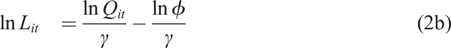


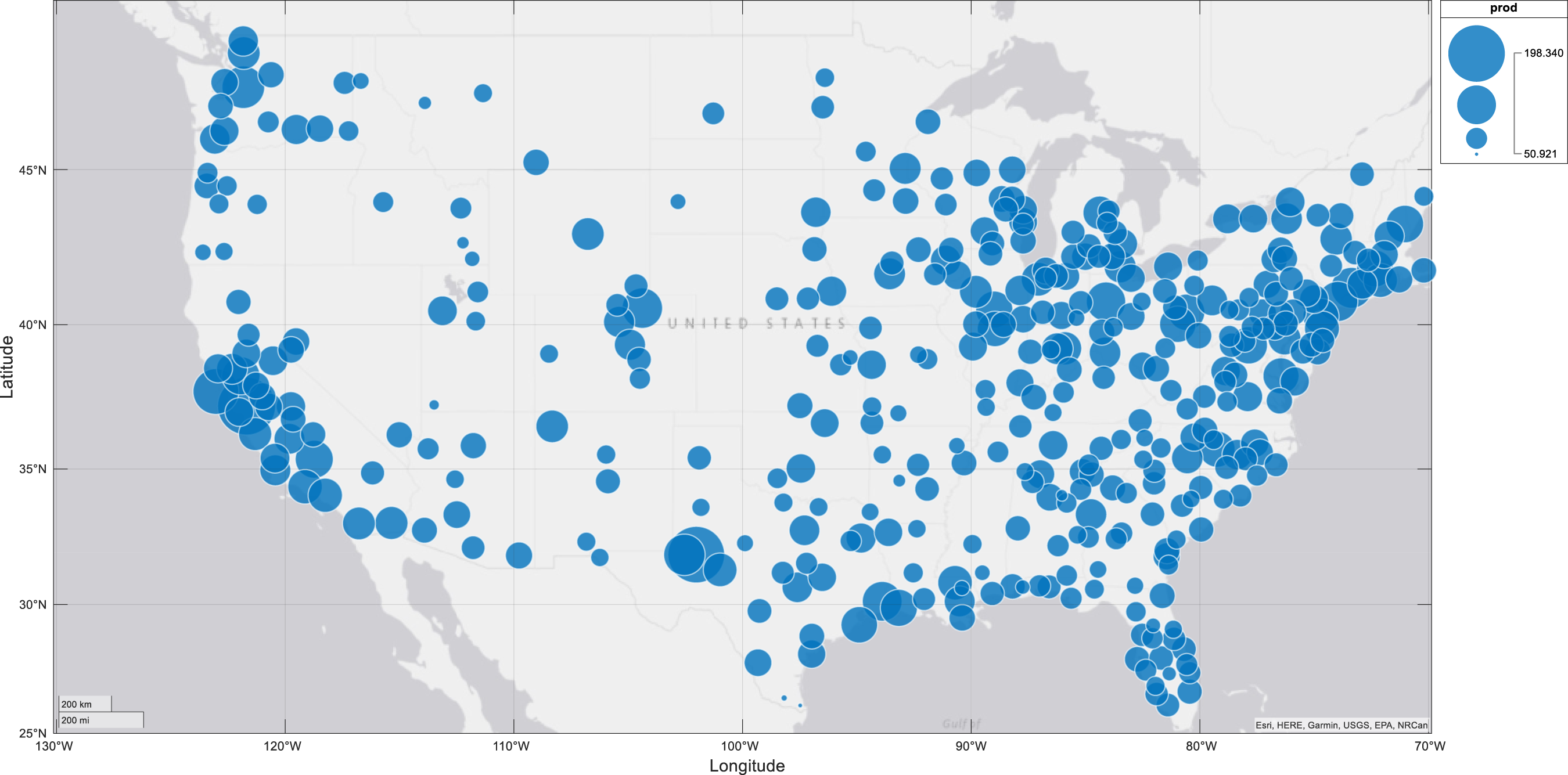
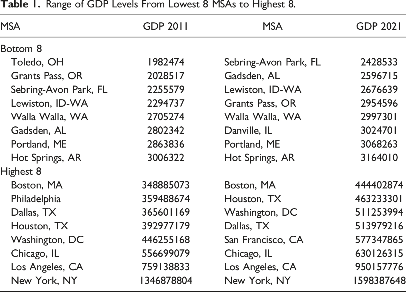
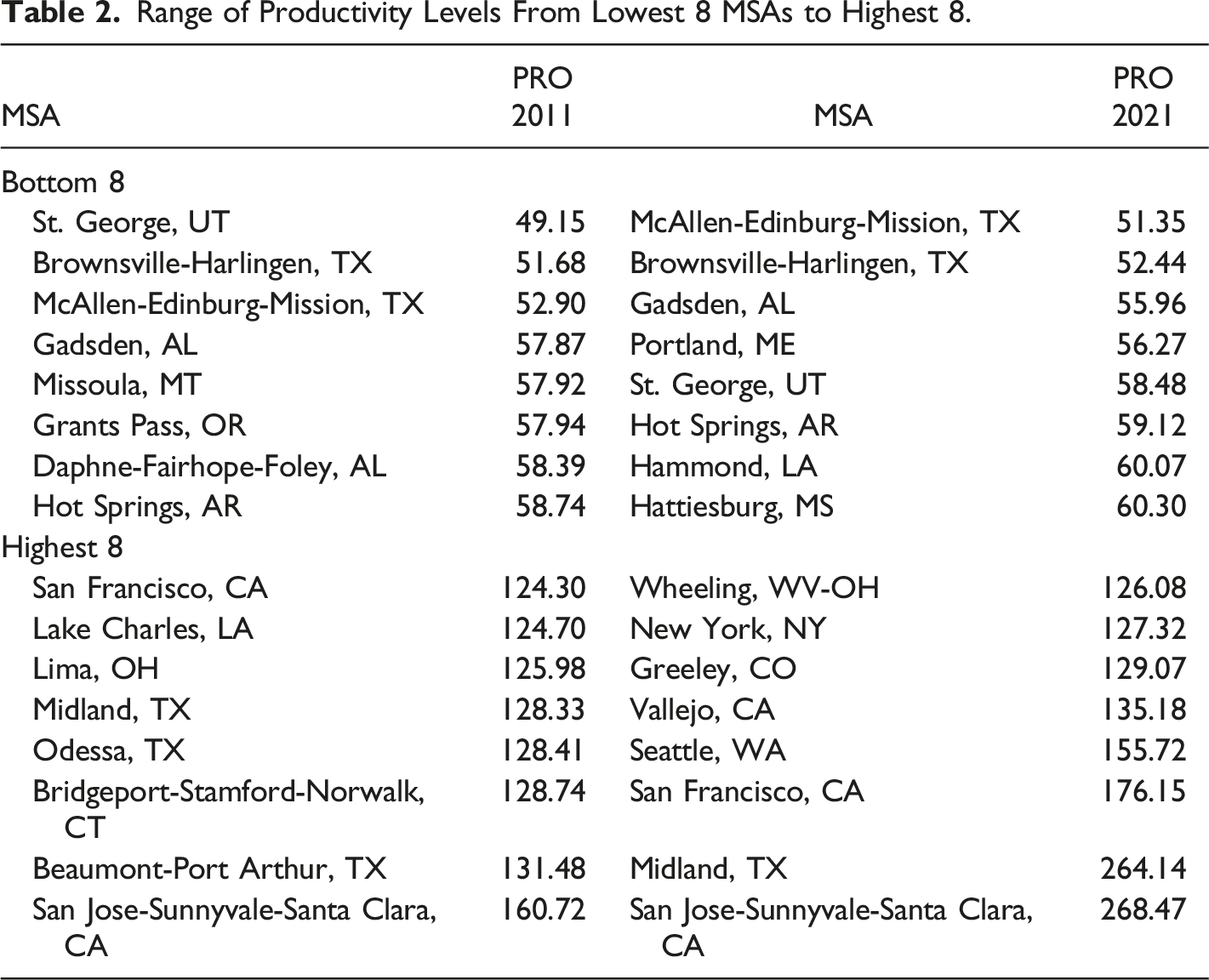
It is evident that when γ > = 1, indicating constant or increasing returns to scale, 1 > b = γ − 1/γ > = 0, and as γ approaches infinity, b approaches 1.0. Therefore, a positive value of b, which is less than 1.0, indicates increasing output causing increasing productivity. With 0 < = γ < 1, a 1 percent increase in labour causes a less than 1 percent increase in output, so we have diminishing returns for output with respect to labour, and falling productivity with respect to output, as indicated by b < 0. The basic theory, summarised by equations (1) through to (2e) is that higher output enhances externalities associated with economic mass, causing higher levels of productivity, and higher productivity is associated with higher wage levels and higher returns on other factors and possibly increases over a range of other indicators of social and economic well-being. As noted by Fingleton et al. (2023), ‘a large spatial economic mass not only provides the diversity and variety of inputs needed for production, and large ‘home’ (local) market opportunities for new enterprises (Jacobs 1969), but also a concentration of other assets that aid local businesses, such as hard and soft infrastructures, educational centres, skilled labour, institutional networks, and public and private research centres’. The large economic mass typical of the top 8 MSAs means that they in particular should have more extensive externalities deriving from the additional diversity and variety of inputs available for production in large cities, causing increasing returns to scale. A circular relationship between economic mass and productivity means that economic mass is best treated as endogenous, and this assumption is fundamental to the econometric methods adopted. Figures 1 and 2 provide an initial glimpse of the data, taken from the Bureau of Economic Analysis, as updated on December 8, 2022 to included new statistics for 2021 and revised statistics for 2017-2020. These data comprise GDP and employment levels for the years 2011 to 2021. Figure 1 shows that the level of output varies quite dramatically from the high point of New York, with Chicago, Miami, Los Angeles and San Francisco also very prominent, Figure 2 shows a much less dramatic variation in mean productivity level across cities, but with mean productivity about 4 times greater from highest MSA to lowest, some MSAs are possibly less productive than they could be. Increasing productivity can be a source of increasing output without the costs otherwise associated with additional inputs, such as additional labor, so that the economy as a whole produces more goods and services for the same amount of work. So for the US economy as a whole, raising productivity among lagging MSAs can have a beneficial effect on material welfare. Productivity is a critical source of prosperity. Notice however that Figures 1 and 2 do not show a clear-cut relationship between GDP and productivity, as evidenced also by the data, from the same source, in Tables 1 and 2. Clearly there are additional factors to take into account in trying to explain productivity variation across MSAs. Likewise, there are numerous papers taking various approaches to understanding US regional and urban productivity variation, and to cite just a few, see for example Moomaw (1983), Gerking (1993), Burger and Meijers (2010), Melo et al. (2017), Parilla and Muro (2017), and Caliendo et al. (2018). Mean GDP 2011-2021 across MSAs. Mean productivity 2011-2021 across MSAs. Range of GDP Levels From Lowest 8 MSAs to Highest 8. Range of Productivity Levels From Lowest 8 MSAs to Highest 8.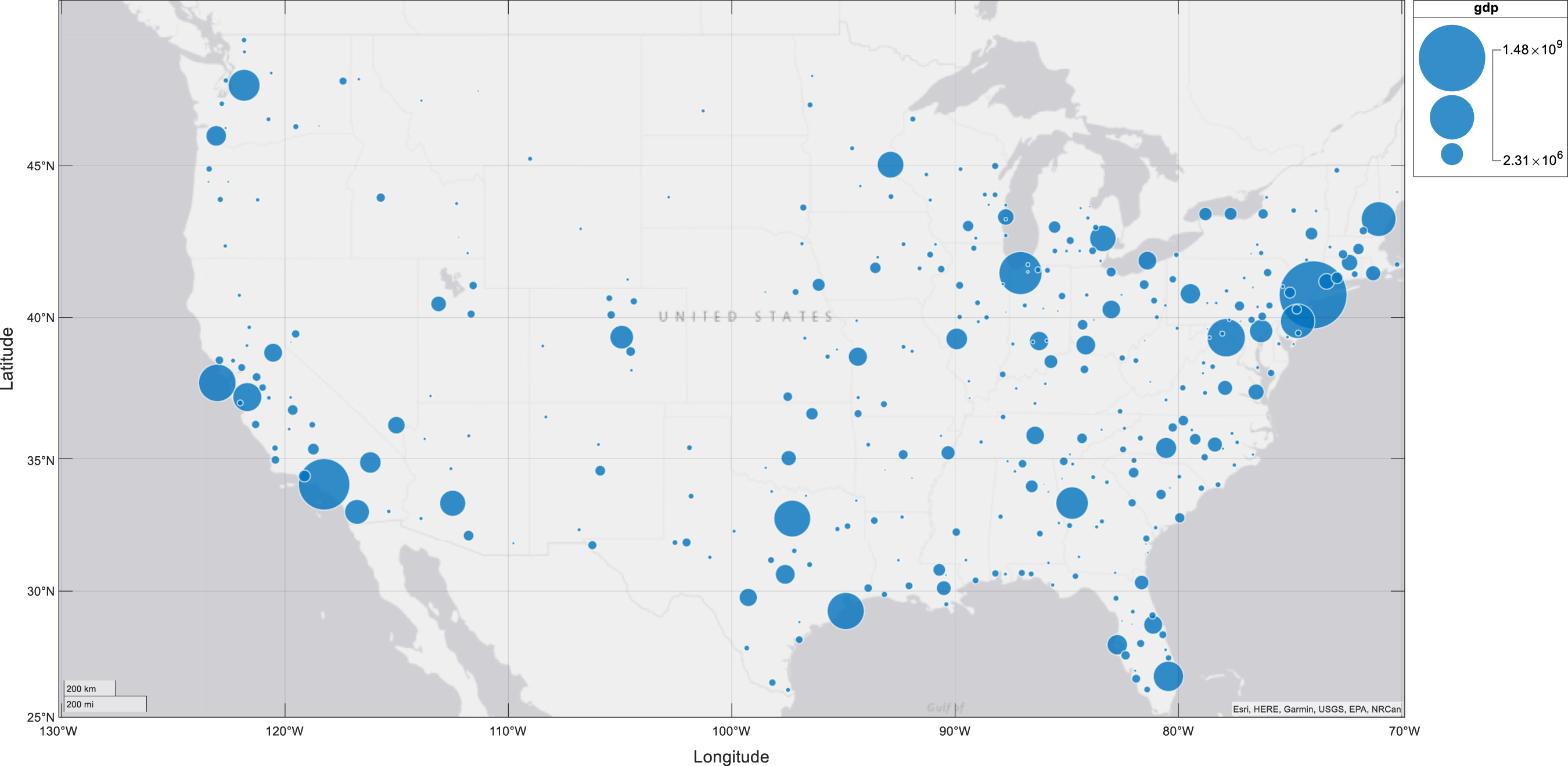
Introducing Spillovers
As possibly suggested by Figure 2, productivity in city 
In equation (3), ς
i
refers to a time-constant (n by 1) vector, and assuming that T is a large number, and |δ| < 1, then equation (3) converges to
Various designations of W are possible, but in this paper the W matrix is given by
In which d
ij
is the straight line distance between MSAs i and j, and ψ = max(eig) is the maximum eigenvalue of
To obtain spatial lags, we first introduce spatial dependence by multiplying equation (3) by the (n by n) matrix ρW to give
Subtracting equation (5) from equation (3) gives


Spillovers are across space are likely to occur because MSA boundaries are permeable; labour quality, various other socio-economic attributes, capital, ownership and management structures, supply-chain effects, spillovers of technology, etcetera, and consequently productivity, in ‘nearby’ MSAs are likely to affect, and be affected by, productivity in MSA i.
The Model
The fundamental theory relating productivity to output is encapsulated by equation (2e), while equation (8) expresses how productivity is related to productivity across space and time. These two fundamental causes of productivity variation are combined in equation (9) which is the result of adding a + β1 ln Q
t
to equation (8) in accordance with equation (2e). In addition the equation assumes that productivity is affected by variations in capital stock K
t
and human capital H
t
across MSAs, since these feature widely in many accounts of the causes of productivity variation, for example Mankiw, Romer, and Weil (1992), Becker (1993), Barro and Lee (2013), Ciccone and Peri (2006), and the World Bank (2019), to mention just a few. Notice however that spatial lags of regressors such as W ln Q
t
, W ln K
t
and W ln H
t
are not included in equation (9) because they do not follow directly from theory.
In equation (9) we have ln P
t
as a function of the spatial lag, the temporal lag and the spatial lag of the temporal lag. Regarding the variables K
t
and H
t
, we do not have explicit measures but nonetheless attempt to capture their effects in estimation. The term 
Equation (10) is obtained by taking first differences of equation (9). Section 5 outlines the rationale for estimating a model similar to equations (9) and (10).
Further Preliminary Insights
Using Bureau of Economic Analysis data described above, taking averages across 377 cities, log GDP 4 rises each year from 16.4203 in 2011 to 16.5668 in 2021, with the exception of 2020 when GDP is below its 2019 level. To look at trends in output disparities across cities, we use the coefficient of variation, which is the standard deviation divided by the mean so as to obtain a scale invariant measure. The coefficient of variation of log GDP rises inexorably each year from 0.0719 in 2011 to 0.0740 in 2021. With regard to employment, a similar picture emerges for mean log employment 5 averaging over the 377 cities, which increases each year from 12.0594 in 2011 to 12.1591 in 2021, with the exception of a dip in 2020. The coefficient of variation for log employment also rises each year from 0.0912 in 2011 to 0.0937 in 2021. Overall it appears that there is consistent post-crisis growth in output and employment with the exception of a COVID inspired slump in 2020, but the increasing coefficients of variation through time suggest widening differences between cities. This suggests that over the 2011-2021 period, urban economies experienced varying rates of recovery from the 2008 economic crisis and differing reactions to the shock of the COVID pandemic.
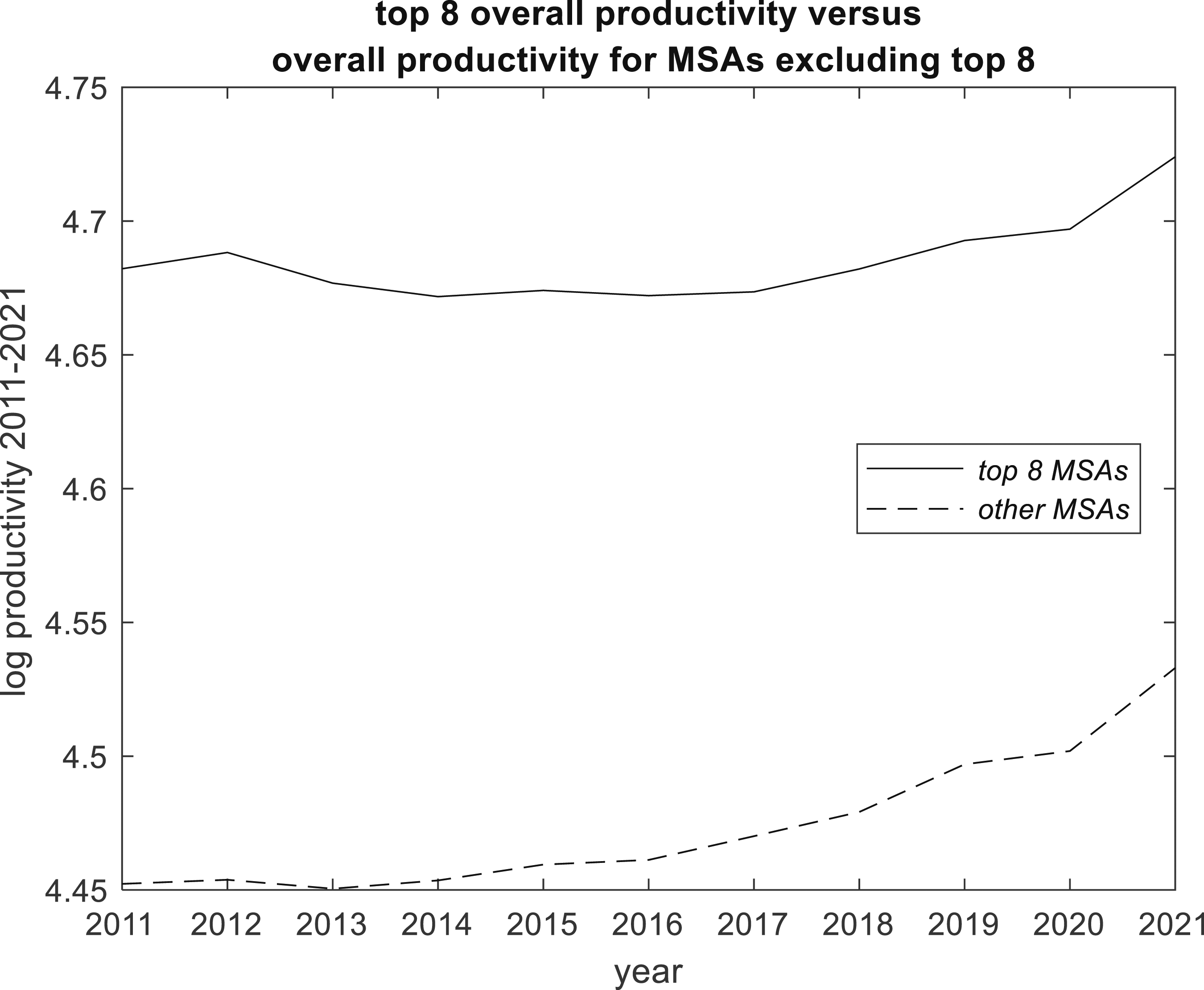
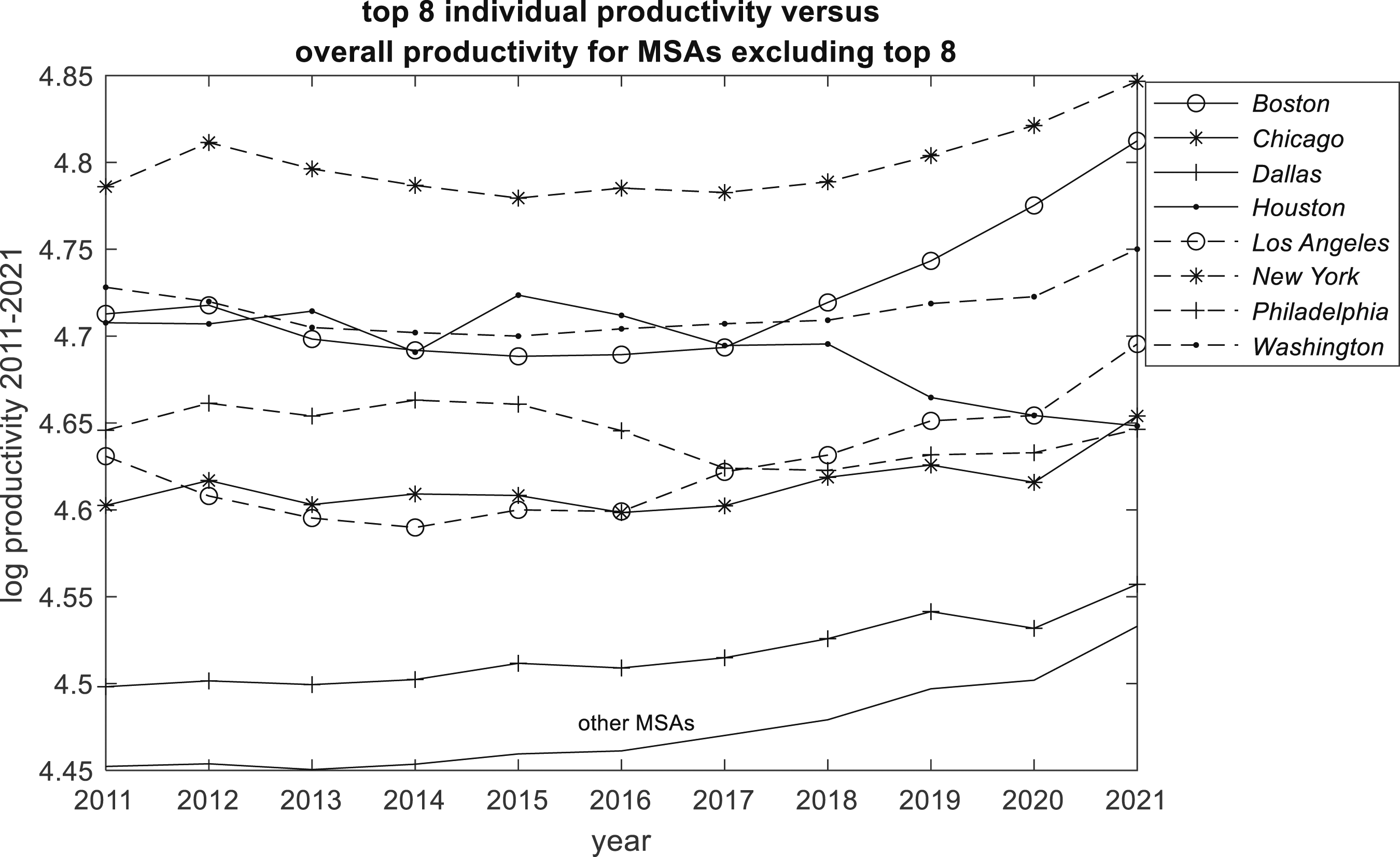
Figure 3, by focussing on a particular year and by taking logs, gives some insight into the otherwise somewhat concealed nexus between output and productivity. Figure 3 shows the relationship between log level of productivity and log level of GDP in 2011 for all 377 MSAs, indicating a strong positive correlation. Figure 4 emphasizes this by the path of log productivity (total GDP divided by total employment) for the top 8 MSAs versus the path for the smaller MSAs over the 2011-2021 period. Taken as a group, top 8 productivity is always higher than smaller MSA productivity. Overall we see that productivity was higher in 2021 than in 2011, but the path for the top 8 MSAs indicates no growth from 2012 to 2017, whereas the smaller MSAs show fairly consistent growth from 2013. For both MSA groups, the effect of the 2019 COVID pandemic is evident from the levelling off of productivity growth 2019 and 2020, with a sharp upturn from 2020. So the evidence is that while there were similarities between the MSA groups, the are also differences. One reason for the relatively muted growth of productivity for the top 8 MSAs as a group is the diverse within-group performance, as is evident in Figure 5. MSA Output versus Productivity in 2011. Productivity trends : Top 8 group compared with other MSAs. Productivity trends : Top 8 individuals compared with other MSAs.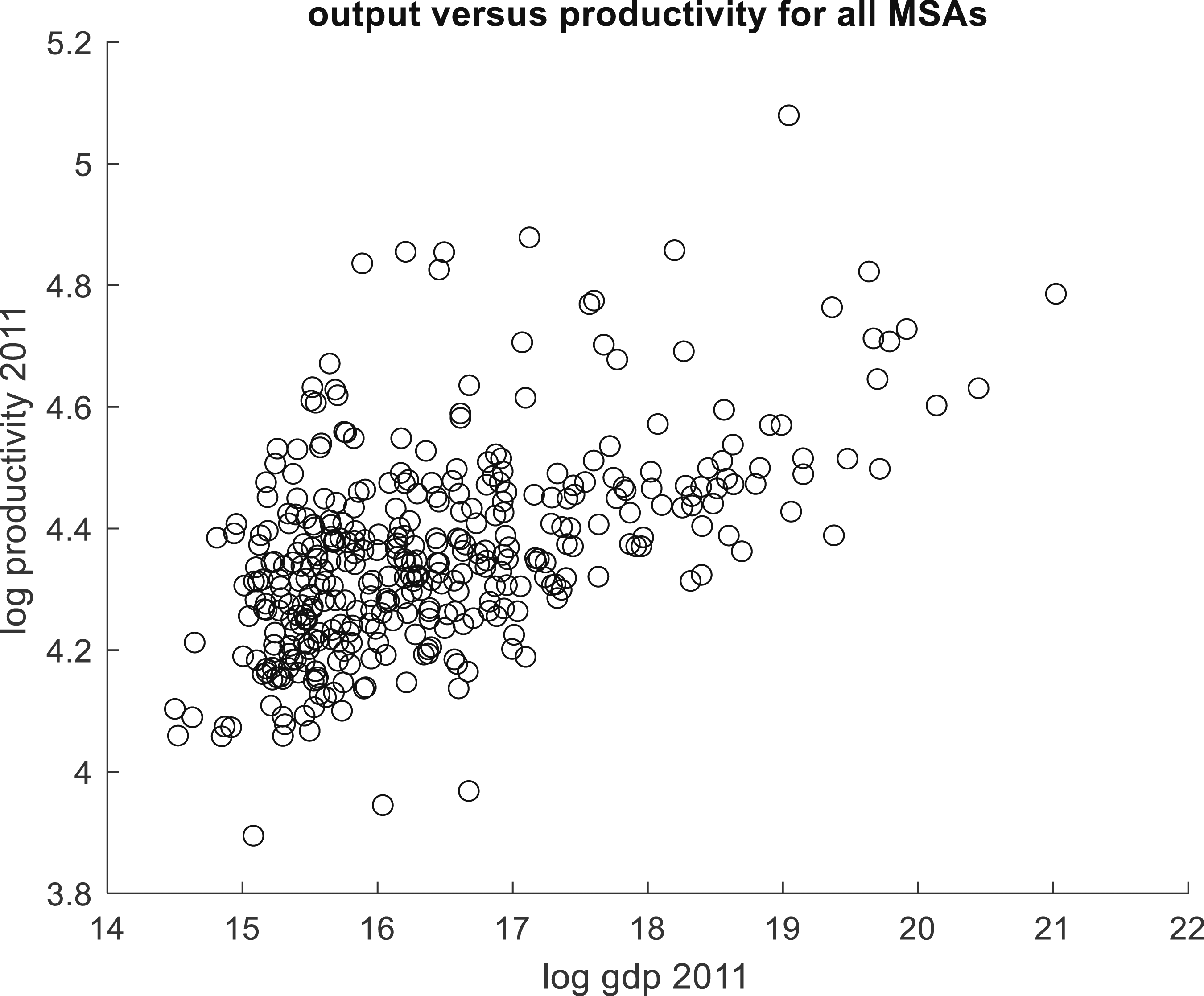
Econometric Analysis
Estimation
Our estimator, equation (12) is in terms of differences in logs, or exponential growth rates, and this helps us cope with an immediate problem in trying to estimate equation (9), which is lack of data. Clearly it would be ideal to include the level of capital stock in each MSA and for each year among the set of explanatory variables. However capital stock data at the subregional level are rarely if ever available, but as suggested in relation to equation (33), it is possible to assume that physical capital growth is proportionate to the rate of growth of output. According to Fingleton and McCombie (1958), ‘it is a stylized fact that for the advanced countries the capital stock grows either at approximately the same rate as output or slightly slower, and this assumption is applied in an analysis of productivity growth across European Union regions. McCombie and Thirlwall (1994, p.557) found that regressing capital growth on output growth for a sample of advanced countries, gave a slope coefficient that was not significantly different from unity’. Likewise, the author finds that a simple linear OLS regression of log US capital stocks 6 on log real GDP 7 gives a slope coefficient of b2 = 0.9051, R2 = 0.998. As McCombie and Roberts (2007) observe, ignoring the effect of capital accumulation on the growth of productivity is permissible if the capital-output ratio does not display any growth. 8 Accordingly we assume that, for MSA i, ln K it = b2 ln Q it . Bernat (1996) found a large impact on a state’s productivity growth by the productivity growth of the surrounding states, and McCombie and Roberts (2007) suggest that this could reflect a misspecification problem. Bernat (1996) did not include the growth of the capital stock [in the Verdoorn law] and “to the extent that this is not perfectly correlated with output growth, this will affect the error term”. In fact MSA output growth over 2011 to 2021 is also significantly spatially correlated. Based on W defined by equation (4), Moran’s I M = 0.0795, with expected value under the null hypothesis E(I M ) = −0.0027 and with var(I M ) = 2.4656e−5 under the randomization assumption, Z =(I M − E(I M ))/var(I M )0.5 = 16.55, which is very significantly different from 0 when referred to the N(0,1) distribution. One would anticipate that omitted capital stock growth would be correlated with spatially correlated output growth, and it is possible that the error induced by the omission of capital stock is spatially correlated, and the presence of the spatial lag in the model, which turns out to be highly significant, may to some extent be correcting for this mispecification.
Lack of human capital data presents a similar problem. Ciccone and Hall (1996) use cross-sectional data at State level and at county level, but a problem arises finding credible MSA-specific educational attainment time series. Some series are available from the American Community Survey (ACS), but there are omissions across time and space, measurement errors, and a mismatch between ACS MSAs and MSAs in this study. Alternatively, we consider the number of high school graduates (including equivalents) and the number of bachelors degrees and find that these indicators at the national (USA) level are both closely correlated with national (metropolitan portion) real GDP levels. Regressing log high school graduates on log real GDP for 2011 to 2021 gives R2 = 0.84. Regressing log bachelors’ degrees on log real GDP for 2011 to 2021 gives R2 = 0.97. Using a much longer series, a simple linear OLS regression of log Index of Human Capital per Person for the United States,
9
based on years of schooling and returns to education, on log real GDP gives b3 = 0.18539, R2 = 0.9619. We therefore assume that, for MSA i, ln H
it
= b3 ln Q
it
. So we get around the problem of lack of data for physical and human capital by attempting to capture their effects via their relationship with Q
t
. In equation (9), the term β1 ln Q
t
+ β2 ln K
t
+ β3 ln H
t
can be replaced by β1 ln Q
t
+ β2b2 ln Q
t
+ β3b3 ln Q
t
, and therefore the elasticity of P
t
with respect to Q
t
, broadly defined, can be represented as 
Equation (11) also includes the terms 
Sample of Data.
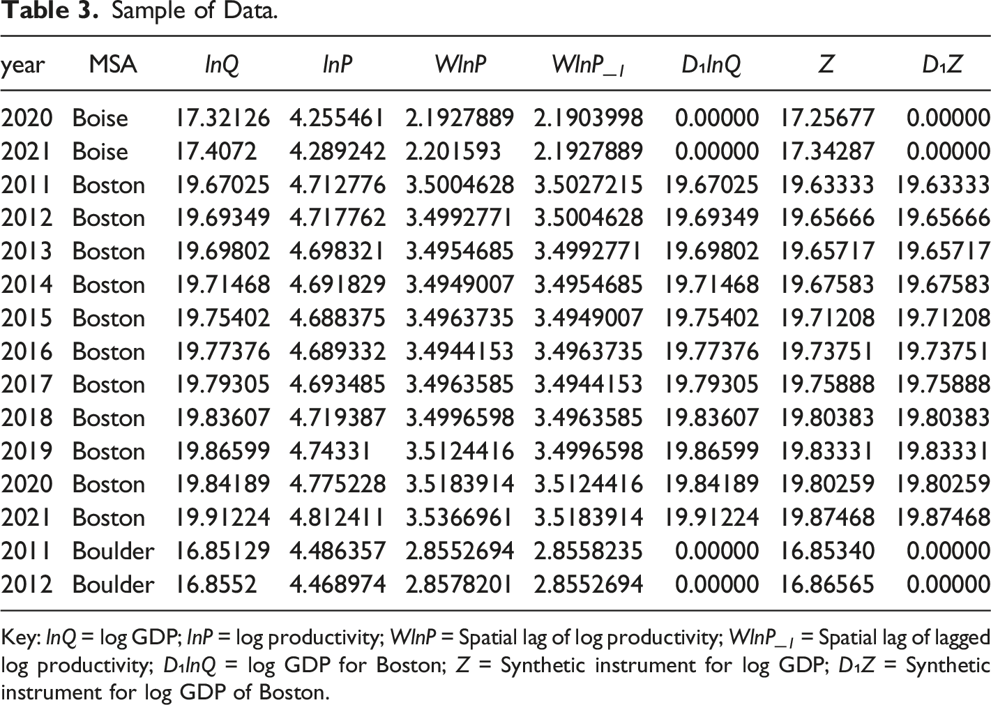
Key: lnQ = log GDP; lnP = log productivity; WlnP = Spatial lag of log productivity; WlnP_1 = Spatial lag of lagged log productivity; D₁lnQ = log GDP for Boston; Z = Synthetic instrument for log GDP; D₁Z = Synthetic instrument for log GDP of Boston.
Given that endogenous variables are contemporaneously related to the errors, there needs to be a careful choice of instruments in order to satisfy moments equations. An important prerequisite is that there is no serial correlation in the errors, in which case lags of the regressors can legitimately act as instrumental variables and satisfy orthogonality of the instruments and the differenced errors. For example, some moments conditions are

Instruments created in this way are referred to as GMM instruments, or HENR instruments (after Holtz-Eakin, Newey and Rosin 1988), with one instrument per variable, time period and lag distance amounting to (T − 2)(T − 1)/2 instruments for each endogenous variable. It is apparent that creating instruments in this way is rather expensive, since GMM instruments lead to quadratic growth in the number of instruments with respect to T. Instrument overabundance can have a detrimental effect on inference. For instance the estimated asymptotic standard errors of the efficient, two-step, GMM estimator are downwardly biased in small samples (Windmeijer 2005). 11 Additionally, Sargan–Hansen’s J test (Sargan 1958; Hansen 1982), which tests the null hypothesis of joint validity of the moments conditions under overidentification 12 can be greatly weakened by instrument proliferation (Andersen and Sørenson 1996; Bowsher 2002; Roodman 2009a, 2009b).
One solution to the problem of instrument overabundance is to collapse the instrument set over time, so that there is only one instrument for each variable and lag distance, giving (T − 2) instruments per endogenous variable. One can further limit the number of (collapsed) instruments by dropping instruments and reducing the lags 13 used to provide instruments from 2 to less than the maximum of T − 1. However with numerous endogenous variables requiring instruments, the number can still mount up and compromise estimation.
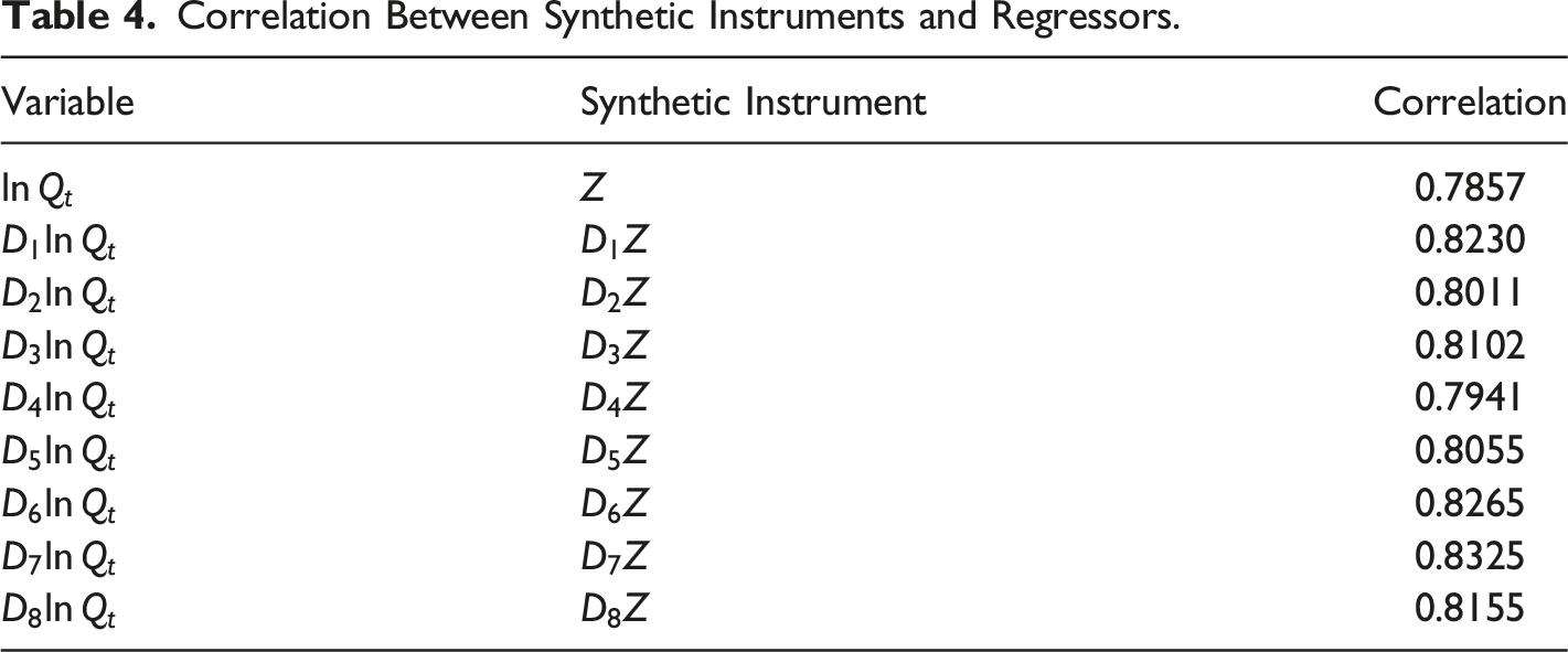
To further restrict the number of instruments, we apply so-called IV instruments for some of the endogenous regressors. Typically IV instruments can be entered into the instrument matrix as a single column per instrument, rather than as multiple columns as occur with GMM instruments, and so are not a cause of instrument proliferation. The problem is finding suitable IV instruments. In one of their models estimated, the seminal paper by Ciccone and Hall (1996) utilizes the presence or absence of a railroad in 1860 as an instrument for a 1988 density index which is an endogenous factor affecting productivity in 1988, on the basis that the early development of railroads underpinned the early development of agglomeration and thus correlates with contemporary density, but is not related to model residuals. Likewise, early patterns of agglomeration and distance from the Eastern seaboard of the USA are additional instruments which correlate with density but are orthogonal to model residuals. While these instruments may be appropriate for their cross-sectional analysis, finding successful time-varying instruments in a panel data context is more demanding. Generally IV instruments that maximize correlation between regressor and instrument tends to also increase the correlation between an instrument and the errors, hence causing the J test to reject, while lesser correlated instruments are typically weak and irrelevant with respect to the endogenous regressors. As explained by Fingleton (2023), and as advocated for cross-sectional regression by LeGallo and Páez (2013), one solution to this dilemma comes from the spatial filtering literature (typically associated with the work of Griffith 1988, 1996, 2000, 2003; Getis and Griffith 2002; Boots and Tiefelsdorf 2000; Patuelli et al. 2006, among others).
Correlation Between Synthetic Instruments and Regressors.
Calculating Direct, Indirect, and Total Effects
The raw elasticities do not fully represent the total effect of a 1 percent change in GDP because spillovers across space contribute to a direct effect, where an increment in GDP in MSA i directly affects productivity in MSA i, an indirect effect where a GDP increment in the other MSAs spills over to affect MSA i′s productivity, with the total effect equal to the sum of the direct and indirect effects. Note that the direct effect will not equal the raw elasticity exactly, because an increment in GDP in i causing a change in productivity in MSA i will cause other MSAs to also increase in productivity, because of the effect of the W ln P
t
term, and these induced productivity changes in neighbours and neighbours of neighbours will spill back to affect productivity in MSA i. The magnitude of these spillover effects can be measured by the difference between the raw elasticities and the direct effects.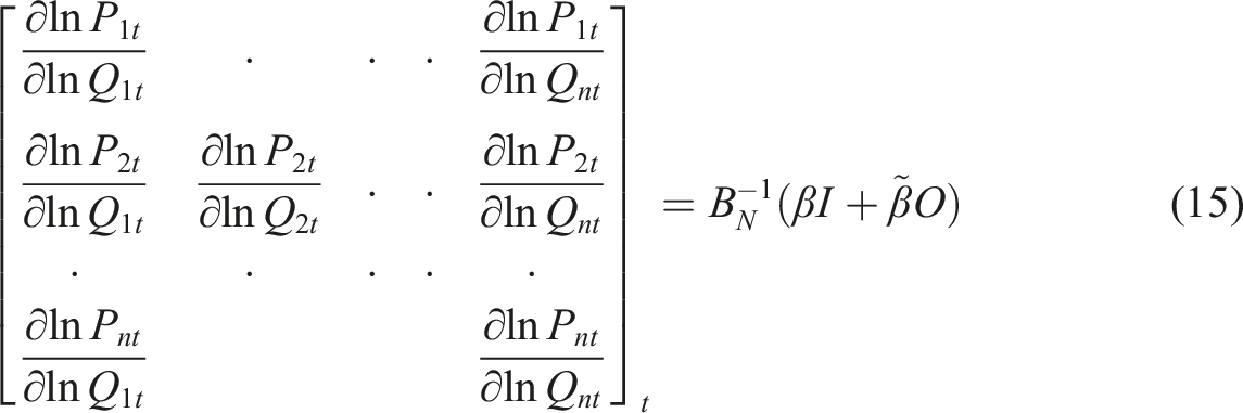
In order to calculate the elasticities that do take these spillovers into account, we calculate the matrix of derivatives (15) in which
Each MSA will have its own elasticity. For example, for i = 1, then we can see from the left hand side of (15) that the first derivative is the elasticity ∂ ln P1t/∂ ln Q1t which is the direct effect of a change in GDP in i = 1 on productivity in i = 1. The other off-diagonal terms in the first row ∂ ln P1t/∂ ln Q
jt
(j = 2, …, n) are the indirect effects. So the total effect of an increment in GDP in all n MSAs on productivity in MSA i = 1 is the row sum of (15). Given the set of MSAs for which parameter estimate
The outcome of applying equation (15) is a set of n direct, indirect and total short-term elasticities, one for each individual. Because each derivative is different, LeSage and Pace (2009) suggest summary measures of direct, indirect and total effects. Accordingly, the direct short-term effect of a unit increase at time t is equal to the mean of the leading diagonal of (15). The total effect is equal to the mean row sum of (15) and the indirect effect is equal to the total effect minus the direct effect. The MSA-specific effects are obtained from the specific rows of matrix (15), so for MSA i, the direct effect is ∂ ln P it /∂ ln Q it and the total effect is the sum of row i. The direct effects tend to be similar to the raw elasticities. The total effects are however very different, since these take full account of the instantaneous spillover effects at time t.
Note that the short-term derivatives in equation (15) pertain to a specific point in time t. If we are prepared to assume constancy of parameters and W over time, and given that the model generating the parameters passes the test of dynamic stability and stationarity, it is also possible to calculate the n by n matrix of long-term derivatives (16), where C
N
= γI + θW, based on effects of a persistent increase in ln Q across all n MSAs as t goes to infinity. So the long-term derivatives are the ones that would hold given that the interactions through space and time have stabilized to a steady-state at which log productivity no longer changes.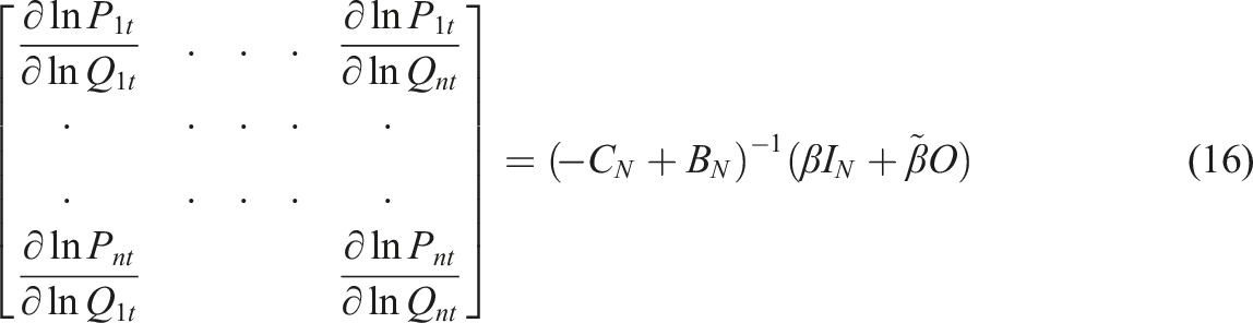
Again the total effect is equal to the mean row sum of (16), and the direct effect is the mean of the main diagonal. And again the elasticities for specific MSAs can be picked out from the matrix of derivatives (16).
The standard errors for each elasticity are obtained by generating numerous (S = 5, 000) sets of parameter combinations based on the estimated k + 4 by k + 4 parameter variance-covariance matrix V for the k + 4 parameters γ, ρ, θ, β, β1…β8. As shown by equation (17), given the decomposition of the estimated parameter variance-covariance matrix via the Cholesky decomposition (chol) to an upper triangular matrix, as described by Elhorst (2014), then the matrix product of this with a k + 4 by 1 vector of samples drawn from an N(0, 1) distribution Φ embodies the covariance, but with zero mean, so adding to this the k + 4 by 1 vector of estimates of [γ ρ θβ β1,…, β8]′ gives outcomes [γ
s
ρ
s
θ
s
β
s
β1s, …, β8s]′ for draw s which has the desired means and covariance.
As noted by LeSage and Pace (2009), the empirical distribution of the parameters can also be obtained using a large number of simulated parameters drawn from a multivariate normal distribution. In this case

Another approach described in LeSage and Pace (2009) obtains dispersion measures base on Bayesian Markov chain Monte Carlo estimation, but this is beyond the scope of this paper. Applying either (17) or (18) gives almost identical outcomes, but the estimates given in Table 8 are based on equation (17).
Each parameter combination drawn (γ
s
, ρ
s
and θ
s
, ; s = 1, …, S) is tested to see if it complies with the dynamic stability and stationarity conditions.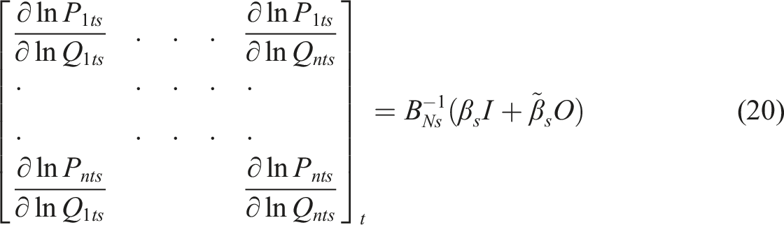
Those that do not are rejected, but the p = 1081 that pass the test are then turned into direct, indirect and total short-term effects using equation (20) in which
Following the approach for short-term derivatives, the distribution of the long-run effects is obtained from the set of P simulations that pass the stationarity test, so from each set of simulated parameters 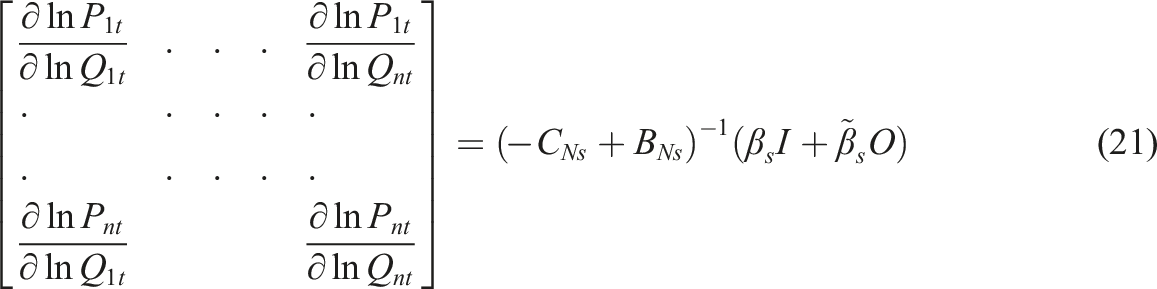
Results
Estimates of Dynamic Spatial Panel Model With Top 8 MSAs.
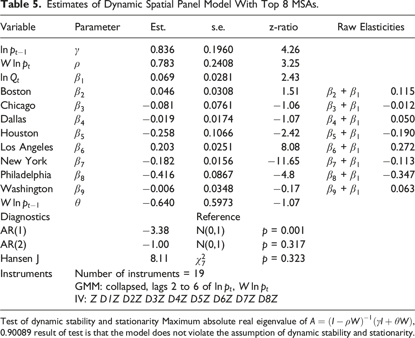
Test of dynamic stability and stationarity Maximum absolute real eigenvalue of
The first critical diagnostic test is of the viability of lagging variable ln P
t
and W ln P
t
by two periods to form GMM instruments, which depends on zero second-order serial correlation in the first differenced residuals (see Arellano and Bond 1991; Bond 2002). An informal indication that this is a reasonable assumption is given by Figure 6 which is based on estimated residuals. Evidence of lack of second order residual serial correlation.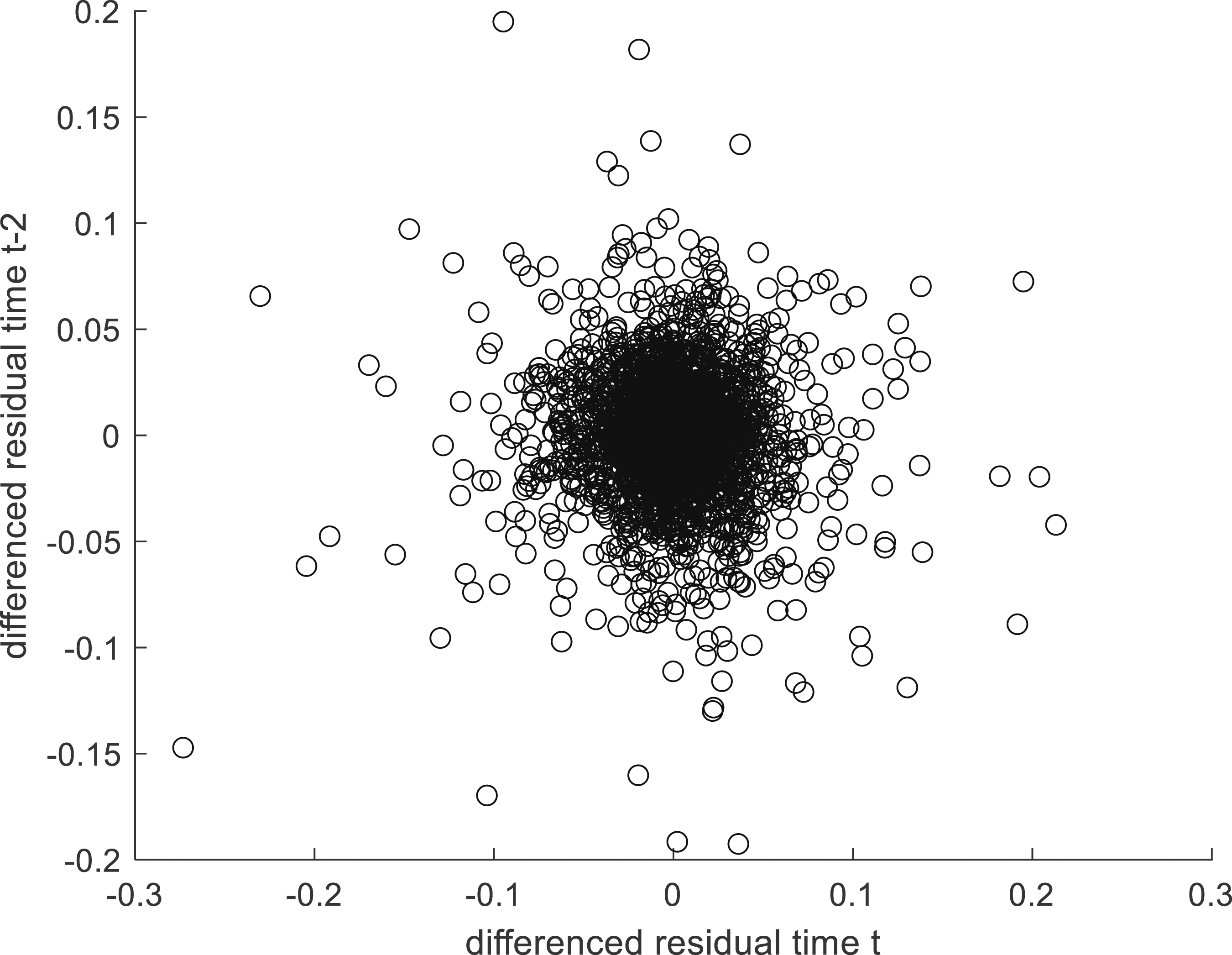
Figure 6 points to an absence of second order serial correlation which is the key requirement. More formally, we reject the null hypothesis of no first-order serial correlation
14
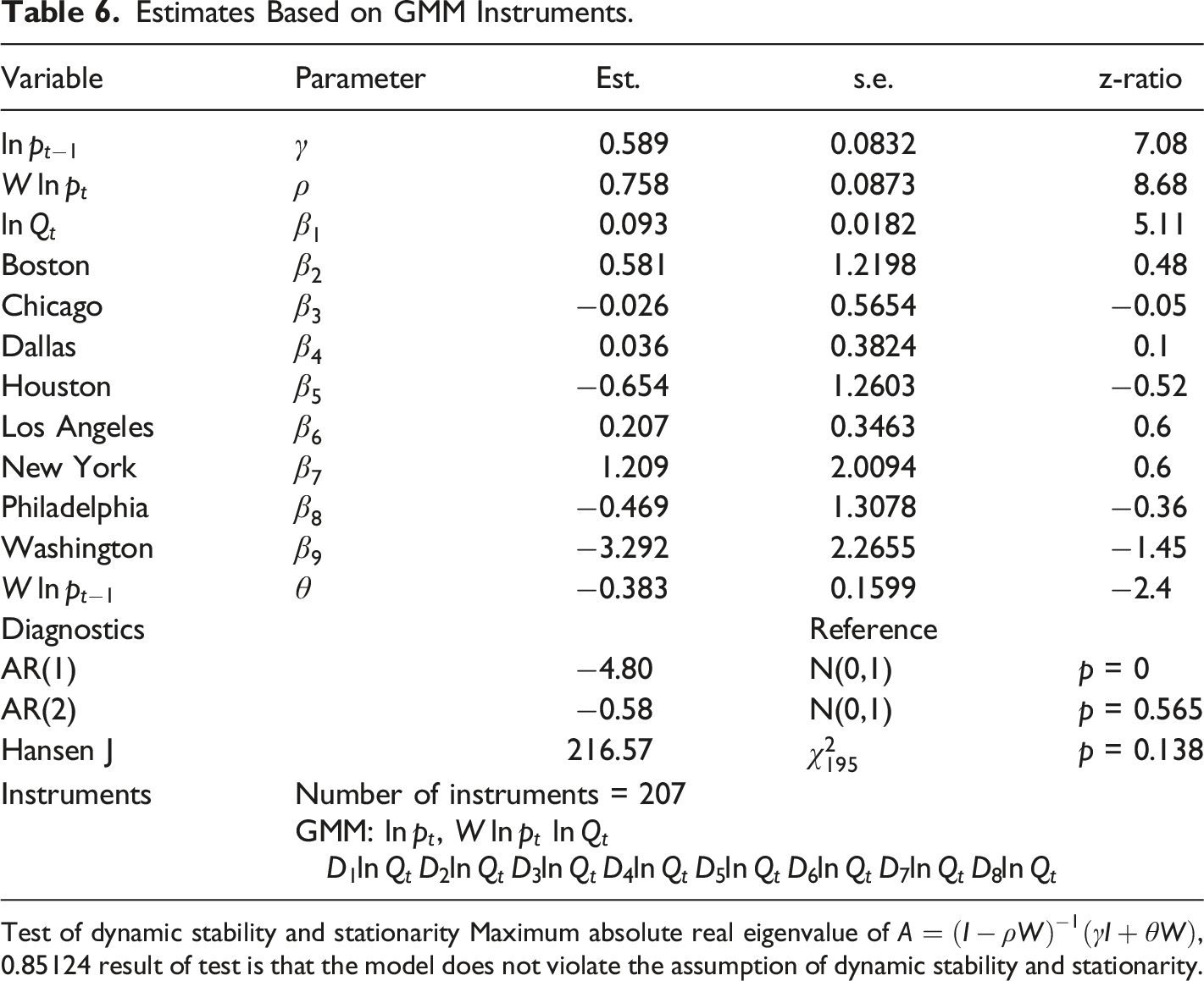
in first differences (AR(1) test) but critically do not reject the null hypothesis of no second-order serial correlation in first differences (AR(2), as shown by Table 5, in which the z-ratio for AR(2) is not extreme with respect to the N(0,1) distribution. So on this basis one can assume that the instruments are independent of the error term which is a necessary requirement for valid instrumental variables. The second crucial diagnostic is the Sargan-Hansen J test for overidentifying restrictions, as described in the Appendix. Typically the J test suffers from low power when there are too many instruments, but this problem has been averted by limiting the use of GMM instruments, collapsing and restricting lags, and applying IV instruments. Table 5 indicates that the estimates are consistent, with the J test statistic not significant when referred to the
The estimates shown in Table 5 indicate that there are highly significant temporal lag and spatial lags, with both
Also we are particularly interested in estimating MSA-specific elasticities, in particular we wish to identify differences in elasticity among the top 8 MSAs and between them and the smaller MSAs. The effect of a 1 percent change in GDP on top 8 productivity has two elements. First it depends, like all other MSAs, on
Estimates Based on GMM Instruments.
Test of dynamic stability and stationarity Maximum absolute real eigenvalue of
Estimates Based on Random Effects GLS.
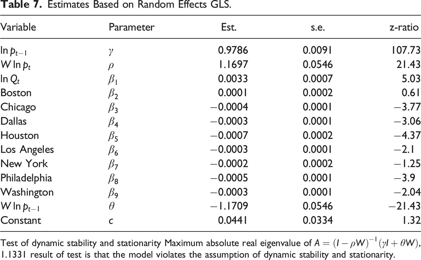
Test of dynamic stability and stationarity Maximum absolute real eigenvalue of
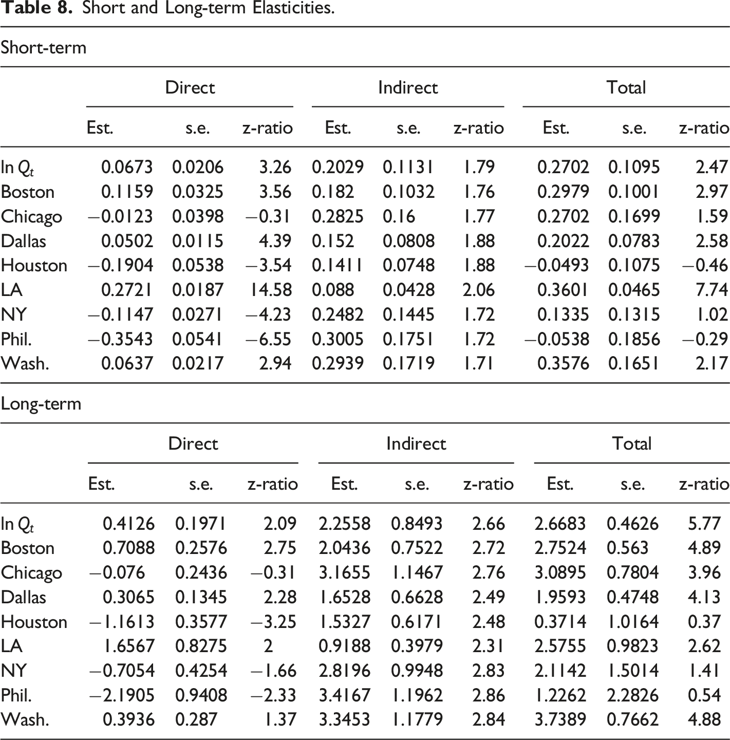
The elasticities in Table 5 are outcomes assuming spillover effects are nullified. However, taking into account spillovers gives the short-term and long-term estimates given in Table 8. Table 8 also gives the standard errors and z-ratios for each of the parameter estimates, using the distribution of the P direct, indirect and total elasticities. In the case of z-ratios greater than 1.96 in absolute value, the 95 percent confidence interval does not include zero, so the parameter estimate is significantly different from zero.
For the smaller MSAs, the estimated short-term total effect of a 1 percent increase in GDP is a 0.27 percent increase in productivity. The outcomes for the top 8 MSAs are varied, ranging from a high total short-run elasticity of 0.36 percent for Los Angeles to −0.05 percent for Philadelphia.
The long-term elasticities in Table 8 are more speculative because they rely on the causes of long-term elasticity to remain constant through time, and are reliant on estimates of parameters made through a period of economic turbulence. A reaffirmation of the stationarity of the estimated model leading to feasible long-run elasticity estimation and a good visual representation of the total long-term elasticities is obtained by iteration. Consider the n by 1 vector 

In equation (23) the n by 1 vector ln Q
T
is the T′th observation of ln Q
t
, t = 1, …, T and D
k
, k = 1, …, 8 is an n by 1 vector of zeros except for 1 in the row specific to top 8 MSA k and β is the k + 1 vector of parameter estimates given in Table 5. Given stationarity,
Repeating the iterations but increasing each variable in X by Δ = 1 gives

Short and Long-term Elasticities.
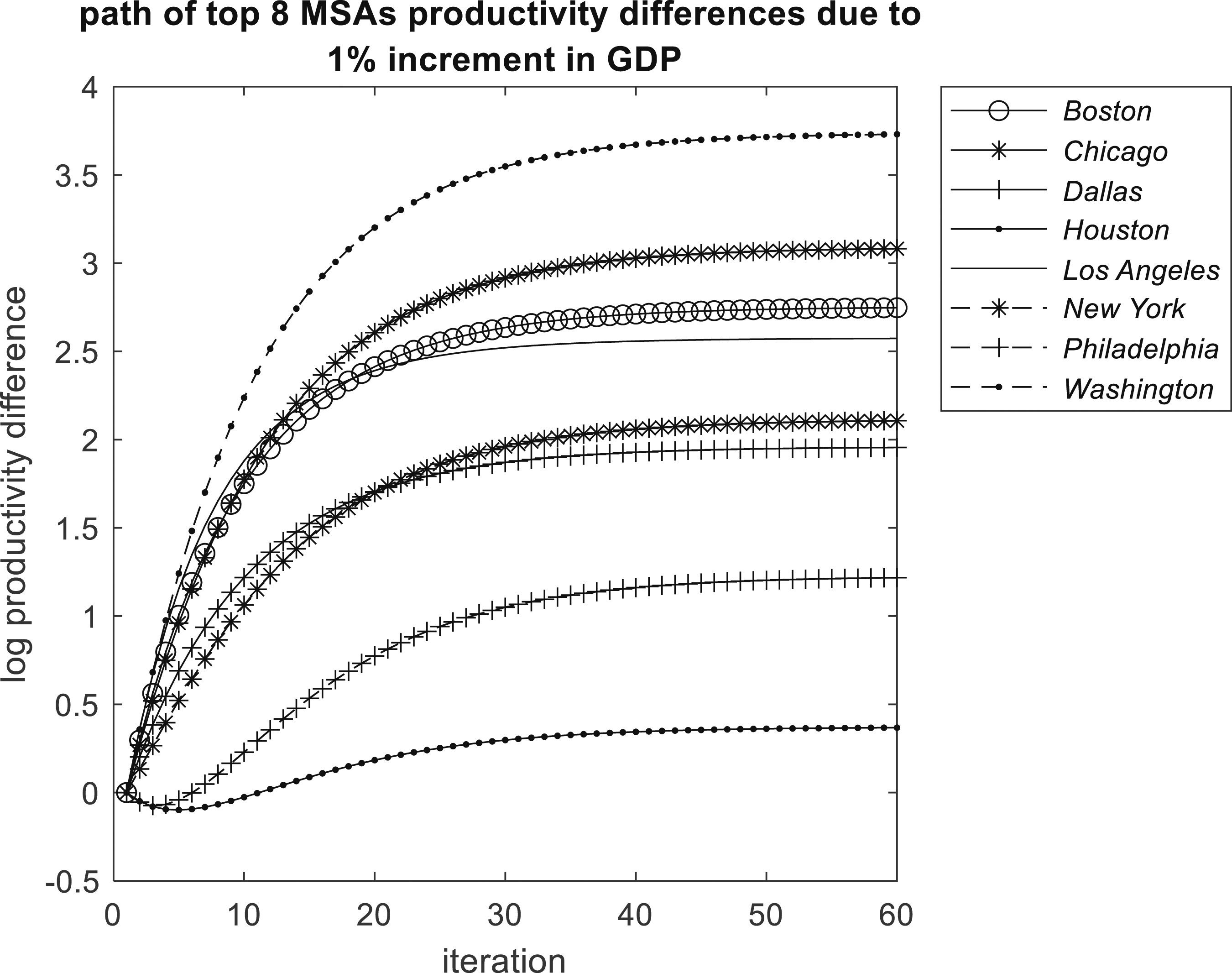
Equilibrium long-run total elasticities.
However it should be emphasized that these results are conditional on parameters estimated over the turbulent period 2011-2021. The negative effects for Houston, for example, undoubtedly reflect the strong negative shocks that Houston experienced through this period, such as the ongoing consequences of the 2008 financial crisis, which had a significant impact on the city’s energy sector, the 2014 oil price crash, which also affected the energy industry, and Hurricane Harvey in 2017 caused significant damage to the city and disrupted many businesses. New York and Philadelphia may have been prone to sector-specific impacts following the financial crisis, and more recently a move to home-based working leading to low office occupancy rates, lost tax revenue and reduced spending on goods and services in central city areas.
Conclusions
This paper shows the significant positive causal effect of GDP growth on productivity growth across the MSAs of the USA, in the context of very limited data at the MSA level, endogeneity and temporal and spatial spillover effects. The paper applies a model driven by theory relating output to productivity, but highlights the diverse nature of this relationship, showing that some of the large MSAs are characterized by output having a significant effect on productivity, but for others the relationship is evidently non-existent. The conclusion is that the broad theoretical link between output and productivity, which is a sine qua non of much of contemporary urban economics and economic geography, is less than law-like when examined at a disaggregated level. The paper shows that Boston, Chicago, Dallas, Los Angeles and Washington stand out as having significant positive total long-run elasticities. This implies that as these agglomerations grow, productivity will advance also, and therefore a range of associated beneficial social and economic attributes, particularly higher wages, should also follow. However the analysis also finds no significant long-run elasticity involving output and productivity for Houston, New York and Philadelphia. This could occur if in the long-run output and labor increased at the same rate leaving productivity constant. Alternatively, while output might increase faster than labor, static or even falling productivity could be due to the inefficiencies of production in a spatially confined urban economy negating the positive externalities one normally associates with large cities, what one might call congestion effects in the broadest sense. One can speculate that this may be the fate of many very large cities, with many producers competing for limited services, property and land, and basically getting in each others way. In the long run, static or falling productivity may dissuade investment. On the other hand the prospect of rising productivity could attract additional investment in physical, social and economic capital. While large cities may not disappear instantaneously, their growth may be stymied because output growth may not induce productivity growth feeding back to further output growth, with static productivity resulting in comparatively low wages and less in-migration. So what we could be observing, if maintained in the long run, is a process of adjustment in city status and an upper limit on city size beyond which negative externalities become dominant. From a policy perspective, this type of outcome could be avoided by encouraging physical and human capital growth and by attempting to minimize negative externalities of congestion by adopting advanced communications technologies and by planning solutions that decentralize congested urban places.
Footnotes
Declaration of Conflicting Interests
The author(s) declared no potential conflicts of interest with respect to the research, authorship, and/or publication of this article.
Funding
The author(s) received no financial support for the research, authorship, and/or publication of this article.