Sage Journals: Discover world-class research

Abstract

Tourism flow is the foundation of tourism development, and studying tourist flows is one of the most important aspects of tourism research. This paper examines tourist flows among A-level scenic spots in Beijing, focusing on local and non-local tourists, utilizing mobile phone data received from Unicom. The research comprises tourist flow distribution characteristics, centrality analysis, community detection, and analysis of affecting factors. The key findings of the study are that tourist distribution is unequal between scenic spots, with non-local tourists having a more concentrated distribution than local tourists. The impact of transport and scenic spot category and level are assessed and tourism links between scenic spots frequented by local tourists and non-local tourists are shown to require different tourism management approaches.

Keywords

Tourist mobility mobile positioning social network analysis community detection

Introduction

World Travel & Tourism Council (2020) reported that the travel and tourism industry is estimated to have contributed 10.3% of global GDP in 2019 and created 330 million job opportunities. Local tourism development has received significant academic attention, with studies in the fields of international tourist flow (Mansfeld, 1990; Shao et al., 2020), tourist behaviors (Loi and Pearce, 2015; Vu et al., 2015), tourist destination loyalty (Tiru et al., 2010), tourist destination identification (Raun et al., 2016), seasonal changes to tourism (Ahas et al., 2007), prediction of tourist movements (Xu et al., 2022), and patterns of tourist attraction systems (Kang et al., 2018; Mou et al., 2020b). Some scholars have emphasized the importance of understanding tourist destinations and movement through time and space (Lew and McKercher, 2006), particularly in the new paradigm of big data, utilizing people’s actual usage and consumption patterns to assist policy implementation on local land use, infrastructure, and transportation planning (Miah et al., 2017). For example, Charles Chancellor (2012) used GPS-track data to extract the flow and patterns of visitor mobility for destination development in North Carolina, in the United States. To explore travelers’ experiences, feelings, interests, and opinions, Marine-Roig and Anton Clavé (2015) and Xiang et al. (2015) retrieved massive volumes of information from travel blogs and online travel reviews. However, for a large geographic region, the mobile phone approach seems to be more desirable for tracking visitors’ mobility in spatial, temporal, compositional, social, and dynamic dimensions at multiscale (Ahas et al., 2007, 2008; Raun et al., 2016; Shoval and Ahas, 2016). Some scholars have recently employed network theory and metrics to further understand the wholeness and complexness of tourist movement and behavior (Liu et al., 2017; Mou et al., 2020a; Xu et al., 2021; Zeng, 2018).

Despite the growing number of studies on inbound tourist flows, little research attention has been given to the differences between flows of local tourists, who work and lives in the city, and non-local tourist, who come and visit from other cities of the country. In general, most tourist attractions do not exist in isolation; they may be fully or partially embedded in local urban systems and linked with urban life, allowing both local and non-local people to benefit from the various advantages of local tourist attractions. The travel purpose and preferences of specific groups of people may, however, be linked to different travel behaviors (Hickman et al., 2015). Numerous previous studies have identified distinct travel behaviors among local and non-local tourists. For instance, these studies have highlighted variations in visitor preferences for nature tourism facilities (Lindberg and Veisten, 2012), disparities in pre-, during, and post-visit outcomes at heritage sites (Gannon et al., 2022), as well as differences in motivation, satisfaction, and loyalty towards cinema events (Báez-Montenegro and Devesa-Fernández, 2017). Thus, it is intuitive that we should differentiate between these two types of individuals (local and non-local) in the local tourism sector. In this vein, this study aims to understand these interactions by evaluating and comparing local and non-local tourism flows in Beijing, the capital of China, in order to improve and enhance tourism management. Beijing is not only a political center but also a city renowned for its rich historical and cultural heritage. It is often referred to as a national garden city and a historical and cultural city. The city boasts 216 Class A scenic spots, which represent a high level of quality in terms of scenic attractions in China. Annually, Beijing attracts over 322 million tourists, both domestic and international (data from 2019). However, being a densely populated global city, Beijing faces challenges related to limited land resources, which in turn affect the availability of supporting facilities for the tourist population. Analyzing the attractions in Beijing can provide valuable insights and lessons for the allocation of attractions and supporting facilities in other global cities. Our study incorporates mobile phone data from Unicom, China, and follows the approach of Ahas et al. (2007, 2008) and Raun et al. (2016), employing several network analysis methods to investigate tourist movements and the key differences across two groups of domestic visitors.

Literature review

Tourism is commonly recognized as a complex system that includes travelers, geographic components such as tourist-generating regions, transit routes, destination regions, and a tourism industry (Leiper, 1979). Understanding tourist destinations and mobility is crucial for transportation planning and tourism management, and it has emerged as one of the profession’s most pressing challenges (Grinberger and Shoval, 2018). Traditional research on tourist destinations and mobility relies mainly on questionnaires, activity diaries, and accommodation records (Leung et al., 2012; Liu et al., 2017; Xing-zhu and Qun, 2014). Recently, it has been observed that big data is causing paradigm shifts since the massive volume of geotagged data from internet and social media can more accurately reflect the respondents’ precise location and time of activity (Girardin et al., 2008; Kitchin, 2014).

According to Li et al. (2018), there are at least three primary types of big data used in tourism research: UGC data (user-generated content), operation data (created by operations), and device data (generated by devices), with current studies focusing primarily on UGC data and device data. Some researchers have specifically used social media data such as Twitter, Flickr, and Instagram to identify tourist spatial-temporal geographic information (Chua et al., 2016; Zhou et al., 2015), to investigate tourist behavior (Vu et al., 2015), and to uncover behavioral distinctions between tourists and locals (García-Palomares et al., 2015; Vu et al., 2015). However, such information is often limited and spatially and temporally skewed (Lo et al., 2011). GPS data, as the most common device data, is frequently used to study tourist behavior (McKercher et al., 2012; Xiao-Ting and Bi-Hu, 2012) and travel suggestions (Zheng et al., 2017). However, GPS data is expensive and time-consuming to gather (Raun et al., 2016), making it less favorable to apply over a large geographic region (East et al., 2017).

In contrast, mobile phone data can cover a broader area and contain more valuable demographic information—for example, where tourists are coming from—than other types of big data (Ahas et al., 2007). A rising number of academics are using mobile phone data to identify tourist locations and assess tourists’ spatiotemporal behaviors, such as tourism’s seasonality (Ahas et al., 2007), destination loyalty (Tiru et al., 2010), repeat visits (Kuusik et al., 2011), tourist flows (Raun et al., 2016). Mobile phone data usability has been successfully tested, and the area of mobile phone data research is rapidly expanding, while also beginning to take into account changes in timescales. Some researchers utilized algorithms to identify 18,000 long-distance excursions taken by 69,000 mobile phone users in France, and examined tourism flows in 32 locations around the country (Vanhoof et al., 2017). To explore changing patterns of tourist flows in scenic spots at different timescales, Qin et al. (2019) used mobile phone bill data to construct a tourist departure–destination matrix of prominent scenic spots in Beijing.

Many scholars have stated that tourist flows between destinations and attractions generate complex, dynamic networks with a variety of opportunities and constraints. Because tourism functions are nonlinear and dynamic, a better understanding of the structure of the complex networks of intourist flows is encouraged (Casanueva et al., 2014). Several researchers examined the destination’s information distribution process using the example of Elba, Italy, and found that cohesiveness and adaptability of stakeholders has a positive impact (Baggio et al., 2010). Complex network analysis provides an important perspective and research tool for tourism flows (Casanueva et al., 2014). To define and measure tourism flows, a variety of network analysis metrics are utilized, including centrality (Zeng, 2018), structural holes (Shih, 2006), network density (Hwang et al., 2006), and clustering coefficients (Mou et al., 2020a). Some researchers used network analysis to investigate attraction networks in Xinjiang and found that regional proximity between the destination’s major attractions is positively correlated with existence of attraction networks, while rank proximity is negatively correlated with attraction networks, implying that attractions of the same rank are primarily competing for tourists (Liu et al., 2017). Distance decay and popularity was shown to affect tourist flows in Qingdao, according to several researchers who integrated classic quantitative and social network analysis (Mou et al., 2020b). Provenzano and Baggio (2019) used the HVG algorithm (horizontal visibility graph) to divide domestic and international tourist networks in Sicily and found that foreign tourist networks were more random and unstable. Others used the community detection algorithm to divide Korean tourist networks into seven groups and investigated differences in destination network structure among tourists from various countries (Xu et al., 2021).

Given that the local tourism market is not homogenous (McKercher et al., 2012; Xu et al., 2021), several studies endeavored to further explore the spatiotemporal behaviors of different sub-groups of tourists in tourist destinations, including different nationalities of origin (Xu et al., 2021); single-day and multi-day tourists (Rodríguez et al., 2018); first-time and repeat tourists (McKercher et al., 2012); and different tourist group sizes (Zhao et al., 2018). Xu et al. (2021) employed a community detection algorithm to study several tourism regions and found that tourists from different countries tended to have distinct regional preferences in South Korea—the most popular attractions for visitors from Asian and Western countries were to Jung-gu, whereas visitors from the Philippines mainly sought the islands and coastal areas.

To our knowledge, there is still a scarcity of evidence on the differences between local and non-local tourist flows through the lens of complex networks, especially in global cities. Even among attractions of the same level, there can be significant variations in visitor profiles, including differences in motivations, behavior preferences, and satisfaction levels. By segmenting the population, researchers studying urban areas can more effectively identify distinct travel patterns among different groups of tourists. Thus, this study further subdivides domestic tourists into two groups and offers insight into whether the local and non-local tourists’ movements and behaviors correspond show distinct destination preferences. To achieve this, the study uses large-scale monthly mobile phone data to measure the network of connections formed between attractions, and aims to explore the differences in tourism destination and interactions between local and non-local tourists. This approach compensates for the limitations of small-sample data often collected through questionnaires or travel diaries in previous studies. Furthermore, novel methods such as community detection are applied to explain the characteristics of attractions and their connections to multiple tourist groups at the city level. This fills existing gaps in data methodology and provides a more comprehensive understanding of the subject matter.

Study area and mobile phone dataset

In general, China used its own rating system for tourist attractions, based on uniqueness and recognition of the sightseeing offering; tourist attractions were graded on a scale from A to AAAAA. For example, Forbidden City and Summer Palace in Beijing are 5A attractions. The newest list of A-level attractions was published on the official website of the Beijing Municipal Culture and Tourism Bureau as of October 2019 and features 223 entries. This study used Baidu Map’s AOI (Area of Interest) data to define these tourist attraction boundaries and identified 216 A-level scenic locations in total, including nine 5A scenic spots, 72 4A scenic spots, 106 3A scenic spots, and 28 2A scenic spots, accounting for 96.9% of all scenic spots (Figure 1).

Figure 1.

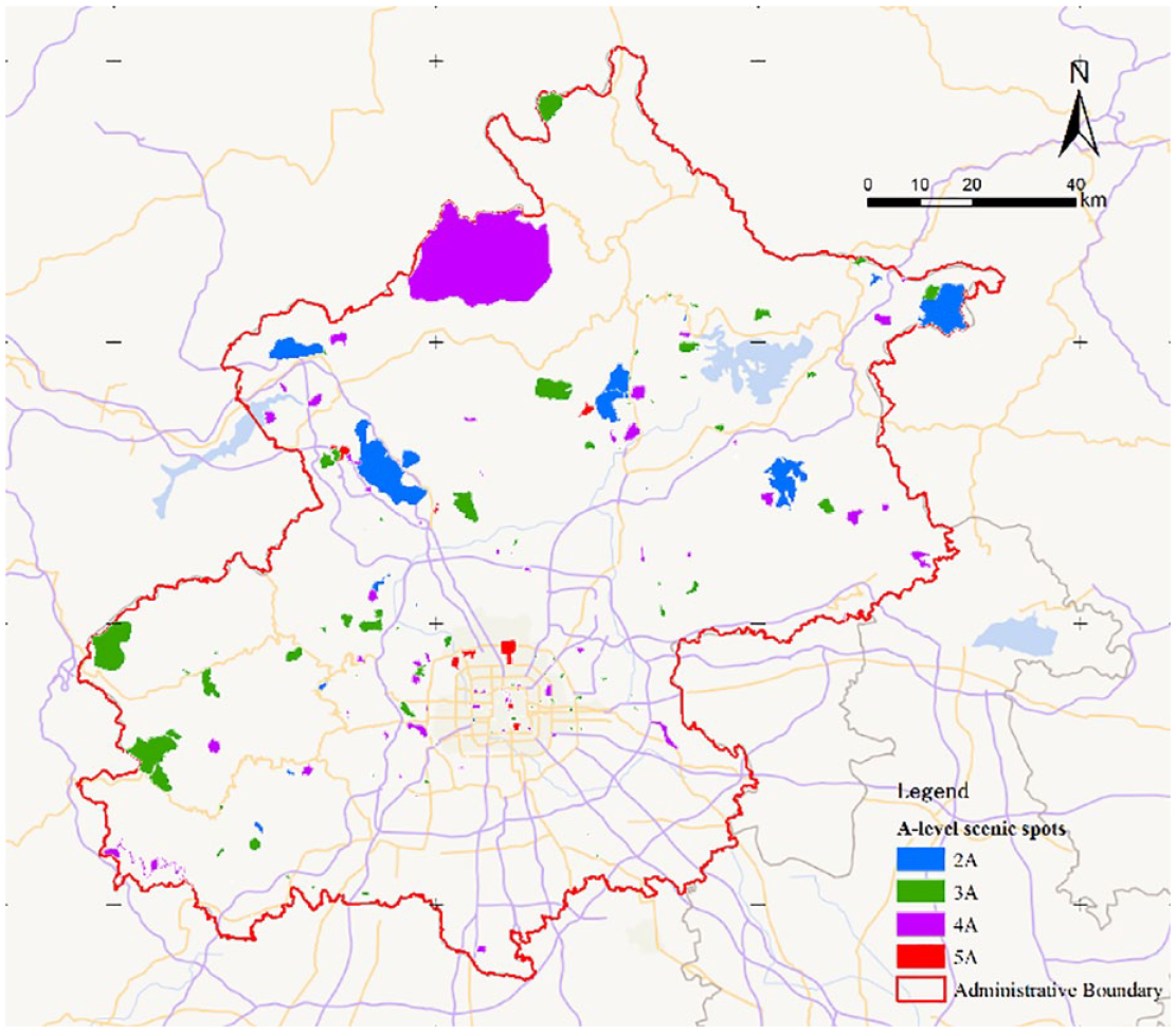
Distribution of 216 A-level scenic spots in Beijing.

Our mobile phone data came from China Unicom, one of China’s three major mobile operators, which, according to government figures, had 31.55% of users in Beijing in 2019. Table 1 provides the records of individual mobile phone data users, including the user’s unique mobile phone ID, place of residence ID card, date, and whether the user is a local traveler or not. It is noted that China Unicom identified people as local residents if they work and live in a place for more than 15 days within any month, with the rest of the people labeled as non-local people. Based on this, we further defined tourists as people that spent more than 0.5 hours in tourist attractions based on the records from the mobile phone base station.

Table 1.

Example of an individual’s mobile phone records in the dataset.

User ID	Id area	Date	Starting Time	Ending Time	Longitude	Latitude	Is local
922***	V0410100	20201101	8:50	9:53	116. ***	39. ***	N
922***	V0110000	20201101	13:59	14:26	116. ***	40. ***	Y
922***	V0220500	20201101	15:07	16:43	116. ***	40. ***	N
. . .	. . .	. . .	. . .	. . .	. . .	. . .	. . .
922***	V0110000	20201101	17:33	19:46	117. ***	40. ***	Y
922***	V0110000	20201101	22:27	22:56	117. ***	40. ***	Y

***

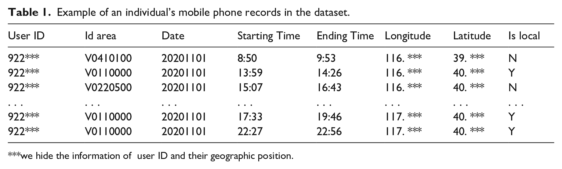
we hide the information of user ID and their geographic position.

Descriptive statistics of tourists

Our dataset determined the tourist population in 216 A-level scenic locations in Beijing in November 2020. The overall tourist population of 214 scenic locations was 5,534,600 in November 2020, with an average daily total tourist population of 184,500, consisting of 4,475,700 local tourists and 1,058,900 non-local tourists. Figure 2 depicts the tourist volume distribution of 214 scenic spots. Due to their tiny size and remote location, two scenic spots were not classified as tourist destinations. Every scenic spot identified local tourists, while four scenic spots did not identify non-local tourists.

Figure 2.

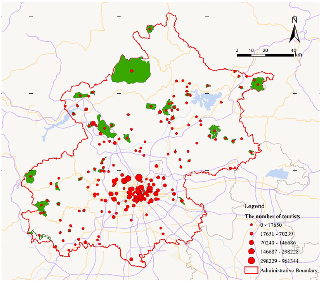
The number of tourists to 214 A-level scenic spots in Beijing.

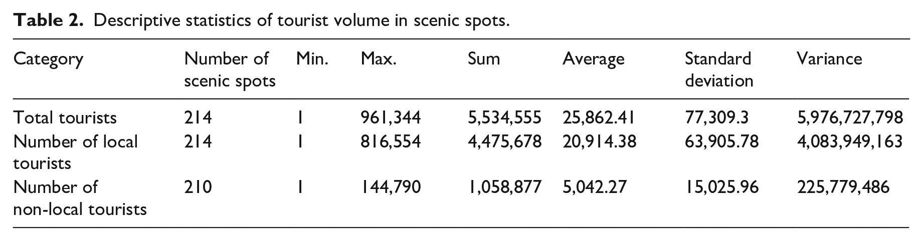
Table 2 shows descriptive statistics on the number of tourists visiting each scenic spot, as well as the number of local and non-local tourists. The average number of tourists per scenic spot was 25,862, comprising 20,914 local tourists and 5,042 non-local tourists. Beijing Olympic Park, which also had the highest number of local and non-local tourists, had the highest number of tourists in November among all A-level scenic locations, with 961,300 tourists. According to research, Beijing Olympic Park is located in the northern end of the Beijing city axis, and it is also the only 5A scenic spot that does not charge admission fees; it is a comprehensive regional public activity center for citizens and has two subway lines passing through it.

Table 2.

Descriptive statistics of tourist volume in scenic spots.

Category	Number of scenic spots	Min.	Max.	Sum	Average	Standard deviation	Variance
Total tourists	214	1	961,344	5,534,555	25,862.41	77,309.3	5,976,727,798
Number of local tourists	214	1	816,554	4,475,678	20,914.38	63,905.78	4,083,949,163
Number of non-local tourists	210	1	144,790	1,058,877	5,042.27	15,025.96	225,779,486

Centrality metrics in network analysis

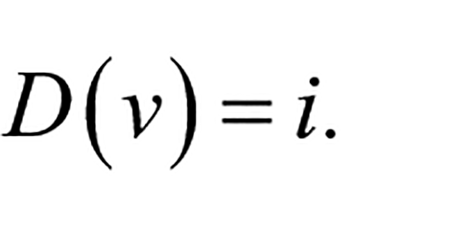
There are at least three common centrality metrics in network analysis, including degree, closeness, and betweenness. The degree of a vertex is its most basic structural property, defined as the number of its adjacent edges. Degree centrality reflects the degree to which a node in the network is directly related to other nodes. If there are N nodes in the network, and node v is directly connected to i nodes with edges, then the degree of the node is:

D (v) = i .

Closeness centrality measures how many steps are required to access every other vertex from a given vertex (Freeman, 1978). The closeness centrality of a vertex is defined by the inverse of the average length of the shortest paths from all the other vertices in the network. The closeness centrality of node v in an unweighted network is defined as:

C (v) = \frac{1}{\sum_{i \neq v} d_{v} i}

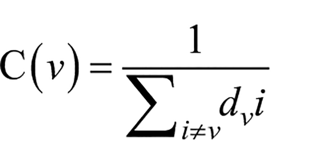
where d_v is the shortest path from node v to the other vertex (node |i).

The notion of betweenness is defined by the number of geodesics (shortest paths) going through a vertex or an edge (Brandes, 2001). Betweenness reflects the role and influence of a certain node in the network. When calculating all the shortest paths between any two nodes in a certain network, a higher betweenness centrality of a node indicates that there are more shortest paths passing through that node. The betweenness centrality of node v in an unweighted network is defined as:

B (v) = \sum_{i \neq j, i \neq v, j \neq v} g_{i v j} / g_{i j}

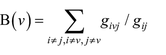
where g_ij is the number of paths from node i to node j, g_ivj is the number of paths by node v in the paths from node i to node j.

Community detection in network analysis

The community detection algorithm developed rapidly in network theory, and could help to understand the degree to which a node interacts with neighboring nodes in the network (Clauset et al., 2004). Nodes within the same community are tightly connected to each other, while connections between communities are sparser. The multilevel algorithm is considered to be one of the better community detection algorithms in terms of accuracy and computation time (Javed et al., 2018; Yang et al., 2016). It is based on the modularity measure and has a hierarchical approach. Initially, each vertex is assigned to a community on its own. In every step, vertices are reassigned to communities in an greedy way: each vertex is moved to the community with which it achieves the highest contribution to modularity. When no vertices can be reassigned, each community is considered a vertex on its own, and the process starts again with the merged communities. The process stops when there is only a single vertex left or when the modularity cannot be increased any more.

Modularity calculates the modularity of a graph with respect to the given membership vector (Clauset et al., 2004). The modularity of a graph with respect to some division (or vertex types) measures how good the division is, or how separated are the different vertex types from each other. It is defined as:

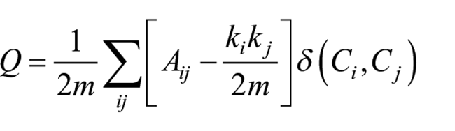
Q = \frac{1}{2 m} \sum_{i j} [A_{i j} - \frac{k_{i} k_{j}}{2 m}] δ (C_{i}, C_{j})

where m is the number of edges, A_ij is the element of the A adjacency matrix in row i and column j, k_i is the degree of i, k_j is the degree of j, C_i is the type of i, C_j that of j, the sum goes over all i and j pairs of nodes, and $δ (x, y)$ is 1 if x = y and 0 otherwise.

Empirical analysis

Regional inequality of tourists

We employed the Gini coefficient to measure the inequality of travel flow between scenic spots in Beijing. The Gini coefficient is 0.803, with the top 54 of the 214 scenic spots having 87.6% of the tourists, indicating that the disparity of tourists among scenic spots is very large, implying that the majority of scenic spot tourists are concentrated in a small number of A-level scenic spots, which is consistent with the distribution pattern of visitor destinations observed in previous studies (Mou et al., 2020a; Xu et al., 2021).

When we further sub-divide the travelers, the Gini coefficient for local residents is 0.781, whereas the Gini coefficient for non-local tourists is 0.888 (Figure 3). This finding suggests that both local and non-local visitors visit a small number of core A-level scenic places during their trips, with non-local travelers being more focused on scenic spots than local tourists. Considering the geographically dispersion of Beijing’s scenic spots, the distribution of non-local tourists tend to be more diverse, as that non-local tourists may have a higher level of travel purpose.

Figure 3.

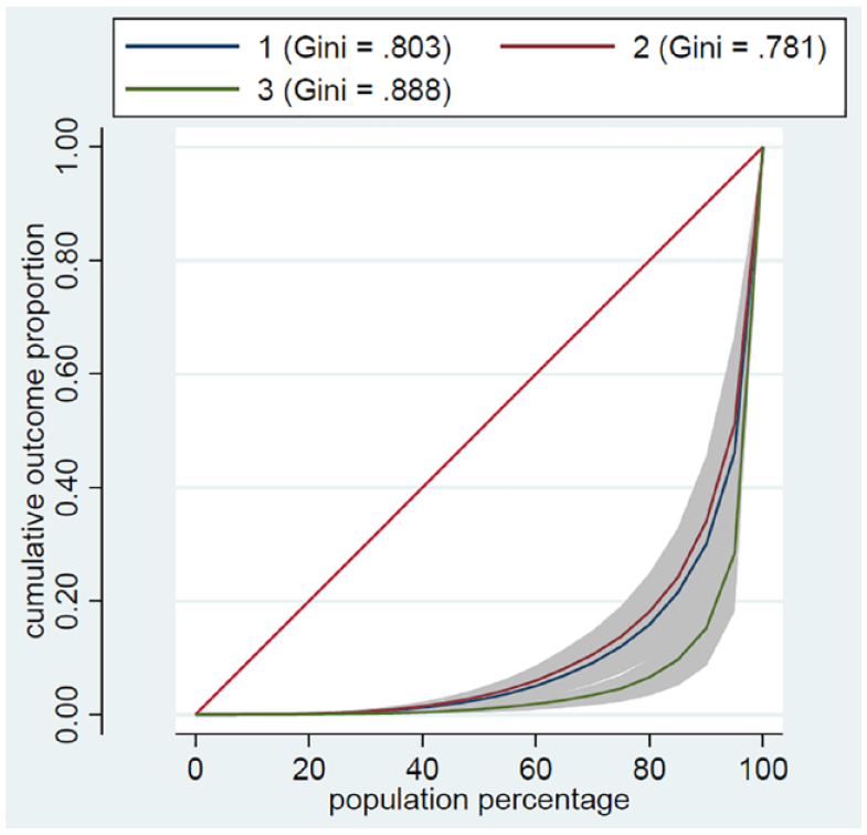
Gini coefficient of tourists (1 for total tourists, 2 for local tourists, 3 for non-local tourists).

Pattern and centrality analysis of the tourism flow network

Our mobile data revealed a total of 3,428 pairs of travel links between 200 scenic spots, resulting in 79,600 tourist trips. A total of 3,101 pairs of local visitors’ scenic travel connections were found, involving 200 scenic spots and 46,600 trips. The total number of scenic area travel contacts for non-local residents is 1,717 pairs, with 33,000 journeys involving 165 scenic spots. Figure 4 shows that the A-level scenic spots in central Beijing are closely linked to one another, forming a polycentric network pattern. Some of the Badaling Great Wall in the northwest is also clearly integrated into the network structure, becoming one of the network’s poles. Beijing’s outer scenic spots are less connected to one another and more reliant on the city’s other major scenic spots. The peripheral centers also include Beijing Safari Park in the south, Shidu Scenic Area in the southwest, and some scenic spots in the northeast such as Yanqi Lake Scenic Area and Mutianyu Great Wall. The network density for the entire network is 0.17, which shows the ratio of scenic sites to connections between scenic spots.

Figure 4.

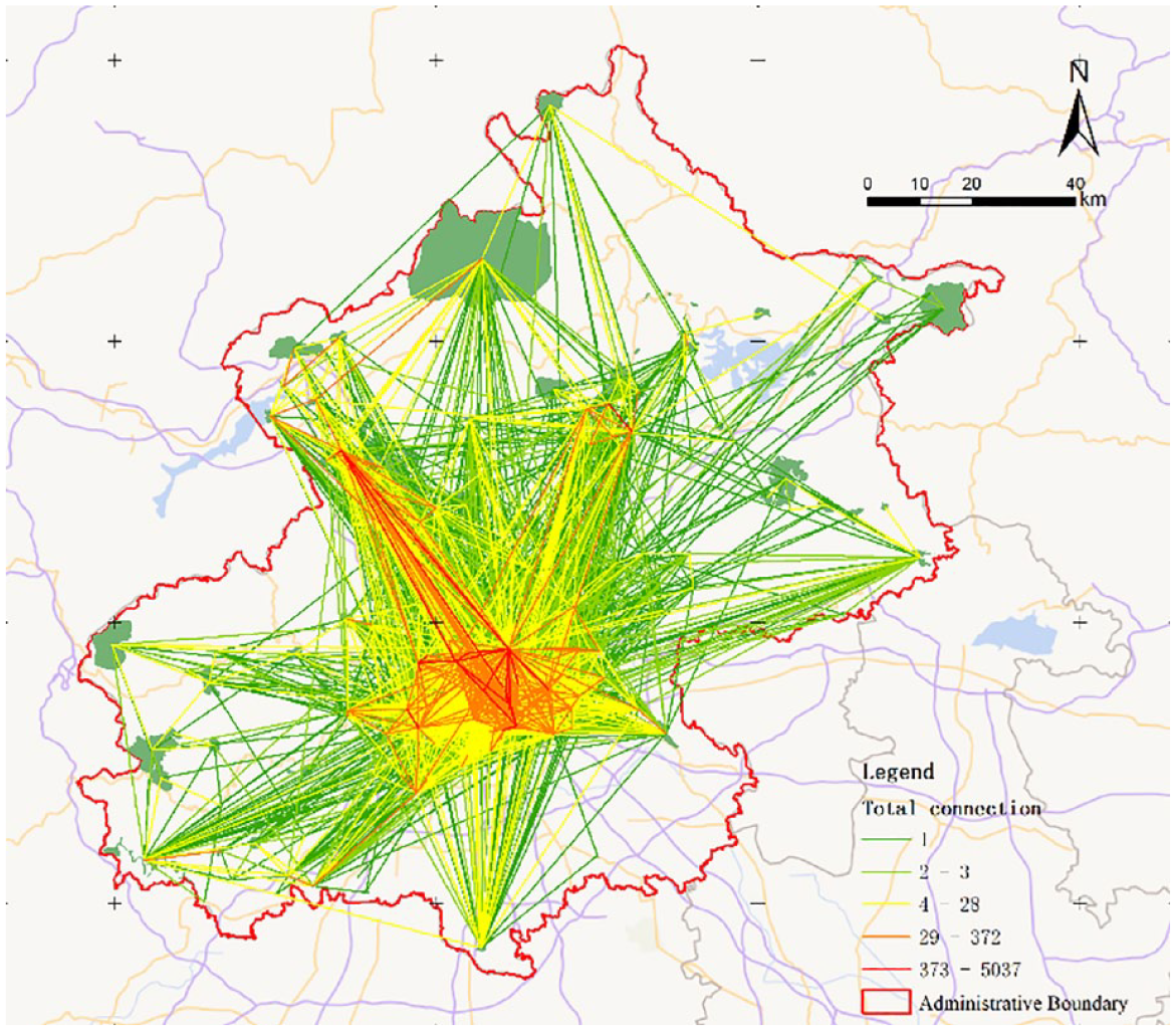
Tourism links between 200 scenic spots.

Figure 5 shows the travel patterns of local tourists (a) and non-local tourists (b). It is seen that the network intensity and network coverage area of local tourists are significantly higher than those of non-local tourists, with non-local tourists having a network density of 0.16, compared to 0.13 for local tourists. However, the network structure of both is similar—polycentric—with an area of high connections located in the central urban area and the Badaling Great Wall attraction. It may confirm the most popular attractions and route choices on parade for local and out-of-town tourists for some consistency in Beijing, and local residents’ travel preferences are more diverse and leisurely.

Figure 5.

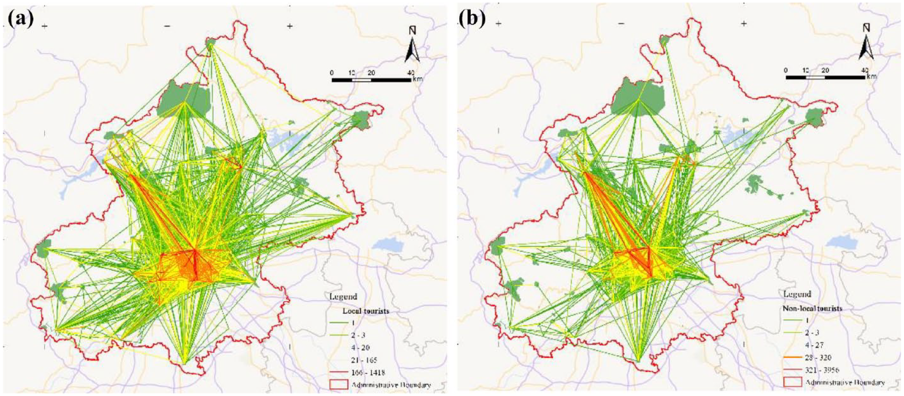
Tourist links between scenic spots: local tourists (a) and non-local tourists (b).

The degree centrality of a scenic area represents the scenic area’s aggregation and radiation capacity, showing the tourist linkage of scenic spots with other scenic spots within the tourism flow network. Scenic spots having a high degree of centrality can be regarded as the network’s key tourist attractions. Figure 6 shows the degree centrality of 206 scenic locations. When it comes to the distribution of scenic spot centrality, the highest values are concentrated in the central city, while the lower values are dispersed throughout weaker areas, such as the suburbs on the edges of Beijing. Tourists prefer northern attractions over those in the southwest when it comes to the centrality of attractions. For the degree centrality of total and local visitors, Olympic Park, Chaoyang Park, Yuanmingyuan Park, Qianmen Avenue, and Beijing Garden Expo Park are in the top five, while for the degree centrality of non-local visitors, Forbidden City and Summer Palace replaced Beijing Garden Expo Park and Qianmen Avenue in the top five.

Figure 6.

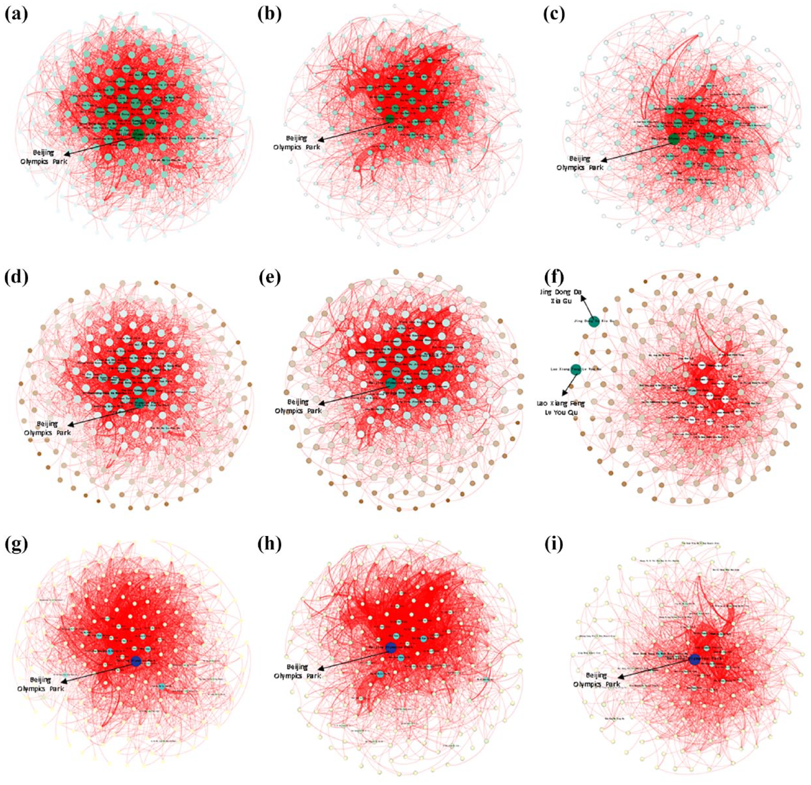
Degree, closeness centrality, and betweenness centrality of scenic spots. (a) Total degree. (b) Degree of non-local. (c) Degree of local. (d) Total closeness. (e) Closeness of non-local. (f) Closeness of local. (g) Total betweenness. (h) Betweenness of non-local. (i) Betweenness of local.

The scenic spots with the highest closeness centrality are primarily found in the core and northern peripheral areas, while those with the lowest are primarily found in the southwestern periphery areas. The Beijing Olympic Park has the greatest closeness centrality. Local tourists choose the northern scenic places, such as Qianmen Avenue, while non-local tourists prefer the Badaling scenic spot clusters, according to the closeness centrality of local and non-local travelers. In contrast, the stronger the irreplaceability of a spot for the flow of tourists between attractions and the larger the flow via the spot, the higher the betweenness centrality. Because tourism access is blocked if a scenic place is withdrawn from the tourism flow network, certain scenic spots will see a decrease in tourists. The Beijing Olympic Park has the highest betweenness centrality of all. When comparing the betweenness centrality of local and non-local visitors, it is clear that the high values for non-local tourists are more spread. With the exception of scenic spots in the middle area, local tourists’ high betweenness centrality is primarily spread in the north, whereas non-local tourists’ high betweenness centrality is primarily dispersed in the southeast.

The associations of travel flow and attraction features

Multiple elements such as tourist conditions, destination characteristics, transportation characteristics, macro environment, and unforeseen circumstances have been demonstrated to influence tourism flows (Lew and McKercher, 2006; Zeng and He, 2018). The goal of this study is to learn more about the factors that influence tourism flow. The independent variables are two categories of scenic characteristics and transportation conditions: the former includes scenic category, scenic area, scenic rating, ticket price, and opening hours, and the latter includes the number of subway stations within 500 and 1,000 meters.

Diverse scenic spots in the Beijing tourism network may be grouped into three categories: urban leisure, historical and cultural, and natural landscape, combined with the primary types of resources on which each tourist attraction is built. There are 104 urban leisure-type scenic locations, 56 historical and cultural-type scenic spots, and 56 natural scenic spots among the 216 scenic spots primarily investigated. The number of subway stations within 500 meters and 1,000 meters spatial distance of each scenic spot can be counted for accessibility and traffic conditions. The rank and ticket price of scenic areas may be found on the Beijing tourism website, which combines the ticket price and opening hours of scenic spots with data from services like Meituan, Dianping, and Ctrip for verification and supplementation.

The tourism flow characteristics are divided into five categories: tourist volume (T), linkage (L), degree centrality (DC), closeness centrality (CC), and betweenness centrality (BC) of the scenic spot, each of which includes the total number of tourists in the scenic area (T), local tourist characteristics (A), and non-local tourist characteristics (E), yielding 15 variables. The tourist volume here is defined as the total number of tourists who visited a specific scenic spot, while linkage is defined as the number of tourists who departed from one scenic spot to visit other spots. Using a linear regression model, these 15 tourism flow characteristics are recognized as dependent variables and the scenic area-related variables as independent variables (Table 3). The two independent variables utilized as reference factors were urban leisure-type scenic spots and 3A-class scenic spots.

Table 3.

Regression analysis results.

Variable	TT	AT	ET	TL	AL	EL	TDC	ADC	EDC	TCC	ACC	ECC	TBC	ABC	EBC
Ticket prices	−0.295	−0.315	−0.146	−0.819	−1.000	−0.146	−0.051	−0.096	−0.460	−0.194	−0.058	−0.699	−0.297	−0.593	−0.789
Opening hours	0.676	0.641	0.739	0.841	1.097	0.739	6.301***	6.368***	4.011***	2.948**	3.702***	1.472	1.891	2.434*	1.432
Historical	−2.717**	−2.795**	−1.875	−1.560	−2.382*	−1.875	−2.007*	−2.200*	−0.916	−1.579	−1.452	−0.669	−1.130	−0.897	−0.434
Natural	−0.811	−0.811	−0.678	−0.653	−1.053	−0.678	−4.839***	−4.641***	−3.452**	−5.316***	−5.144***	−4.682***	−0.144	−1.107	−1.005
2A	−0.082	−0.092	−0.021	−0.010	0.007	−0.021	−1.311	−1.398	−0.372	−0.575	−1.070	−1.011	−0.574	−0.766	−1.381
4A	0.862	0.813	0.961	1.541	2.028*	0.961	4.469***	4.230***	3.784***	3.403**	3.473**	−0.045	2.858**	3.141**	1.768
5A	8.120***	6.937***	12.677***	11.982***	8.827***	12.677***	6.740***	6.268***	8.800***	2.304*	2.550*	1.013	3.309**	2.734**	5.352***
Area	0.716	0.718	0.590	0.273	0.315	0.590	2.136*	2.047*	1.348	2.447*	2.160*	1.314	1.644	1.741	1.625
500 m subway stations	7.974***	7.855***	7.235***	6.718***	7.409***	7.235***	7.345***	7.561***	8.377***	0.955	0.830	1.677	1.938	0.799	3.487**
Constant	−0.134	−0.093	−0.317	−0.246	−0.181	−0.317	−1.795	−1.944	−1.093	14.605***	14.243***	14.390***	−0.072	−0.332	0.085
adjusted R-squares	0.498	0.461	0.603	0.591	0.528	0.574	0.633	0.631	0.666	0.270	0.294	0.201	0.149	0.132	0.309
sig.	0.00	0.00	0.00	0.00	0.00	0.00	0.00	0.00	0.00	0.00	0.00	0.00	0.00	0.00	0.00
	Total number of tourists	Number of local tourists	Number of non-local tourists	Total linkage of tourists	Local tourist linkage	Non-local tourist linkage	Total degree centrality	Local tourist degree centrality	Non-local tourist degree centrality	Total closeness centrality	Local Tourist closeness centrality	Non-local Tourist closeness centrality	Total betweenness centrality	Local tourist betweenness centrality	Non-local tourist betweenness centrality

Variable	TL	TAC	TEC	ITC	ITAC	ITEC	OTC	OTAC	OTEC	CTAC
Distance	−6.376***	−7.952***	−2.932**	−6.301***	−7.706***	−3.495***	−2.750**	−2.884**	−2.038*	−2.098*
Constant	10.991***	13.530***	6.501***	9.655***	11.925***	5.801***	4.122***	4.494***	3.141**	4.889***
adjusted R-squares	0.011	0.020	0.004	0.019	0.031	0.010	0.016	0.019	0.017	0.004
sig.	0.00	0.00	0.00	0.00	0.00	0.00	0.01	0.00	0.04	0.00
	Tourist linkage	Local tourist linkage	Non-local tourist linkage	Tourist linkage inside	Local tourist linkage inside	Non-local tourist linkage inside	Tourist linkage inside	Local tourist linkage inside	Non-local tourist linkage inside	Local tourist linkage cross

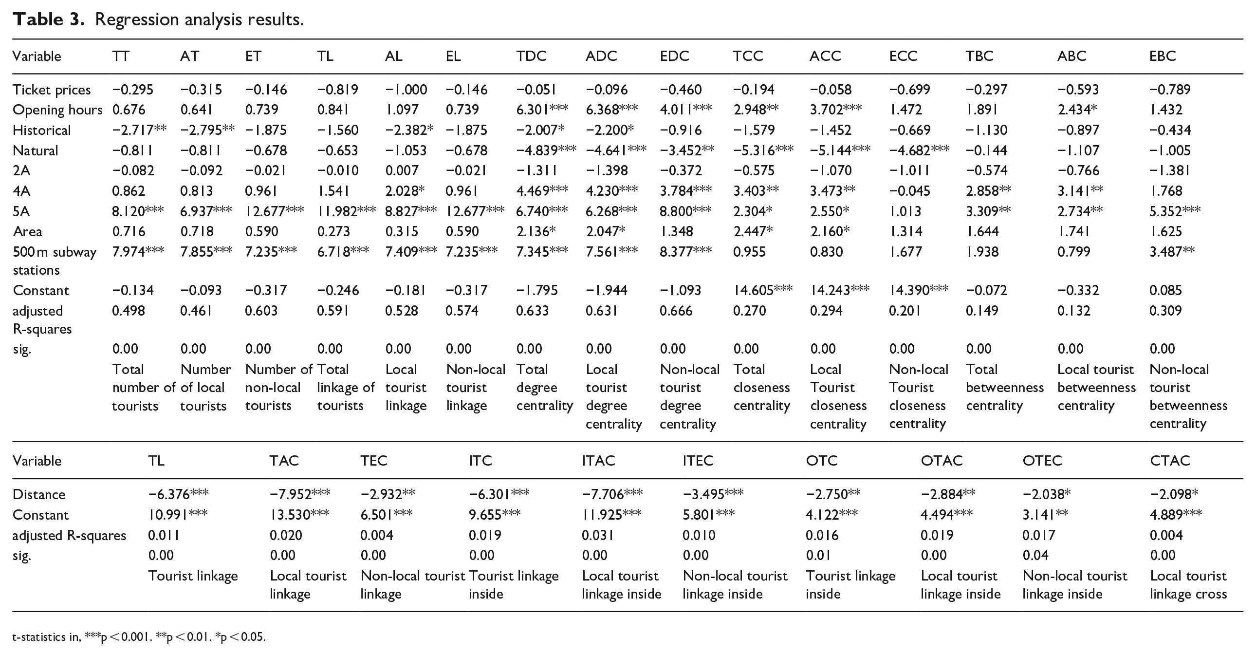
t-statistics in, ***p < 0.001. **p < 0.01. *p < 0.05.

Seven independent variables were significant in terms of their dimensions: scenic spot opening hours, historical and cultural-type scenic locations, natural scenic spots, 4A-class scenic spots, 5A-class scenic spots, scenic spot area, and the number of subway stations within 500 meters. Two factors, ticket price and 2A-class scenic spot, were not significant in all models, indicating that tourists may not consider low-class scenic spots or ticket price while picking a scenic spot. We found that 70 (32.7%) of the 214 picturesque spots studied were free. When compared to higher-priced scenic sites, free and low-cost scenic spots offer similar tourism resources.

In all 14 models (Table 3), 5A-class scenic spots are significant, with the exception of the model of non-local tourists’ closeness centrality (ECC), showing that non-local visitors are less likely to be influenced by this factor while traveling between scenic spots. Furthermore, when compared to 5A-class scenic spots, 4A-class scenic spots have a greater impact on scenic spot centrality aspects such as all types of degree centrality, closeness centrality, and betweenness centrality of total and local visitors, while having no impact on all types of tourist volume and linkage. This could indicate that only 5A-class scenic places have a major impact on tourists’ scenic destination choices, while 4A-class scenic spots have little impact. The number of 500 meter subway stations comes next, which is significant in 10 models but only insignificant in the models of total and local tourists’ closeness centrality and betweenness centrality (TCC, ACC, ECC, TBC, ABC).

For the category of scenic spots, historical- and cultural-type scenic spots were significant in five models: total tourists, total degree centrality of scenic spots, local tourist volume of scenic spots, local tourist connectedness, and degree centrality of local tourists. The natural landscape scenic area, on the other hand, exhibits a more opposing trait, which has no bearing on the number of visitors or connectedness of the scenic area, but does have an impact on its degree of centrality and closeness centrality. These models demonstrate detrimental implications for both historical and cultural scenic locations as well as natural scenic spots. Most tourists prefer urban leisure-type scenic locations to these two categories of scenic spots, which could be the explanation behind this.

We discovered that the opening hours of scenic spots were significant in five models, including all sorts of scenic spot degree centrality, as well as total tourists and local tourists’ closeness centrality. 185 beautiful spots (86.4%) were available for at least eight hours, according to data analysis. Local tourists may generally reach from one scenic spot to another within this distance, however non-local tourists may not be affected because of the closeness centrality of scenic spots.

In terms of dependent variables, we find that the number of historical and cultural scenic spots, 5A-class scenic spots, and 500 meter subway stations have an impact on tourist volume and linkage. However, historical and cultural scenic spots have a negative impact on local tourists, while there is no significant impact on non-local tourists. This suggests that local tourists are less inclined than non-local tourists to consider historical and cultural scenic sites when they are choosing scenic spots to visit.

For all nine models involving centrality, we found that scenic degree centrality was the most important, followed by closeness centrality, with the least significant being betweenness centrality, 4A scenic areas, 5A scenic areas, and the number of 500 meter subway stations. This means that if we want to improve the distance between some scenic spots on tourist routes, we need to renovate the scenic spots and improve traffic conditions in tourism management.

Scenic connection network and distance decay effect

Furthermore, the study hopes to further investigate whether the linkage between scenic areas is influenced by the spatial distance between scenic areas. The study divided scenic spot linkages (L) into three categories: scenic spot linkages within the 6th Ring Road (I), scenic spot linkages outside the 6th Ring Road (O), and scenic spot linkages across the 6th Ring Road (C), each of which includes the characteristics of total tourists to scenic spots (T), local visitor characteristics (LV), and non-local visitor characteristics (NLV), from which 12 dependent variables can be derived. A linear regression model was used to assess the relationship between the strength of tourism flow links between scenic spots and the spatial linear distance between scenic spots. Only two dependent variables, total tourist linkage across the 6th Ring Road and non-local tourist linkage across the 6th Ring Road, are found to be insignificant in the model, indicating that non-local tourists traveling from scenic spots inside the 6th Ring Road to those outside the 6th Ring Road will be more purposeful in their travel and less likely to consider the distance decay effect.

The total degree of linkage between scenic sites, as well as whether the scenic spots are inside or outside the 6th Ring Road, is determined to have a negative effect on tourism linkage between scenic spots. This suggests that the distance decay effect may affect tourism flows between scenic sites, which is consistent with earlier research that revealed influencing factors of tourism flows such as scenic spot distance from the city core (Mou et al., 2020b; Qin et al., 2019). Only local tourists are impacted by the distance factor when linking scenic spots across the 6th Ring Road. This suggests that, in order to encourage reciprocal interaction between scenic spots, we need to improve transportation conditions between particular scenic spots and improve the accessibility between scenic spots in tourism management.

Community detection of scenic linkage networks

In this study, we used the R language’s igraph package to determine the centrality of scenic spots in a connection network. We define the scenic spots as network nodes, the scenic spot linkage as network edges, and the linkage between scenic spots divided by the spatial distance as weights of the edges. The multilevel algorithm is used to split the communities. With a modularity of 0.60, the result separates the entire network into eight communities. The majority of the separated clusters exhibit a more evident spatial clustering relationship, as seen in Figure 7. The clusters near the city’s core are small and compact, but clusters on the outskirts are large and fragmented. The attribute features of scenic spots are shown in Figure 7. The Xiangshan Park Cluster (A8, yellow section) is the smallest cluster, with only four scenic locations. The Garden Expo Park–Shougang cluster, located in Beijing’s northeast, has the most scenic sites (A7, blue part). Five of the eight clusters have higher than average tourist numbers and degree centrality when it comes to the number of tourists and degree centrality of scenic sites inside the cluster (A1, A3, A5, A6, A8).

Figure 7.

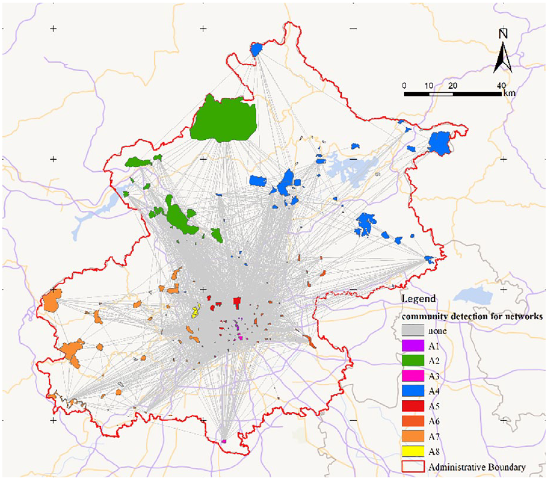
Community detection for scenic linkage networks.

The same algorithm was used to identify the community structure of the scenic networks of local and non-local tourists. The non-local scenic connection network is divided into eight communities with a modularity of 0.63, while the local scenic connection network is divided into eight communities with a modularity of 0.54. The modularity of both scenic networks demonstrates that community division is good. Some groups exhibit more evident spatial clustering links than others, as seen in Figure 8. Local tourists are divided into smaller groups than non-local tourists. The northwest Yanqi Lake group (A4), for example, is divided into two groups: the original Yanqi Lake (C6) and the eastern border. The largest scenic spot is also removed from the original group to join the Badaling group (C2). Simultaneously, some core-area scenic spots are united with peripheral scenic spots to form a new group, such as the Forbidden City–Tian Tan group (C3), as well as new group clusters.

Figure 8.

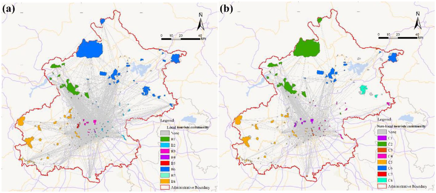
Community detection for scenic network. (a) Local and (b) Non-local.

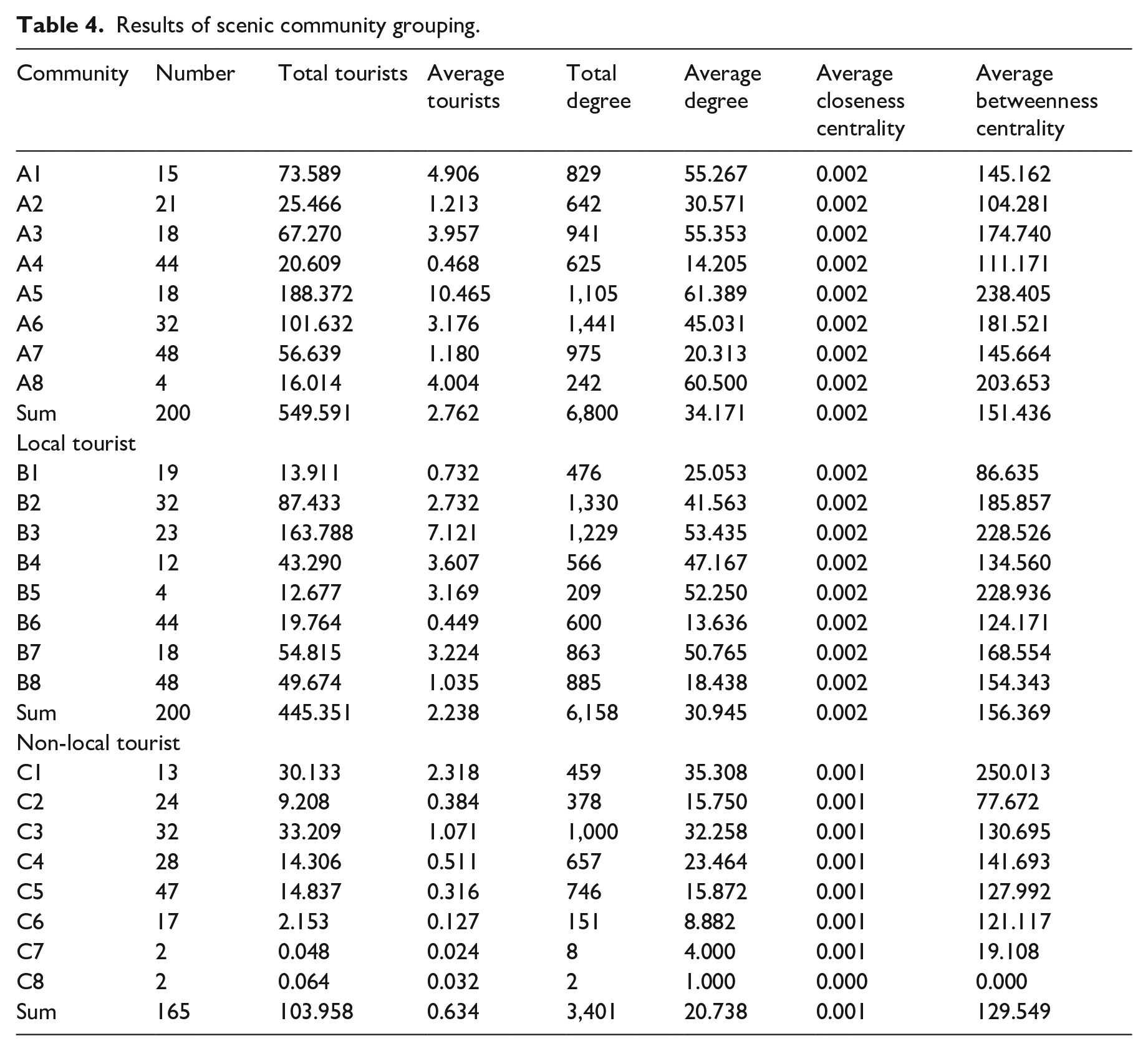
In terms of tourist volume and degree centrality of scenic spots within communities (Table 4), five of the eight communities formed by local tourists have above-average tourist volume and degree centrality (B2, B3, B4, B5, B7), while only two of the eight communities formed by non-local tourist contacts have above-average tourist volume (C1, C3) and only three have above-average degree centrality (C1, C3, C4). This suggests that the non-local tourists’ scenic spot network is more tightly connected to communities of core region scenic spots than the local tourists’ scenic spot connection network. This suggests that, when it comes to tourism management, greater thought should be given to spatial agglomeration for scenic spots targeted to attract non-local tourists, with significant clusters preserving convenient connections between them (e.g., C1, C3, and C4). Local tourists, on the other hand, need scenic spots to pay more attention to developing convenient internal linkages between clusters.

Table 4.

Results of scenic community grouping.

Community	Number	Total tourists	Average tourists	Total degree	Average degree	Average closeness centrality	Average betweenness centrality
A1	15	73.589	4.906	829	55.267	0.002	145.162
A2	21	25.466	1.213	642	30.571	0.002	104.281
A3	18	67.270	3.957	941	55.353	0.002	174.740
A4	44	20.609	0.468	625	14.205	0.002	111.171
A5	18	188.372	10.465	1,105	61.389	0.002	238.405
A6	32	101.632	3.176	1,441	45.031	0.002	181.521
A7	48	56.639	1.180	975	20.313	0.002	145.664
A8	4	16.014	4.004	242	60.500	0.002	203.653
Sum	200	549.591	2.762	6,800	34.171	0.002	151.436
Local tourist
B1	19	13.911	0.732	476	25.053	0.002	86.635
B2	32	87.433	2.732	1,330	41.563	0.002	185.857
B3	23	163.788	7.121	1,229	53.435	0.002	228.526
B4	12	43.290	3.607	566	47.167	0.002	134.560
B5	4	12.677	3.169	209	52.250	0.002	228.936
B6	44	19.764	0.449	600	13.636	0.002	124.171
B7	18	54.815	3.224	863	50.765	0.002	168.554
B8	48	49.674	1.035	885	18.438	0.002	154.343
Sum	200	445.351	2.238	6,158	30.945	0.002	156.369
Non-local tourist
C1	13	30.133	2.318	459	35.308	0.001	250.013
C2	24	9.208	0.384	378	15.750	0.001	77.672
C3	32	33.209	1.071	1,000	32.258	0.001	130.695
C4	28	14.306	0.511	657	23.464	0.001	141.693
C5	47	14.837	0.316	746	15.872	0.001	127.992
C6	17	2.153	0.127	151	8.882	0.001	121.117
C7	2	0.048	0.024	8	4.000	0.001	19.108
C8	2	0.064	0.032	2	1.000	0.000	0.000
Sum	165	103.958	0.634	3,401	20.738	0.001	129.549

Conclusion and discussion

This paper used several network analysis methods to investigate tourist movements and the key differences between local and non-local tourists. We applied the research method to a case study city, Beijing (China), and selected mobile phone data from Unicom as the data source to explore the spatial patterns of tourist flows. The conclusions can be summarized as follows:

(1) The Gini coefficients of total scenic spot tourists, non-local tourists, and local tourists are all high, showing that there is more disparity between scenic spots, and that non-local tourists have a more concentrated distribution than local tourists.

(2) Whether 5A scenic spots are significant in the models is determined by the regression findings of all regression models, all exhibiting positive effects. The category of scenic spots is also prominent in various models, but has a primarily negative impact. In addition, this study discovered that the number of subway stations within 500 meters has a significant impact on urban tourism attractions.

(3) The effect of distance decay on linkage is found to be considerable for total linkage, local tourists, and non-local tourists in general. When the linkage between scenic spots is separated into inside, outside and across the 6th Ring Road, however, the local connection of scenic spots across the 6th Ring Road is shown not to be associated with spatial distance.

(4) The whole tourist network can be divided into eight communities in terms of community division of the scenic spot linkage network. The scenic contact network for local tourists and the scenic spots for non-local tourists were both divided into eight communities, but the non-local tourist communities were more finely divided than the local tourist communities, with the majority of the scenic spots’ tourist volumes and linkage concentrated in a few communities.

The research structure can be applied to other case study sites. The study helps policymakers to better understand tourism differences from local and non-local tourists to improve the quality of tourism services for the benefit of the tourism industry. More consideration needs to be given to spatial agglomeration for scenic spots designed to attract non-local tourists, with convenient connections maintained between different clusters. For local tourists, on the other hand, scenic spots need to give more consideration to creating convenient internal connections within the clusters.

To undertake and attract more tourists, policymakers should emphasize the 5A scenic spots’ leading role, strengthen cooperation and complementarity between 5A scenic spots and neighboring scenic spots, improve the level of supporting facilities and tourism services, and create tourism clusters with shared facilities at the scenic spot level. Transit ties between significant scenic places and scenic clusters should be enhanced at the city level, and some tailored public transportation lines should be constructed to promote scenic spot accessibility.

Limitation

Our paper mainly had two limitations. Firstly, the research period of our study is 2020. The global COVID-19 pandemic in 2020 and lockdown policies affect global tourism, and also had a certain impact on the number and behavior of tourists in Beijing, which may cause limitations on our study. According to the Beijing Municipal Bureau of Culture and Tourism, the number of international tourists in Beijing in the fourth quarter of 2020 decreased by 90.6% compared to the same period in 2019, while the number of domestic tourists decreased by 8.6%. In this paper, we focused more on the domestic tourists to avoid this limitation as much as possible. Secondly, the measurement of transportation conditions in our paper was the number of subway stations within 500 and 1,000 meters. According to the Beijing Municipal Commission of Transport, the subway is the most important public transport mode. However, regardless of other transportation modes may cause limitations on detecting the travel patterns of tourists.

Footnotes

Declaration of conflicting interests

The author(s) declared no potential conflicts of interest with respect to the research, authorship, and/or publication of this article.

Funding

The author(s) disclosed receipt of the following financial support for the research, authorship, and/or publication of this article: This work was supported by The National Social Science Fund of China [No. 19BSH035].

Yang Xiao is an Associate Professor, Department of Urban Planning, College of Architecture and Urban Planning, Tongji University, China

Hang Wang is a Master’s student, Department of Urban Planning, College of Architecture and Urban Planning, Tongji University, China

Siyu Miao is a Phd student, Department of Urban Planning, College of Architecture and Urban Planning, Tongji University, China

Bo Xie is a Professor, School of Urban Design, Wuhan University, China

References

Ahas

Aasa

Mark

, et al. (2007) Seasonal tourism spaces in Estonia: Case study with mobile positioning data. Tourism Management 28(3): 898–910.

Ahas

Aasa

Roose

, et al. (2008) Evaluating passive mobile positioning data for tourism surveys: An Estonian case study. Tourism Management 29(3): 469–486.

Báez-Montenegro

Devesa-Fernández

(2017) Motivation, satisfaction and loyalty in the case of a film festival: Differences between local and non-local participants. Journal of Cultural Economics 41(2): 173–195.

Baggio

Scott

Cooper

(2010) Network science. Annals of Tourism Research 37(3): 802–827.

Brandes

(2001) A faster algorithm for betweenness centrality. The Journal of Mathematical Sociology 25(2): 163–177.

Casanueva

Gallego

García-Sánchez

M-R

(2014) Social network analysis in tourism. Current Issues in Tourism 19(12): 1190–1209.

Charles Chancellor

(2012) Applying travel pattern data to destination development and marketing decisions. Tourism Planning & Development 9(3): 321–332.

Chua

Servillo

Marcheggiani

, et al. (2016) Mapping Cilento: Using geotagged social media data to characterize tourist flows in southern Italy. Tourism Management 57: 295–310.

Clauset

Newman

Moore

(2004) Finding community structure in very large networks. Physical Review E 70(6 Pt 2): 066111.

10.

East

Osborne

Kemp

, et al. (2017) Combining GPS & survey data improves understanding of visitor behaviour. Tourism Management 61: 307–320.

11.

Freeman

(1978) Centrality in social networks conceptual clarification. Social Networks 1(3): 215–239.

12.

Gannon

Taheri

Croall

(2022) Memorable cultural consumption: Differences between local and non-local visitors to domestic sites. Journal of Hospitality and Tourism Insights 5(5): 842–864.

13.

García-Palomares

Gutiérrez

Mínguez

(2015) Identification of tourist hot spots based on social networks: A comparative analysis of European metropolises using photo-sharing services and GIS. Applied Geography 63: 408–417.

14.

Girardin

Calabrese

Fiore

, et al. (2008) Digital footprinting: Uncovering tourists with user-generated content. IEEE Pervasive Computing 7(4): 36–43.

15.

Grinberger

Shoval

(2018) Spatiotemporal contingencies in tourists’ intradiurnal mobility patterns. Journal of Travel Research 58(3): 512–530.

16.

Hickman

Chen

C-L

Chow

, et al. (2015) Improving interchanges in China: The experiential phenomenon. Journal of Transport Geography 42: 175–186.

17.

Hwang

Y-H

Gretzel

Fesenmaier

(2006) Multicity trip patterns. Annals of Tourism Research 33(4): 1057–1078.

18.

Javed

Younis

Latif

, et al. (2018) Community detection in networks: A multidisciplinary review. Journal of Network and Computer Applications 108: 87–111.

19.

Kang

Lee

Kim

, et al. (2018) Identifying the spatial structure of the tourist attraction system in South Korea using GIS and network analysis: An application of anchor-point theory. Journal of Destination Marketing & Management 9: 358–370.

20.

Kitchin

(2014) Big Data, new epistemologies and paradigm shifts. Big Data & Society 1(1). DOI: 10.1177/2053951714528481.

21.

Kuusik

Vadi

Tiru

, et al. (2011) Innovation in destination marketing. Baltic Journal of Management 6(3): 378–399.

22.

Leiper

(1979) The framework of tourism. Annals of Tourism Research 6(4): 390–407.

23.

Leung

Wang

, et al. (2012) A social network analysis of overseas tourist movement patterns in Beijing: The impact of the Olympic Games. International Journal of Tourism Research 14(5): 469–484.

24.

Lew

McKercher

(2006) Modeling tourist movements. Annals of Tourism Research 33(2): 403–423.

25.

Tang

, et al. (2018) Big data in tourism research: A literature review. Tourism Management 68: 301–323.

26.

Lindberg

Veisten

(2012) Local and non-local preferences for nature tourism facility development. Tourism Management Perspectives 4: 215–222.

27.

Liu

Huang

(2017) An application of network analysis on tourist attractions: The case of Xinjiang, China. Tourism Management 58: 132–141.

28.

McKercher

, et al. (2011) Tourism and online photography. Tourism Management 32(4): 725–731.

29.

Loi

Pearce

(2015) Exploring perceived tensions arising from tourist behaviors in a Chinese context. Journal of Travel & Tourism Marketing 32(1–2): 65–79.

30.

McKercher

Shoval

, et al. (2012) First and repeat visitor behaviour: GPS tracking and GIS analysis in Hong Kong. Tourism Geographies 14(1): 147–161.

31.

Mansfeld

(1990) Spatial patterns of international tourist flows—towards a theoretical framework. Progress in Human Geography 14(3): 372–390.

32.

Marine-Roig

Anton Clavé

(2015) Tourism analytics with massive user-generated content: A case study of Barcelona. Journal of Destination Marketing & Management 4(3): 162–172.

33.

Miah

Gammack

, et al. (2017) A big data analytics method for tourist behaviour analysis. Information & Management 54(6): 771–785.

34.

Mou

Yuan

Yang

, et al. (2020a) Exploring spatio-temporal changes of city inbound tourism flow: The case of Shanghai, China. Tourism Management 76: 103955.

35.

Mou

Zheng

Makkonen

, et al. (2020b) Tourists’ digital footprint: The spatial patterns of tourist flows in Qingdao, China. Tourism Management 81: 104151.

36.

Provenzano

Baggio

(2019) A complex network analysis of inbound tourism in Sicily. International Journal of Tourism Research 22(4): 391–402.

37.

Qin

Man

Wang

, et al. (2019) Applying big data analytics to monitor tourist flow for the scenic area operation management. Discrete Dynamics in Nature and Society 2019: 1–11.

38.

Raun

Ahas

Tiru

(2016) Measuring tourism destinations using mobile tracking data. Tourism Management 57: 202–212.

39.

Rodríguez

Martínez-Roget

González-Murias

(2018) Length of stay: Evidence from Santiago de Compostela. Annals of Tourism Research 68: 9–19.

40.

Shao

Huang

Wang

, et al. (2020) Evolution of international tourist flows from 1995 to 2018: A network analysis perspective. Tourism Management Perspectives 36: 100752.

41.

Shih

H-Y

(2006) Network characteristics of drive tourism destinations: An application of network analysis in tourism. Tourism Management 27(5): 1029–1039.

42.

Shoval

Ahas

(2016) The use of tracking technologies in tourism research: The first decade. Tourism Geographies 18(5): 587–606.

43.

Tiru

Kuusik

Lamp

M-L

, et al. (2010) LBS in marketing and tourism management: Measuring destination loyalty with mobile positioning data. Journal of Location Based Services 4(2): 120–140.

44.

Vanhoof

Hendrickx

Puussaar

, et al. (2017) Exploring the use of mobile phone data for domestic tourism trip analysis. Netcom 31–3/4: 335–372.

45.

Law

, et al. (2015) Exploring the travel behaviors of inbound tourists to Hong Kong using geotagged photos. Tourism Management 46: 222–232.

46.

World Travel and Tourism Council. (2020, June 20). Global Economic Impact Trends 2020. https://wttc.org/Portals/0/Documents/Reports/2020/Global%20Economic%20Impact%20Trends%202020.pdf?ver=2021-02-25-183118-360

47.

Xiang

Schwartz

Uysal

(2015) What types of hotels make their guests (un)happy? Text analytics of customer experiences in online reviews. In Tussyadiah

Inversini

(eds) Information and Communication Technologies in Tourism 2015. Cham, Switzerland: Springer, 33–45.

48.

Xiao-Ting

Bi-Hu

(2012) Intra-attraction tourist spatial-temporal behaviour patterns. Tourism Geographies 14(4): 625–645.

49.

Xing-zhu

Qun

(2014) Exploratory space-time analysis of inbound tourism flows to China cities. International Journal of Tourism Research 16(3): 303–312.

50.

Belyi

, et al. (2021) Characterizing destination networks through mobility traces of international tourists—A case study using a nationwide mobile positioning dataset. Tourism Management 82: 104195.

51.

Zou

Park

, et al. (2022) Understanding the movement predictability of international travelers using a nationwide mobile phone dataset collected in South Korea. Computers, Environment and Urban Systems 92: 101753.

52.

Yang

Algesheimer

Tessone

(2016) A comparative analysis of community detection algorithms on artificial networks. Scientific Reports 6: 30750.

53.

Zeng

(2018) Pattern of Chinese tourist flows in Japan: A Social Network Analysis perspective. Tourism Geographies 20(5): 810–832.

54.

Zeng

(2018) Factors influencing Chinese tourist flow in Japan—a grounded theory approach. Asia Pacific Journal of Tourism Research 24(1): 56–69.

55.

Zhao

Liu

, et al. (2018) Tourist movement patterns understanding from the perspective of travel party size using mobile tracking data: A case study of Xi’an, China. Tourism Management 69: 368–383.

56.

Zheng

Huang

(2017) Understanding the tourist mobility using GPS: Where is the next place? Tourism Management 59: 267–280.

57.

Zhou

Kimmons

(2015) Detecting tourism destinations using scalable geospatial analysis based on cloud computing platform. Computers, Environment and Urban Systems 54: 144–153.

A complex network analysis of local and non-local tourist flows in Beijing through mobile phone data

Abstract

Keywords

Introduction

Literature review

Study area and mobile phone dataset

Descriptive statistics of tourists

Centrality metrics in network analysis

Community detection in network analysis

Empirical analysis

Regional inequality of tourists

Pattern and centrality analysis of the tourism flow network

The associations of travel flow and attraction features

Scenic connection network and distance decay effect

Community detection of scenic linkage networks

Conclusion and discussion

Limitation

Footnotes

Declaration of conflicting interests

Funding

References