Sage Journals: Discover world-class research

Abstract

In experimental psychology, the term “pervasiveness” has been introduced to refer to the proportion of participants who exhibit an effect. This paper is a review of existing methods that could be used to extend the idea of pervasiveness to cross-sectional correlational data. More specifically, I consider how bivariate or multivariate effect sizes can be expressed or contextualized through proportions or percentages of individuals via the following methods: Kendall’s Tau, Common Language Effect Size indicators (Dunlap’s CLr, Li and Waisman’s B_P, Rosenthal and Rubin’s BESD and Mõttus’ TACT), rule-based methods (mostly Association Rule Mining, but Comparative Configural Models such as QCA and CORA are briefly discussed) and Observation Oriented Modeling. I illustrate the use of these methods in personality psychology using data from Soto's LOOPR project and highlight strengths and limitations for the different methods. I show that an Observed Percentage of Concordant Pairs (OPCP), easily obtained from Kendall’s Tau, can be used as a general-purpose common language effect size that also provides information on pervasiveness. The ‘pervasive’ R package, that provides the OPCP and information on a set of rules for use in a simple or multivariate regression setting, is introduced.

Keywords

pervasiveness clear language effect sizes association rule mining concordant pairs

Recently, Speelman and McGann (2020) introduced the concept of pervasiveness in the context of experimental psychology. Moore et al. (2023) transcribed the general idea of pervasiveness into a succinct question: “(…) how many people in the group observed in the experiment demonstrated the effect in their actual behaviour?” (p. 2). In other words, the basic idea of pervasiveness is to establish the proportion of participants who can be characterized by an effect. Considering the pervasiveness of an effect has advantages. For example, Grice et al. (2020) point out that pervasiveness can make evident some patterns that are obscured by sample-based statistics (also see Moore et al., 2023; Mõttus, 2022; Speelman & McGann, 2020 for further examples), that pervasiveness is easy to understand when compared to typical effect sizes (e.g., percentage of individuals meeting expectations vs percentage of shared variance, see Brooks et al., 2014 for an experimental paper empirically supporting this advantage of reporting effect sizes through proportions of individuals), and that pervasiveness can provide similar information across study contexts (for example, a percentage of individuals meeting expectations can be interpreted in the same way for experimental and correlational data).

In the case of within-individual experimental data, one can typically easily quantify the proportion of persons in the sample that exhibit the expected effect vs not (e.g., X% of participants responded faster in an experimental condition meant to foster a rapid response than in a control condition). However, as Speelman and McGann (2020) and Moore et al. (2023) acknowledge, alternative approaches are necessary for designs that yield single data points for individuals (these authors suggest Grice’s [2011] Observation Oriented Modeling [OOM] framework), as these designs preclude examining patterns within persons. In the case of between groups data, McGraw and Wong (1992) proposed the original “Clear Language Effect Size”, whereby one can estimate the probability that a person from a group has a higher value for a variable than a person from another group (for example, the probability that a man is taller than a woman given distributions of height for samples of men and women). Ruscio and colleagues (e.g., Ortelli & Ruscio, 2022; Ruscio & Mullen, 2012) provide more information (and analytical tools) for options to quantify the probability of superiority of members of a group vs another for a variable. In the case of cross-sectional correlational data with continuous variables, many approaches can be applicable to analogous questions on the pervasiveness of an effect. However, I am not aware of a review that presents these approaches together whilst providing researchers with information on their strengths and limitations.

As such, the goal of this paper is to explore and integrate various methodological approaches for pervasiveness analyses that may be applicable to a between-person correlational study design. This review was in part inspired by Mõttus (2022), who, as indicated by the title of their paper, spoke of “What Correlations Mean for Individual People”. One of their findings suggests that we should avoid stating that a high score on one variable implies a high score on a second variable in the presence of a correlation lower than .4. This recommendation is based on the fact that trisecting two normally distributed variables into three bins only results in over 50% of overlap between the “high” categories when correlations are over .4. Building on this, the present paper reviews an array of methods to inform what correlations (and correlation-like) effects imply for individuals.

The methods discussed include Kendall’s Tau (1938), Common Language Effect Size indicators (CLES) such as Dunlap’s (1994) CLr, the Binomial Effect Size Display (BESD) by Rosenthal and Rubin (1982), Trisect And CrossTabulate (TACT) by Mõttus (2022), rule-based methods such as association rule mining (Agrawal et al., 1993; Configural Comparative Methods such as Qualitative Comparative Analysis [QCA] and COmbinational Regularity Analysis [CORA] are also briefly discussed), and the OOM framework (Grice, 2011). While these methods vary in their assumptions and data requirements, they share the common goal of illustrating the presence of effects at the individual level rather than at an aggregated sample level.

Reflecting the advantages to pervasiveness analyses mentioned above, I will mostly discuss the strengths and limitations of the different approaches in terms of clear language effect sizes and data exploration capabilities. Because correlational studies often go beyond bivariate relationships, I also consider the multivariate capabilities of the methods where applicable.

The structure of the paper is as follows. In the next section, I will introduce a dataset from the LOOPR project (Soto, 2019), which will be used to illustrate the various methods under review. Following that, I will review several methods that can provide information on pervasiveness of effects at the individual level in the context of personality psychology. In the discussion, I provide an integration of the advantages and limitations of selected methods and showcase an R function that produces some pervasiveness information relevant to simple and multivariate regression.

As a final note at the onset of this paper, it is worth mentioning that the label of “pervasiveness” is newer than most of the methods I review. The authors of the methods I selected as relevant would not necessarily identify their methods as members of the class of “pervasiveness” analyses. I adopt the label of pervasiveness proposed by Speelman and McGann (2020) because I find it succinctly evokes the idea of frequency of effects at the individual level.

Some Information on the Applied Example

To illustrate the methods I will review, I examine the relationship between extraversion and positive affect in the LOOPR dataset provided by Soto (2019) here: https://osf.io/crk92. Analyses were not preregistered. For those methods requiring a bivariate relationship, I chose extraversion and positive affect as variables because their association is well-established (e.g., Lucas et al., 2008). Where relevant, I include the other Big Five traits as additional predictors. Supplemental materials, including code for all analyses for this paper, except those conducted on the OOM software, are presented here: https://osf.io/zm5f9/.

Positive affect was assessed with the Affect Balance Scale (Bradburn, 1969) with five yes (scored 2) or no (scored 1) items. A sample item is “During the past few weeks, did you feel…” “On top of the world?”. Cronbach’s alpha was .68. Scores are made by averaging the five items, such that scores range from 1 to 2. Some participants had missing data on positive affect: 26 participants missed one item, 1 participant missed 2, 1 missed 4, and 1 missed all 5. I removed the participants that missed 4 and 5 positive affect items (the final sample size is 3,107). For the others, their scores represent the average of the items to which they responded, using no imputation for missing values.

The Big Five personality traits were assessed with the BFI-2 (Soto & John, 2017) with twelve items each (60 total). Answers are provided on 1 to 5 Likert scales. A sample item for extraversion is “I am someone who… - Is outgoing, sociable”. Cronbach’s alphas range from .79 (agreeableness) to .89 (negative emotionality). Scores are made by averaging the scale items (reversing items where necessary), such that scores range from 1 to 5. The data set presents no missing values for the personality variables.

The correlations between variables are reported in Table 1 (along with the Observed Percentage of Concordant Pairs between variables, to be discussed later). As shown in this table, the correlation between extraversion and positive affect, the main relationship of interest, is of .37. The R-squared value is therefore .14 (rounded up).

Table 1.

Means, Standard Deviations, Correlations, and Observed Percentage of Concordant Pairs Between Study Variables

	M	SD	1	2	3	4	5	6
1. Extraversion	3.19	0.72	—	59.66	63.95	33.37	63.52	63.61
2. Agreeableness	3.71	0.63	.28**	—	68.86	35.98	62.59	57.79
3. Conscientiousness	3.73	0.72	.41**	.51**	—	33.13	59.93	59.36
4. Negative emotionality	2.87	0.88	−.49**	−.40**	−.48**	—	45.05	37.53
5. Open mindedness	3.69	0.66	.40**	.34**	.28**	−.15**	—	57.97
6. Positive affect	1.65	0.30	.37**	.21**	.25**	−.34**	.23**	—

Note. Pearson’s r are presented below the diagonal, Observed Percentage of Concordant Pairs above. The latter statistic is a linear re-expression of Kendall’s Tau and represents the percentage of pairs of participants where the person with the largest value on a variable also has the larger value on the other variable, with an adjustment for ties. *p < .05. **p < .01. This kind of table can be produced by the OPCP_mat() function of the ‘pervasive’ R package presented in the discussion.

The scatterplot presented at Figure 1, prepared with the flexplot R package (Fife, 2022), shows that positive affect is distributed on a rather sparse continuum. The Loess line of best fit appears slightly curved. A linear model including a squared extraversion term shows a statistically significant squared term (β = −.02, p < .01), but the total R-squared remains .14 (rounded down). The relationship appears to be mostly captured by a linear model.

Figure 1.

Scatterplot and Loess Line of the Association Between Extraversion and Positive Affect Produced by Flexplot

Kendall’s Tau and the Observed Percentage of Concordant Pairs

Kendall’s (1938) Tau is a statistic that is calculated from concordant vs discordant pairs of observations. Once two variables are expressed through ranks, a pair of participants i and j is deemed to be concordant with regards to variables x and y when x_i – x_j and y_i – y_j have the same valence. For example, suppose participant i ranks first on extraversion and positive affect (such that x_i = y_i = 1), and that person j ranks second on both variables (such that x_j = y_j = 2). Participants i and j would be a concordant pair because both x_i – x_j and y_i – y_j are both negative. A conceptual equation for Kendall’s Tau is given by equation (1). The fact that Kendall’s Tau is calculated on ranks enables the use of the statistic when two variables are on different scales (in fact, all the methods we review can be used with variables assessed on different scales, either because of transformations into ranks, standardization, or binning).

((number of concordant pairs) - (number of discordant pairs)) / (total number of pairs)

(1)

Tau can take values between −1 and 1, where 1 means that all possible pairs are concordant and 0 means that 50% of pairs are concordant and 50% of pairs are discordant. Note that in the typical application of Kendall’s Tau (“Tau-b”), the denominator is adjusted for ties.¹ The version of Kendall’s Tau using equation (1) (“Tau-a”) is actually rarely used. I will only use Tau-b in this paper. When data can be assumed normal, the expected value of r can be computed from Kendall’s Tau (e.g., Gilpin, 1993).

A convenient consequence of equation (1) is that Tau can be re-expressed to indicate the observed proportion of concordant pairs by dividing the value by two and adding .5 (multiply by 100 for percentage). This re-expression follows naturally from Kendall (1938), and other researchers have referred directly to this re-expression (e.g., Mastrich & Hernandez, 2021). However, I have not been able to find a commonly adopted name for this simple statistic. At the risk of contributing to jingle-jangle in the psychometric nomenclature, I will refer to the re-expression of Kendall’s Tau into a percentage as OPCP, for “Observed Percentage (or Proportion) of Concordant Pairs”. OPCP is very much related with concordance rates (also known as c-statistics or the area under the Receiver Operating Characteristic curve) from the realm of classification methods but differs namely in how ties are treated. Concordance rates include a weight of .5 to ties, whereas OPCP adjusts for ties as per Kendall’s Tau-b. In our applied example, the value of Tau is .27 and the OPCP is .64.

As a pervasiveness score, OPCP probably has an edge over Tau by virtue of being on a more familiar metric (percentage or proportion vs −1 to 1 index). A notable advantage of Tau and OPCP over most of the methods to be covered in this review is that there is no need to bin the data at all. In terms of limitations, Tau and OPCP are not particularly informative for data exploration, being a simple indicator of monotonicity. Moreover, Tau and OPCP are restricted to the bivariate use-case. One could provide the OPCP between an outcome and the predicted outcome based on a multivariate model as a supplement to an R-squared value in a multiple regression, but this does not elucidate the role of individual variables (neither does the R-squared, to be clear). With regards to our applied example, a multiple regression model with all Big Five traits predicting positive affect produces an R-squared of .18 and an OPCP of .66 (three traits have significant coefficients: extraversion, negative emotionality, and open mindedness).

Common Language Effect Size Indicators

Common Language Effect Size (CLES) indices tend to be almost, but not quite, indicators of pervasiveness. In fact, instead of expressing the pervasiveness of an effect in a given dataset, most CLES express how pervasive we should expect an effect to be under normal circumstances (i.e., when both variables are normally distributed). As Zhang (2018) points out, these expected values might be better at representing population parameters than observed (or “empirical”) values are. However, expected values do not present the proportions that are actually in the data and those that are based on Pearson’s r rely on assumptions such as normality and linearity. Mastrich and Hernandez (2021) provide a review of CLES indices, three of which are relevant to our context.

The first is Dunlap’s (1994) extension of McGraw and Wong’s (1992) discrete groups CLES to continuous variables. “It is simply the probability that if a first randomly selected individual has a higher score than a second randomly selected individual on the first variable, the first individual will also have a higher score on the second variable.” (Dunlap, 1994, p. 510). The conceptual link to OPCP is evident from this definition. Dunlap (1994) proposes the formula presented in equation (2).

{CL}_{R} = \arcsin (r) / π + . 5

(2)

Dunlap’s CL_R and OPCP approximate each other when normality can be assumed. To demonstrate this, in supplemental materials, I provide a simulation of 1000 samples each with n = 1000. This simulation included normally distributed variables with varying degrees of correlation. Pearsons’ correlation coefficient between Dunlap’s CLES and OPCP across simulations was r = .99, suggesting near-perfect monotonicity. As such, Dunlap’s CL_R can be understood to represent the expected value of OPCP under normality (the term “observed” in “Observed Proportion of Concordant Pairs” is meant to contrast with the fact that Dunlap’s CL_R reflects the expected proportion of concordant pairs). In Figure 2, I plot the expected values of OPCP (i.e., values of CL_R) against values of r ranging from 0 to 1. Note that the slope of the curve at r = .2 (a median correlation in personality psychology, Gignac & Szodorai, 2016) is of only .32. This means that we should expect OPCP to increase quite a bit slower than r over the range of most personality psychology effect sizes.

Figure 2.

Expected Values of OPCP (=CL_R) as a Function of r Note. The y-Axis Starts at .5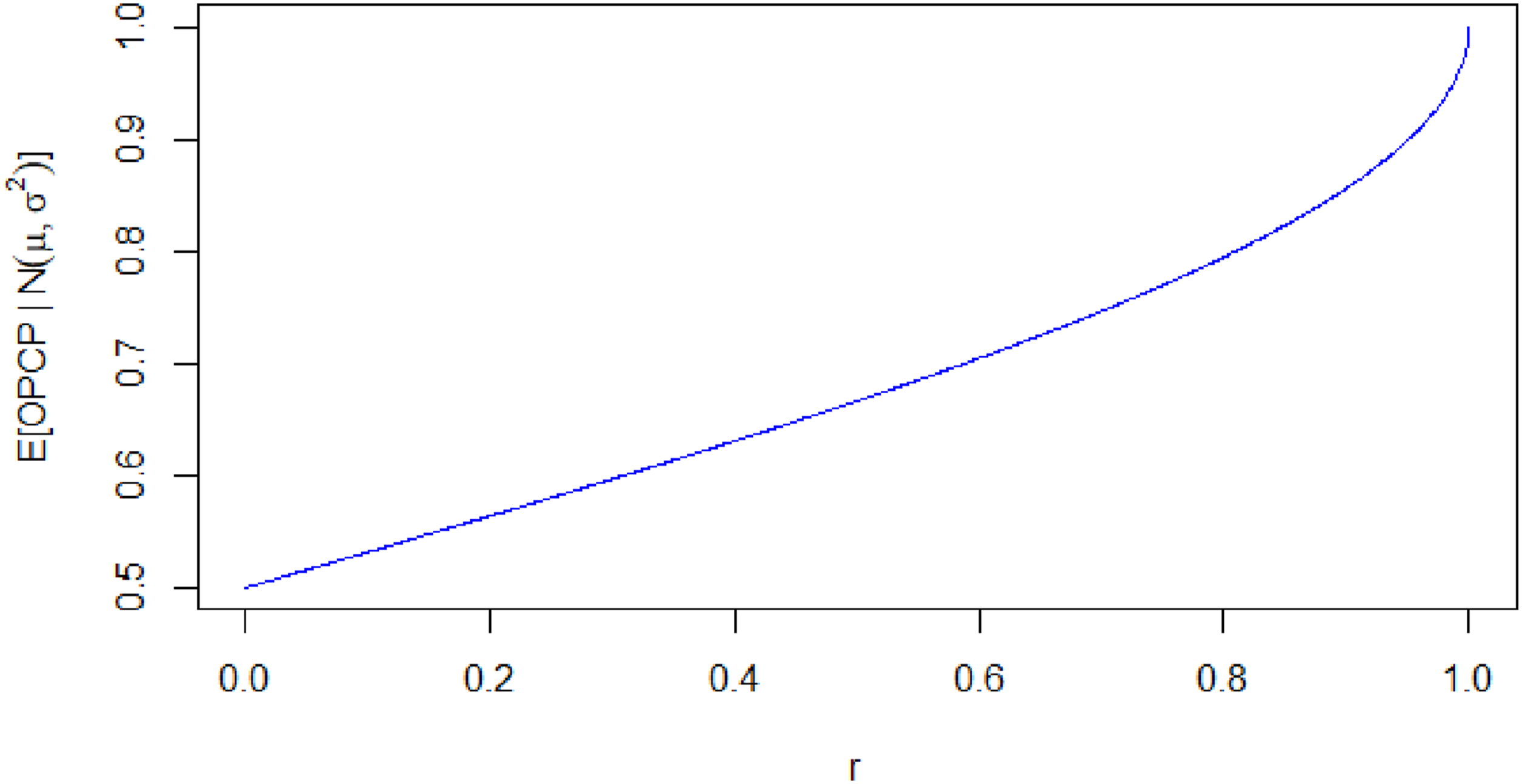

The second CLES reviewed by Mastrich and Hernandez (2021) is Li and Waisman’s (2019) CLES for nonparametric bivariate relationships, called probability of bivariate superiority (PBS, also denoted B_P). It represents the probability that a person with a score higher than the sample mean on a variable will also score higher than the mean on another variable. For example, the mean of extraversion, reported in Table 1, is 3.19 and the mean of positive affect is 1.65. The value of B_p in this instance is 63.41. This value represents the percentage of participants with extraversion scores higher than 3.19 who also have a score higher than 1.65 on positive affect.

Unlike Dunlap’s (1994) CL_R, Li and Waisman’s (2019) B_p does provide information on the actual observed data. However, Mastrich and Hernandez (2021) point out that Li and Waisman’s B_P, like Dunlap’s CL_R, tends to correlate with OPCP at near-perfect levels. Nevertheless, because B_P is based on the mean, it may differ from OPCP when large outliers are present. Take for example two arbitrary variables x and y with five participants each, x^T = [1, 2, 1, 2, 10] and y^T = [2, 1, 2, 1, 10]. Both x and y have means of 3.2. In this scenario, B_p = 1 because 100% of the cases above the mean on x are also above the mean on y (here, this refers to the single participant with a value of 10 for both variables). On the other hand, OPCP = .5 because the relationship is not monotonic. As Li and Waisman (2019) point out, B_P is not a monotonicity index.

The third is Rosenthal and Rubin’s (1982) BESD. This is the first index we discuss that does not summarize a relationship with a single number. Instead, the BESD provides a cross-tabulated 2 × 2 grid where cells present the proportion of high or low values for an outcome variable based on high or low values of a predictor. A typical formula given for BESD is that the proportion in the cells on the diagonal is r/2 +.5, with the off diagonal obtained by subtracting the resultant value from 1. However, the original formulation of the BESD supposed binary variables. As pointed out by Mõttus (2022), the typical formula does not correct for information loss due to dichotomization when variables are continuous. This results in inflated values if a BESD is made using median-split continuous variables. The TACT package (Mõttus, 2022) provides a modified approach to creating a BESD that corrects this behaviour by cross-tabulating median-split data. In the case of median-split normal data, the high-high cell is by definition equivalent to Li and Waisman’s (2019) B_P, and consequently to OPCP. A TACT-BESD for a correlation of .37 is presented in Figure 3(a).

Figure 3.

TACT-BESD and TACT for a Pearson Correlation of .37

A final evolution of CLES that should be discussed is TACT by Mõttus (2022). While the TACT package can be used to produce a BESD, its main function is to “Trisect And Cross-Tabulate”. In fact, an important take-away message from Mõttus (2022) is that it is preferable to trichotomize rather than dichotomize variables. This is namely because the former practice allows one to examine the behaviour of the “middle” of the distribution, which can be strikingly different from what happens at the ends of the distribution. For instance, with a .37 correlation, the high-high cell in a TACT display (see Figure 3(b)) suggests that 48.8% of participants who are high in extraversion are also high in positive affect, whereas only 35.5% of medium extraversion participants show medium levels of positive affect. In addition to a trisection and crosstabulation of generated normal data, TACT can also provide a display for user-provided observations. However, even in this case TACT does not provide an actual representation of pervasiveness because it “harmonizes” the grid (i.e., it imposes symmetry), for example by averaging out the high-high and low-low cells.

Overall, this review of CLES indices suggests that the OPCP value can produce a pervasiveness index that is quite coherent with existing practices – to the point of indicating potential jingle-jangle issues – but with the added value of representing actual data. As a whole, CLES are characterized by being limited to the bivariate use-case. While TACT can produce a scatterplot that is useful for data exploration, its main advantage with regards to pervasiveness might be its ability to let us understand that expectations should be different between the ends of the distribution and the middle.

Rule-Based Methods

The goal of rule-based methods is, stated simply, to find configurations of categories that frequently co-occur. For example, based on the correlation between extraversion and positive affect, one might suppose that the categories of “low extraversion” and “low positive affect” should frequently co-occur (likewise for high and high values). Because rule-based methods work on categorical data, researchers with continuous data must bin their variables before proceeding to the analysis (binning will be discussed with more depth in the following section). Rules are typically reported in a shape consistent with the following example:

{Extraversion = Low = > PositiveAffect = Low}

Predictors are presented on the left-hand side and outcomes on the right-hand side. Different rule-based methods adopt various indicators to provide information on the pervasiveness of the rules.

The rule-based methods I discuss mostly emerge from two distinct traditions. Association rule mining emerges from computer science (Agrawal et al., 1993) and is traditionally applied in the commercial space (e.g., to study shopping habits such as which items are frequently sold together). Comparative Configural Models such as QCA and CORA are based on algorithms from electronic engineering and were introduced to the social sciences via sociology and political sciences (e.g., Ragin, 1987). One contribution from the psychometric literature that has many similarities to the rules-based methods I discuss is Configural Frequency Analysis (see Stemmler, 2020; von Eye & Wiedermann, 2022 for recent treatments). However, I opted not to review Configural Frequency Analysis in depth because its ultimate concern appears to be the statistical significance of the frequency of configurations, rather than the pervasiveness of configurations per se.

Association Rule Mining

Association rule mining, also called association analysis or frequent itemset mining, attempts to discover interesting patterns in (typically) large datasets (see Tan et al. (2018), for an introduction and Fournier-Viger et al. (2017) for an in-depth review). An important advantage of association rule mining is its ability to handle large volumes of data and variables. In this sense, an interesting use for association rule mining is to provide contextualizing information for multivariate effects. For instance, earlier, I reported that three personality traits (extraversion, negative emotionality, and open mindedness) have statistically significant terms when positive affect is regressed on the Big Five. Association rule mining can indicate how frequently high extraversion, low negative emotionality and high open mindedness occur in a dataset, how frequently people with that configuration of personality traits also report high positive affect, and how that last proportion compares with the base-rate of high positive affect in the sample.

In other words, association rule mining can indicate how pervasive the pattern suggested by a regression model is. One can further expand this use for a wider exploratory purpose, for instance by including more variables. Indeed, it is possible to run an item-level analysis of associations, should a researcher have a question relevant to that level (the risk then is in generating a very large volume of association rules, as we will see). A discussion of the advantages and limitations of association rule mining requires some familiarity with how the analysis is conducted. For this reason, a quick overview of the steps required for association rule mining follows.

The first step that a typical personality researcher will face when using rule-based methods is binning their continuous variables. Now, it is well-established that binning is generally a bad idea (e.g., Cohen, 1983). It reduces statistical power by restricting variance and it introduces arbitrary cutoffs that separate data-points which are in reality close to one another. Moreover, choosing different cutoffs for bins is likely to produce different outcomes in analyses. On the other hand, in consideration of the fact that a goal of pervasiveness analyses is to find information that is different from what one might find with our usual methods, one can indeed find data exploration methods based on pervasiveness if one can accept the limitations inherent to binning. Moreover, binning may also be an occasion to meaningfully engage with one’s data. For example, attempting to define what one considers high and low values for a trait imposes reflections on how we make sense from personality scores, among others (e.g., Grice et al., 2020).

In traditional applications of association rule mining, data must be binary. Therefore, each bin should be coded as a single column. For example, if extraversion is trisected, a person with a high level of extraversion should have a 0 for low extraversion, 0 for medium extraversion, and a 1 for high extraversion. When binning, the researcher will face two main decisions: the number of bins to keep and reasonable cutoffs for bins. With regards to the number of bins, an important consideration is the risk of sparse configurations. Having very fine-grained categories can lead to very small number of cases in each configuration. Therefore, it may be generally preferable to opt for a small number of bins. Considering Mõttus’ (2022) arguments for trisecting over bisecting, I will illustrate association rule mining with trichotomized variables.

With regards to cutoffs for bins, different strategies exist. We can cut on n-tile values (e.g., the median or on tertiles), we can adopt a frequency approach that attempts to make group memberships as equal as possible (this approach can be different from n-tiles when there are ties in the data), we can create clusters (for example by k-means clustering), or we could choose substantive cutoffs based on the assessment scale (for example, on scores created from 5-point Likert items, we might decide that an average of at least 4 warrants binning in the high group and of maximum 2 in the low group, with participants between those scores being medium). There may be advantages to different approaches in different contexts, but I am not aware of strong arguments for a particular method in the general case. Because binning strategy will influence results, a multiverse approach (e.g., Steegen et al., 2016) in such analyses may be advantageous. In any event, it is likely advisable to look at the distribution of the data to determine if some cutoffs appear to be more reasonable than others.

For our applied example, I used the frequency approach. I used the discretize function of the arules package (Hahsler et al., 2005) to trichotomize all variables. The cut-offs for each variable and the frequency of the bins are reported in Table 2. We can see from this table that the discretize function was not able to create perfectly equal groups, particularly for positive affect. Furthermore, the cut-offs do not necessarily match an intuitive interpretation of “high”, “medium” and “low” scores. For example, a score of 4 on conscientiousness implies that a person mostly agrees with items presenting conscientiousness content, but this score is classified as medium. In a similar way, a score of 3.3 is high for negative emotionality but low for conscientiousness.

Table 2.

Results of Trisection for Association Rule Mining

	Cutoffs	N low (%)	N medium (%)	N high (%)
Extraversion	2.92; 3.5	1028 (33.09)	985 (31.7)	1094 (35.21)
Agreeableness	3.42; 4	957 (30.8)	1024 (32.96)	1126 (36.24)
Conscientiousness	3.33; 4.08	938 (30.19)	1055 (33.96)	1114 (35.85)
Negative emotionality	2.5, 3.25	1028 (33.09)	988 (31.8)	1091 (35.11)
Open mindedness	3.33, 4	916 (29.48)	1089 (35.05)	1102 (35.47)
Positive affect	1.6; 1.8	891 (28.68)	690 (22.21)	1526 (49.11)

After binning, the researcher can proceed to the analysis, and then to selecting interesting patterns. When running the analysis, the analyst must indicate a minimum level of “support”, or frequency of appearance in the data (i.e., a minimum level of pervasiveness), for the rules to be retained. I am not aware of literature specific to association rule mining on selecting an appropriate minimum support threshold. The idea is to set this threshold high enough to avoid the risk of “producing fancy configurations based on almost no data.” (Borg et al., 2018, p. 49),², but low enough to not miss interesting associations.

Using the arules package (Hahsler et al., 2005), I pulled rules where the Big Five personality variables were on the left-hand side (LHS), positive affect levels were on the right-hand side (RHS), and I specified a minimum support of 3%. In our applied example, 3% of 3,107 is rounded up to 94 individuals. Of course, this implies that rules related to medium positive affect, a category reflecting only 22.21% of the sample, are rather less likely to obtain support than rules for high positive affect (49.11% of individuals in the sample) regardless of the issue of lower predictability with medium values.

In Table 3, I report the rules with the highest “lift” for each level of positive affect. Lift is defined as P(RHS|LHS)/P(RHS), or as the “confidence” of the RHS permitted by a rule divided by the support for the RHS (see note below Table 3). When lift is higher than 1, P(RHS|LHS) > P(RHS), such that the rule is associated with an increase in the occurrence of the outcome compared to the base rate.

Table 3.

Association Rule Mining Results Between Big 5 Traits and Positive Affect

RHS	LHS with highest lift	Support	Coverage	Confidence	Lift
Low positive affect	{Extraversion = Low,	.04	.07	.60	2.09
Low positive affect	NegativeEmotionality = High, OpenMindedness = Low}	.04	.07	.60	2.09
Medium positive affect	{NegativeEmotionality = High,	.04	.12	.30	1.34
Medium positive affect	OpenMindedness = High}	.04	.12	.30	1.34
High positive affect	{Extraversion = High,	.06	.07	.82	1.67
	Agreeableness = High,
	Conscientiousness = High,
	NegativeEmotionality = Low,
	OpenMindedness = High}

Note. LHS refers to left-hand side, or the predicting categories. RHS refers to right-hand side, or the outcome categories. Support is the proportion of participants with the pattern suggested by the LHS and RHS; Coverage is the proportion of participants with the pattern suggested by the LHS only; Confidence is the proportion of participants with the LHS that also show the RHS; Lift is the increase in confidence in the RHS permitted by the LHS.

Table 3 illustrates how association rule mining might be used to explore a dataset. In line with our multiple regression, low levels of extraversion and open mindedness and high levels of negative emotionality is indeed the pattern of results most notably associated with low levels of positive affect. In terms of pervasiveness, we learn from this table that this configuration of personality traits occurs in 7% of participants (coverage) and that 60% of these people report low levels of positive affect (confidence). Interestingly, the rule with the highest lift for high positive affect is not simply the reverse of the rule we just reviewed. Agreeableness and conscientiousness are added to the high positive affect rule. The interested researcher may wish to investigate the presence of heteroskedasticity or non-linear effect with regards to these two predictors. The confidence for this rule is higher than the confidence for low positive affect, but the lift is lower.³

The medium positive affect rule has lower lift than the other two rules. This is in line with Mõttus’ (2022) comments on lower prediction capacity in the middle of distributions, and another demonstration of the added nuance provided by trisection. Another observation about the medium positive affect rule is that the best rule to predict medium positive affect includes terms that were also in the low and high positive affect rules. Here, a “paradoxical” combination of high negative emotionality and high openness is the rule with the highest lift for medium affect; medium levels of personality traits do not appear to figure in the best combination to predict medium affect.

Overall, association rule mining allows for contributions to both of the main motives for pervasiveness. It provides clear language effect sizes. For example, the fact that 7% of the sample display the configuration suggested by the multiple regression for the prediction of low positive affect and that 60% of these people indeed do report low positive affect provides clear context for the regression. In terms of data exploration, it can also provide some nuances that are not obvious from a regression. Here, we might wonder why the combination that is most predictive of high positive affect in association rule mining is not simply the mirror reflection of the low positive affect configuration. One might explore potential issues of non-linearity and heteroskedasticity based on this information. Moreover, association rule mining has the advantage of allowing many predictor variables (in supplemental materials, I show the results of association rule mining with all 60 items from the BFI-2 at once – the rule with the highest lift for high positive affect includes the items “Is outgoing, sociable.”, “Is relaxed, handles stress well.”, “Stays optimistic after experiencing a setback.”, and “Tends to feel depressed, blue”, in the expected valence).

On the other hand, association rule mining can produce an unwieldy amount of information (e.g., the item-level analysis produced 87,215 rules with 3% support). While I focused only on the rules with the highest lift to keep things simple, there may be any number of interesting or relevant rules. Furthermore, skew makes for some awkwardness when binning. Insofar as items for a personality trait questionnaire can be seen as a sample from a universe of items relevant to a personality trait, it may not be unreasonable to suppose that skew could be a result of sampling variability in both the participant and item samples, with the mean (and skew) being seen as essentially arbitrary. But it remains somewhat questionable to classify someone as low agreeableness when they mostly agree with the agreeableness content to which they responded (and this is besides the possibility that skew in personality trait scores could be the result of the semantic content of items (e.g., Arnulf et al., 2024) and issues in the use of Likert scales to “measure” traits (Uher, 2022)). Incidentally, trisecting based on substantive interpretations of Likert scales would only produce the reverse of these issues; very few participants would be classified as low agreeableness if a cutoff of 2 was used for low agreeableness (and therefore very few rules using low agreeableness could meet support cutoffs).

Comparative Configurational Models

Approaches related to association rule mining also deserve some comments. For example, the family of models called Comparative Configural Models (e.g., Thiem, 2024), including Qualitative Comparative Analysis (QCA), Coincidence Analysis and COmbinational Regularity Analysis (CORA), aim to reduce rule sets to those rules that are minimally sufficient to cover the causal paths between inputs (predictors) and outputs (outcomes) via Boolean algebra. Researchers can indicate a minimum frequency (i.e., “support” in the association rule mining lingo) with which a configuration must appear in a dataset to be considered, and results include statistics to indicate the pervasiveness of selected rules. These methods were originally conceived for small-n research (e.g. Ragin, 1987), but they indeed can be made to run with a larger dataset (e.g., Rutten, 2022). To the best of my knowledge, no mainstream personality journal has published a paper using CCMs, although studies using CCMs, specifically QCA, with personality variables can be found.

The application of CCMs to personality data is questionable for a few reasons, some of which follow. First, CCMs can be computationally demanding (to the point of non-convergence in a practical timeframe) when datasets with many columns and rows are used, and minimized rule sets may still be quite complex under these conditions (Chiu & Xu, 2023). Second, CCMs are deterministic⁴ in their essence (e.g., Chiu & Xu, 2023) but personality processes should likely be considered probabilistic (for example based on the “Random Error Process” of the Whole Trait Theory by Fleeson & Jayawickreme, 2015). Third, in an attempt to palliate to the drawbacks of binning, researchers may be tempted to dichotomize their data using fuzzy sets (this was true of all papers I have found using QCA with Big Five personality data). Fuzzy sets are meant to be unipolar (Duşa, 2018, p. 111). Personality questionnaires assess traits on a bipolar continuum, such that interpretations from fuzzy sets may be not quite coherent with the data.

Insofar as researchers may still be interested in finding those rules that are both pervasive and minimally sufficient to predict an outcome, recent work in machine learning such as Bayesian Rule Sets (Wang et al., 2017) and Truly Unordered Rule Sets (Yang & van Leeuwen, 2023) offers heuristic approaches to reducing rule sets that may improve performance in a probabilistic many-variables-large-n context (Chiu & Xu, 2023). While Chiu and Xu (2023) provide an R package to help produce Bayesian Rule Sets, Truly Unordered Rule Sets, which perform better than Bayesian Rule Sets (according to Yang & van Leeuwen, 2023) are not yet released in a user-friendly documented package.⁵ Older methods such as those based on decision trees may also provide more limited rule sets. The issue here is that it is known that decision trees do not converge on optimal rule sets (e.g., James et al., 2023, p. 331), at least in part because of their “greedy” nature (i.e., all rules must include the first split).

CCMs and their machine learning counterparts provide interesting methods of inference that are deeply intertwined with pervasiveness. However, for the moment, it appears rule reduction methods are either not fully appropriate to the context of personality psychology, underperforming, or rather inaccessible. In this context, it may be sufficient for researchers wishing to augment the presentation of their results with pervasiveness information to select some specific patterns (say, the high and low patterns suggested by a multiple regression) and report support and confidence for these patterns. Motivated researchers could also contrast these patterns with the highest lift rules, as done above.

Observation Oriented Modeling

Observation Oriented Modeling is the name Grice (e.g., 2011) gives to their proposed analytical framework, which is entirely based on pervasiveness (again, the ideas predate the term). Grice (2011) outlines the philosophical and mathematical underpinnings of this approach. The approach endorses philosophical realism (essentially, reality exists and can be known), and analyses are conducted on the “deep structure” of observations. Deep structure refers to a way in which non-quantitative ordered observations may be coded. For example, a person answering a 5-point Likert scale with an answer of 4 would have an input of 00,010 entered into the analyses, and a person answering 3 would have an input of 00,100. In this way, the full information from an ordered response may be coded without assuming interval levels of measurements. Grice provides a free (proprietary) software for the purpose of executing OOM analyses (here: https://idiogrid.com/OOM/index.php/download/). Most of the analyses provided in the OOM software are better suited for the within person context, but some that are useful for between persons analyses are presented here.

Build/Test Model

In a simple bivariate case where one ordering (Grice’s preferred term for variables) is presumed to “cause” (or at the very least be an antecedent to) another ordering, Build/Test Model provides a crosstabulation of the two orderings. Figure 4 presents the graphical output from the model “Extraversion -> Positive Affect”. The numbers represent the column proportion, such that 66% of highly extraverted people report high positive affect (but keep in mind that 49% of participants were binned in the high positive affect category). In line with Mõttus’s (2022) comments on the value of trisection, we can see that the hit-rate for middle values is lower than for low or high values. We can see in Figure 4 that the Percent Correct Classifications (PCC) value is 46.06. This means that approximately 46% of participants are in matching bins for both orderings.

Figure 4.

Predicting Positive Affect From Extraversion: OOM Software Build/Test Model Results. Note. Numbers Represent Column Proportion (e.g., 66% of Participants With High Extraversion Reported High Positive Affect)

The OOM software provides a randomization test for the PCC value. For 1000 permutations, the values of one ordering are randomized, and the PCC is observed. The results of this randomization test are called the c-value. In the randomization test conducted in our applied example, the highest randomized PCC achieved was 36.72 and the c-value is reported as <.001 (i.e., in no case out of 1000 did the permutation produce a PCC greater than or equal to the observed PCC, but the c-value is not reported as “0” because an eventual permutation could produce such a value). In this context, it appears extraversion and positive affect bins match more frequently than might be expected by chance. Build/Test Models allows for other types of models, such as the analysis of conjunctions between levels of data. For example, in the online supplement, I share Figure S1 that allows examination of the relationship between extraversion and negative emotionality on the one hand and positive affect on the other.

Pattern Analysis (Crossed Orderings)

Pattern analysis allows a researcher to select expected combinations of values (for example, low-low, medium-medium, and high-high for extraversion and positive affect, see Figure 5) and to examine the frequency and chance value of these combinations. In that sense, this analysis can be considered an a priori version of the Build/Test Model we examined. Just like with Build/Test Model, the example pattern just cited covers 46.06% of the cases (c-value <.001 with maximum randomized PCC of 36.40). Different expected patterns can be explored. For example, knowing that middle values are less predictive, we might decide to select only low-low and high-high combinations. With these combinations, PCC is 37.98 (c-value <.001, maximum randomized PCC = 28.90). It appears that even if medium values are less reliable predictors than low and high values, their inclusion still improves the overall accuracy of the prediction without adding much noise. Likewise, noting that the diagonal only includes 46.06% of the data, a researcher might be tempted to instead predict that cases will actually fall off the diagonal. While the PCC is indeed higher with this prediction (53.94), the results show that this approach is misguided: 100% of permutations achieved a higher randomized PCC (c-value >.999, minimum randomized PCC = 63.57).

Figure 5.

Examples of Patterns Selected a Priori for Pattern Analysis (Crossed Orderings) in OOM. Note. The Highlighted Cells Indicate the Expected Patterns. The Cells Indicate Raw Frequencies (e.g., 720 Individuals Have High Extraversion and Positive Affect Values)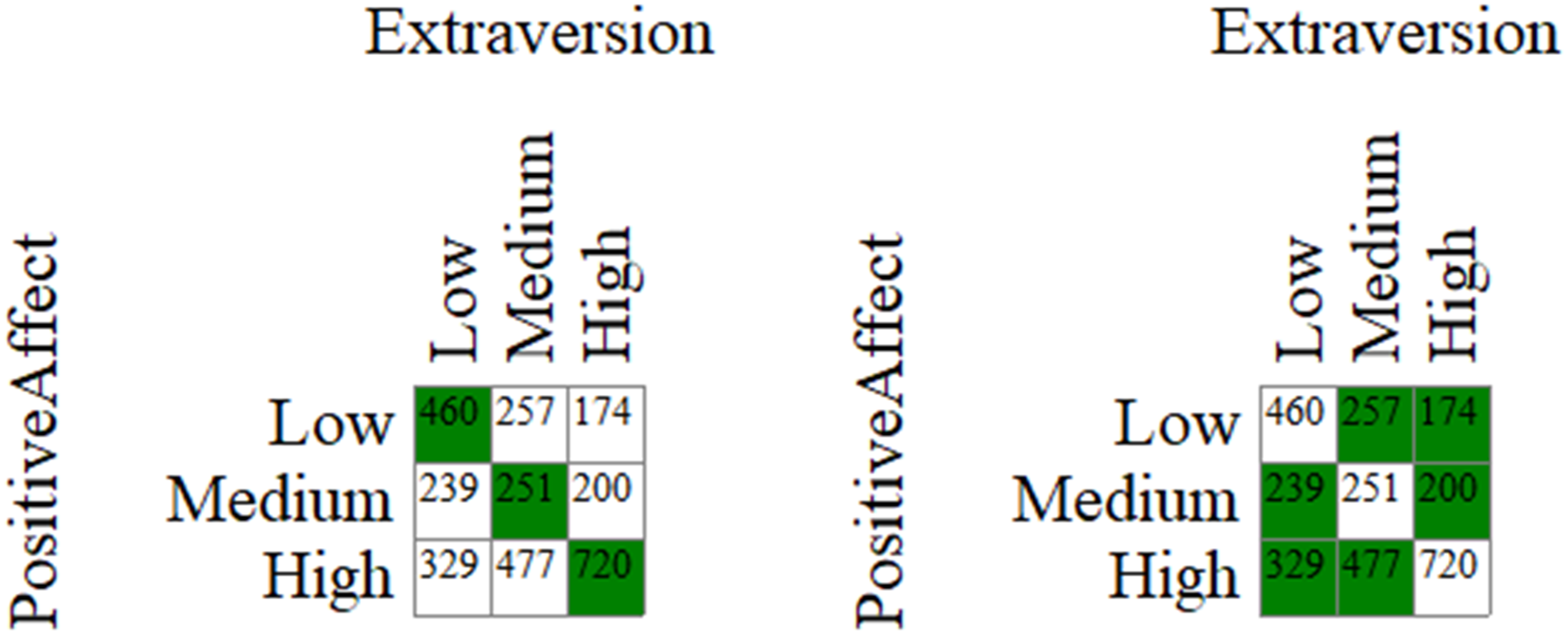

Ordinal Pattern Analysis (Crossed Orderings)

Ordinal pattern analysis with crossed orderings allows us to produce results that are not unlike Kendall’s Tau and the OPCP. Instead of being based directly on hit-rate like Build/Test Model and Pattern analysis (crossed orderings), this analysis examines whether those in a higher category of extraversion are indeed in a higher positive affect category. In this trisected dataset, those higher in extraversion were indeed in a higher positive affect category for 45.46% (c < .001) of participant pairs. It goes beyond summarizing a relationship with a single figure by examining the patterns for each category. For example, in our applied example, 52.93 % of high extraversion individuals are in a higher positive affect bin than low extraversion individuals, but this proportion is reduced to 44.33% when one compares the positive affect of middle and low extraversion individuals (all ties in the outcome are classified as “incorrect”, and there are many ties in the positive affect data), and to 38.71% when comparing high and middle extraversion individuals. All c-values are <.001, with the highest PCC values for the randomization tests respectively being 34.68, 34.80, and 35.84. In ordinal pattern analysis, binning is not strictly required if at least one of the orderings is somewhat coarse. For instance, in our case, there are only 10 different observed values for positive affect (there would only be six if we excluded all participants with any missing data). Positive affect can therefore be used as a grouping variable. Using this setup, the omnibus PCC (63.36%) approximates the OPCP (63.61%), with any difference resulting from the treatments of tied values.⁶ It becomes somewhat more intractable to examine the patterns for each category when the grouping variable has more than a few categories (there are n(n-1)/2 pairs of categories to compare in the general case, or 45 comparisons in the present case with 10 observed values).

Overall, OOM is an effective way of clearly communicating effect sizes and of exploring one’s data. It is more targeted in nature than association rule mining (the researcher has to select specific effects to look at), but it does provide more information than a single monotonicity index. It is generally affected by the same drawbacks of binning than other “hit-rate” methods (e.g., loss of information), but has the advantage of including visual support for many of its analyses and the randomization test is an informative approach to determine the “interestingness” of effects (for example, as an alternative to lift).

Discussion

In this paper, I reviewed different methods that can provide information on the pervasiveness of effects in a correlational, possibly multivariate, setting. Two general strategies appear to exist. The first is based on counting concordant pairs, and the second is based on “hit-rate” (i.e., the number of correct predictions). This second strategy is adopted by most of the methods reviewed. I showed that the OPCP, easily derived from Kendall’s Tau, is functionally equivalent to many CLES whilst avoiding assumptions such as normality and not misrepresenting proportions in the case of continuous variables (such as might be done with a traditional application of the BESD; Mõttus, 2022). Li and Waisman’s (2019) B_P can provide different information from the OPCP, but can also be conceived as equivalent to mean-split association rule mining between two variables. If trisection of data is to be preferred to dichotomization, association rule mining may be a better option. Nevertheless, I note that Li and Waisman’s (2019) code provides added value such as a 95% confidence interval for B_P. I discussed rule-based methods. I showed that the “confidence” of specific rules appears to be a straightforward path to discussing pervasiveness in a multivariate setting, but that challenges remain in the identification of interesting, reduced, rule sets. Finally, I discussed OOM, which is presented as a framework for quantitative research in psychology entirely based on principles of pervasiveness, thereby avoiding quantitative assumptions. The randomization test that accompanies most analyses in the OOM software provides interesting additional value to measures of pervasiveness. In Table 4, I integrate the advantages and limitations of OPCP, association rule mining, and OOM. I excluded other CLES indices and rule-based methods from this table in light of the limitations discussed above.

Table 4.

Integration of Advantages and Limitations of Selected Approaches to Pervasiveness

Method	Necessity of binning	Usefulness in multivariate analyses	Value as CLES	Value as a data exploration tool
OPCP	No.	Limited, but can be used in similar situations as an R-squared value	High, it is as simple as most CLES in the literature (while also being a pervasiveness measure)	Limited, it is a measure of monotonicity
Association rule mining	Yes (but it is possible to conduct analyses at the item level where binning might not be required)	High, the number of variables that association rule mining can accommodate is large	Moderate. Support, confidence, coverage, and lift are all simple pervasiveness indicators. However, the large number of rules that might be produced can confuse matters	High, one can explore a wide range of effects. There are some strategies, such as the lift statistic, to sort through the large number of rules that might be produced
OOM	Yes, generally	Moderate, results get quickly intractable when more than two predictors are analyzed simultaneously	High, it strikes a good balance between providing additional details and remaining simple	High, it is more targeted than association rule mining but allows deeper insights than simple monotonicity

As we can see in Table 4, different methods have different advantages and limitations such that combining different methods, depending on one’s aims, may be advisable. Importantly, pervasiveness measures do not need to replace traditional statistics. Insofar as these approaches provide different information, they can be considered complementary. OPCP is easy to produce and easy to understand (it is the proportion of concordant pairs in a dataset, adjusted for ties). It could, and in my view should, be presented alongside correlations and R-squares. Support, confidence, coverage, and lift for patterns suggested by multivariate analyses, along with comparisons to those rules with maximum lift, would provide contextualizing information to regressions. The “pervasive” R package provides this information. The output of the pervasive_tric() function from this package for the multivariate regression presented above is:

“The adjusted R-square of your regression is 0.18 with an observed percentage of concordant pairs (OPCP) of 65.62%.

In the accompanying table, a few potentially interesting association rules are presented. Your variables were trisected using the frequency method of the arules package to indicate ‘high’, ‘medium’, and ‘low’ values. The cutoffs and frequencies for each of the bins can be found by accessing $freq_tables.”

Below (Table 5) is the accompanying table mentioned in the R output, with a few APA format cosmetic modifications.

Table 5.

Sample Output From the pervasive_tric() Function

Description	LHS	RHS	Support	Confidence	Coverage	Lift
The rule suggested by your regression	{tri_S1_PersonalityExtraversion = high, tri_S1_PersonalityNegativeEmotionality = low,	{tri_S1_PositiveAffect = high}	.09	.79	.11	1.60
The rule suggested by your regression	tri_S1_PersonalityOpenMindedness = high}	{tri_S1_PositiveAffect = high}	.09	.79	.11	1.60
The rule suggested by the low end of your regression	{tri_S1_PersonalityExtraversion = low, tri_S1_PersonalityNegativeEmotionality = high,	{tri_S1_PositiveAffect = low}	.04	.60	.07	2.09
The rule suggested by the low end of your regression	tri_S1_PersonalityOpenMindedness = low}	{tri_S1_PositiveAffect = low}	.04	.60	.07	2.09
The rule with the highest lift for high values of your outcome	{tri_S1_PersonalityExtraversion = high, tri_S1_PersonalityAgreeableness = high,	{tri_S1_PositiveAffect = high}	.06	.82	.07	1.67
	tri_S1_PersonalityConscientiousness = high,
	tri_S1_PersonalityNegativeEmotionality = low,
	tri_S1_PersonalityOpenMindedness = high}
The rule with the highest lift for medium values of your outcome	{tri_S1_PersonalityNegativeEmotionality = high,	{tri_S1_PositiveAffect = medium}	.04	.30	.12	1.34
	tri_S1_PersonalityOpenMindedness = high}	{tri_S1_PositiveAffect = medium}	.04	.30	.12	1.34
The rule with the highest lift for low values of your outcome	{tri_S1_PersonalityExtraversion = low, tri_S1_PersonalityNegativeEmotionality = high,	{tri_S1_PositiveAffect = low}	.04	.60	.07	2.09
	tri_S1_PersonalityOpenMindedness = low}	{tri_S1_PositiveAffect = low}	.04	.60	.07	2.09

One extension of the methods that I presented concerns analyses with multiple outcomes. Here, researchers interested in pervasiveness will face extra difficulties (I should note that CORA (Thiem, 2024) is the only method discussed above that is optimized for the possibility of multiple outcomes). It would not be too difficult to establish support for combinations of variables of interest, but lift could only be calculated for specified conjunctions of outcomes when multiple outcomes are included. For example, because the arules package (Hahsler et al., 2005) only allows single variables on the righthand side of rules, researchers would have to compute the conjunction of interest prior to mining association rules to obtain the results of interest. Then again, establishing patterns of interests in outcomes may be complex if, for instance, outcome A is positively related with outcome B and negatively related with outcome C while outcomes B and C are positively related. This scenario is less likely than a scenario where the relationships are concordant, but it is not at all impossible.

Another possible extension concerns “Person-centered analyses” such as latent class or profile analyses. In these analyses, individuals are assigned a class probabilistically, and, within a latent class or profile, the degree to which individual scores align with the class or profile varies. This precludes focus on an individual’s specific pattern of results. Therefore, even if researchers using these methods are interested in the pervasiveness of each of their profiles in their dataset as a matter of course (e.g., analysts typically consider that solutions capitalizing on profiles that represent too few participants should be rejected, Spurk et al., 2020), I do not believe that the label of pervasiveness applies to these analyses as a whole. Nevertheless, there is a sense in which Latent Profile Analyses can be understood as a multivariate binning strategy. It would indeed be possible to conduct various pervasiveness analyses (association rule mining, for instance) between assigned profiles and (binned) outcomes and profile predictors. This could be complimentary to the typical sample-based statistics approach usually adopted in studies where latent profiles are studied with covariates.

One limitation that is common to the methods that I presented is that they do not avoid the ergodic fallacy (the belief that group effects translate to individual effects). This is important as one of Speelman and McGann’s (2020) apparent motive for studying pervasiveness in within-individual experimental data is that it can help avoid this fallacy. To be clear, there is no reason to believe that between-individual pervasiveness analyses somehow enable within-individual conclusions. For instance, the fact that people who report higher levels of extraversion tend to report more positive affect does not imply that a person’s daily affect will be more positive on days where they report being more extraverted (even if this might be true). We should therefore use language that avoids implications of mechanisms at the individual level for between-individual findings (whether they be the results of sample-based statistics or pervasiveness analyses).

Finally, I direct readers interested in a deeper dive into association rule mining with R to the arules package (Hahsler et al., 2005), and those interested in OOM’s approach and randomization test to the OOM software (see link above). Pervasiveness statistics are easy to produce and have the potential to help researchers and the general public to better understand data and effects in personality psychology. While it is possible that real surprises in pervasiveness statistics will be rare when one has the linear data at hand, there seems little risk and little cost involved for the added value of a clear language effect size and the possibility of additional information.

Supplemental Material

Supplemental Material - Considering Approaches to Pervasiveness in the Context of Personality Psychology

Supplemental Material for Considering Approaches to Pervasiveness in the Context of Personality Psychology by Denis Lajoie in Personality Science

Footnotes

Author Note

Not applicable.

Acknowledgments

I used various generative AIs to troubleshoot my R code when relevant and to revise the text for grammar and clarity.

Author Contributions

Not applicable.

Ethical Considerations

No ethical approval was requested for this project. reported that the LOOPR research project, the source of the data analyzed in this paper, was approved by the Colby College Institutional Review Board.

Funding

The author received no financial support for the research, authorship, and/or publication of this article.

Declaration of Conflicting Interests

The author declared no potential conflicts of interest with respect to the research, authorship, and/or publication of this article.

ORCID iD

Denis Lajoie

Data Availability Statement

The data provided by Soto (2019) can be found here: .

Supplemental Material

Supplemental material for this article is available online. Depending on the article type, these usually include a Transparency Checklist, a Transparent Peer Review File, and optional materials from the authors.

Notes

References

Agrawal

Imieliński

Swami

(1993). Mining association rules between sets of items in large databases. ACM SIGMOD Record, 22(2), 207–216. https://doi.org/10.1145/170036.170072

Arnulf

J. K.

Olsson

U. H.

Nimon

(2024). Measuring the menu, not the food: “Psychometric” data may instead measure “lingometrics” (and miss its greatest potential). Frontiers in Psychology, 15(1308098), 1–14. https://doi.org/10.3389/fpsyg.2024.1308098

Borg

Groenen

P. J. F.

Mair

(2018). Applied multidimensional scaling and unfolding. (2nd ed.). Springer Science & Business Media. https://doi.org/10.1007/978-3-319-73471-2

Bradburn

N. M.

(1969). The structure of psychological well-being. Aldine.

Brooks

M. E.

Dalal

D. K.

Nolan

K. P.

(2014). Are common language effect sizes easier to understand than traditional effect sizes? Journal of Applied Psychology, 99(2), 332–340. https://doi.org/10.1037/a0034745

Chiu

(2023). Bayesian rule set: A quantitative alternative to qualitative comparative analysis. The Journal of Politics, 85(1), 280–295. https://doi.org/10.1086/720791

Cohen

(1983). The cost of dichotomization. Applied Psychological Measurement, 7(3), 249–253. https://doi.org/10.1177/014662168300700301

Dunlap

W. P.

(1994). Generalizing the common language effect size indicator to bivariate normal correlations. Psychological Bulletin, 116(3), 509–511. https://doi.org/10.1037//0033-2909.116.3.509

Duşa

(2018). QCA with R: A comprehensive resource. Springer. https://www.bookdown.org/dusadrian/QCAbook/QCAbook.pdf

10.

Fife

(2022). Flexplot: Graphically-based data analysis. Psychological Methods, 27(4), 477–496. https://doi.org/10.1037/met0000424

11.

Fleeson

Jayawickreme

(2015). Whole trait theory. Journal of Research in Personality, 56(1), 82–92. https://doi.org/10.1016/j.jrp.2014.10.009

12.

Fournier‐Viger

Lin

J. C. W.

Chi

T. T.

Zhang

H. B.

(2017). A survey of itemset mining. WIREs Data Mining and Knowledge Discovery, 7(4), Article e1207. https://doi.org/10.1002/widm.1207

13.

Gignac

G. E.

Szodorai

E. T.

(2016). Effect size guidelines for individual differences researchers. Personality and Individual Differences, 102(1), 74–78. https://doi.org/10.1016/j.paid.2016.06.069

14.

Gilpin

A. R.

(1993). Table for conversion of Kendall’s Tau to Spearman’s Rho within the context of measures of magnitude of effect for meta-analysis. Educational and Psychological Measurement, 53(1), 87–92. https://doi.org/10.1177/0013164493053001007

15.

Grice

J. W.

(2011). Observation oriented modeling: Analysis of cause in the behavioral sciences. Elsevier Academic Press.

16.

Grice

J. W.

Medellin

Jones

Horvath

McDaniel

O’lansen

Baker

(2020). Persons as effect sizes. Advances in Methods and Practices in Psychological Science, 3(4), 443–455. https://doi.org/10.1177/2515245920922982

17.

Hahsler

Gruen

Hornik

(2005). Arules - A computational environment for mining association rules and frequent item sets. Journal of Statistical Software, 14(15), 1–25. https://doi.org/10.18637/jss.v014.i15

18.

James

Witten

Hastie

Tibshirani

Taylor

(2023). An introduction to statistical learning: With applications in python. Springer Nature.

19.

Kendall

M. G.

(1938). A new measure of rank correlation. Biometrika, 30(1-2), 81–93. https://doi.org/10.2307/2332226

20.

J. C. H.

Waisman

R. M.

(2019). Probability of bivariate superiority: A non-parametric common-language statistic for detecting bivariate relationships. Behavior Research Methods, 51(1), 258–279. https://doi.org/10.3758/s13428-018-1089-5

21.

Lucas

R. E.

Dyrenforth

P. S.

(2008). Explaining the extraversion/positive affect relation: Sociability cannot account for extraverts’ greater happiness. Journal of Personality, 76(3), 385–414. https://doi.org/10.1111/j.1467-6494.2008.00490.x

22.

Mastrich

Hernandez

(2021). Results everyone can understand: A review of common language effect size indicators to bridge the research-practice gap. Health Psychology: Official Journal of the Division of Health Psychology, American Psychological Association, 40(10), 727–736. https://doi.org/10.1037/hea0001112

23.

McGraw

K. O.

Wong

S. P.

(1992). A common language effect size statistic. Psychological Bulletin, 111(2), 361–365. https://doi.org/10.1037//0033-2909.111.2.361

24.

Moore

Speelman

C. P.

McGann

(2023). Pervasiveness of effects in sample-based experimental psychology: A re-examination of replication data from nine famous psychology experiments. New Ideas in Psychology, 68(100978), 1–6. https://doi.org/10.1016/j.newideapsych.2022.100978

25.

Mõttus

(2022). What correlations mean for individual people: A tutorial for researchers, students and the public. Personality Science, 3(1), Article e7467. https://doi.org/10.5964/ps.7467

26.

Ortelli

Ruscio

(2022). TCNJ Journal of student scholarship, XXIV, 1–8.

27.

Ragin

C. C.

(1987). The comparative method: Moving beyond qualitative and quantitative strategies. University of California Press.

28.

Rosenthal

Rubin

D. B.

(1982). A simple, general purpose display of magnitude of experimental effect. Journal of Educational Psychology, 74(2), 166–169. https://doi.org/10.1037//0022-0663.74.2.166

29.

Ruscio

Mullen

(2012). Confidence intervals for the probability of superiority effect size measure and the area under a receiver operating characteristic curve. Multivariate Behavioral Research, 47(2), 201–223. https://doi.org/10.1080/00273171.2012.658329

30.

Rutten

(2022). Applying and assessing large-N QCA: Causality and robustness from a critical realist perspective. Sociological Methods & Research, 51(3), 1211–1243. https://doi.org/10.1177/0049124120914955

31.

Soto

C. J.

(2019). How replicable are links between personality traits and consequential life outcomes? The life outcomes of personality replication project. Psychological Science, 30(5), 711–727. https://doi.org/10.1177/0956797619831612

32.

Soto

C. J.

John

O. P.

(2017). The next big five inventory (BFI-2): Developing and assessing a hierarchical model with 15 facets to enhance bandwidth, fidelity, and predictive power. Journal of Personality and Social Psychology, 113(1), 117–143. https://doi.org/10.1037/pspp0000096

33.

Speelman

C. P.

McGann

(2020). Statements about the pervasiveness of behavior require data about the pervasiveness of behavior. Frontiers in Psychology, 11(594675), 1–16. https://doi.org/10.3389/fpsyg.2020.594675

34.

Spurk

Hirschi

Wang

Valero

Kauffeld

(2020). Latent profile analysis: A review and “how to” guide of its application within vocational behavior research. Journal of Vocational Behavior, 120(1), 1–21. https://doi.org/10.1016/j.jvb.2020.103445

35.

Steegen

Tuerlinckx

Gelman

Vanpaemel

(2016). Increasing transparency through a multiverse analysis. Perspectives on Psychological Science: A Journal of the Association for Psychological Science, 11(5), 702–712. https://doi.org/10.1177/1745691616658637

36.

Stemmler

(2020). Person-Centered Methods: Configural Frequency Analysis (CFA) and Other Methods for the Analysis of Contingency Tables (2nd ed.). Springer.

37.

Tan

P.-N.

Steinbach

Kumar

(2018). Introduction to data mining. (2nd edition). Pearson.

38.

Thiem

Mkrtchyan

Sebechlebská

(2024). Combinational regularity analysis (CORA): An introduction for psychologists. Psychological Methods. Advance online publication. https://doi.org/10.1037/met0000653

39.

Uher

(2022). Rating scales institutionalise a network of logical errors and conceptual problems in research practices: A rigorous analysis showing ways to tackle psychology’s crises. Frontiers in Psychology, 13(1009893), 1–46. https://doi.org/10.3389/fpsyg.2022.1009893

40.

von Eye

Wiedermann

(2022). Configural Frequency analysis: Foundations, Models, and Applications. Springer.

41.

Wang

Rudin

Doshi-Velez

Liu

Klampfl

MacNeille

(2017). A bayesian framework for learning rule sets for interpretable classification. Journal of Machine Learning Research, 18(70), 1–37. http://jmlr.org/papers/v18/16-003.html.

42.

White

P. A.

(1990). Ideas about causation in philosophy and psychology. Psychological Bulletin, 108(1), 3–18. https://doi.org/10.1037/0033-2909.108.1.3

43.

Yang

van Leeuwen

(2023). Truly unordered probabilistic rule sets for multi-class classification. In Amini

M. R.

Canu

Fischer

Guns

Kralj Novak

Tsoumakas

(Eds.), Machine learning and knowledge discovery in databases. Springer. https://doi.org/10.1007/978-3-031-26419-1_6

44.

Zhang

D. C.

(2018). Utility of alternative effect size statistics and the development of a web-based calculator: Shiny-AESC. Frontiers in Psychology, 9(01221), 1–9. https://doi.org/10.3389/fpsyg.2018.01221

Supplementary Material

Please find the following supplemental material available below.

For Open Access articles published under a Creative Commons License, all supplemental material carries the same license as the article it is associated with.

For non-Open Access articles published, all supplemental material carries a non-exclusive license, and permission requests for re-use of supplemental material or any part of supplemental material shall be sent directly to the copyright owner as specified in the copyright notice associated with the article.

0.00 MB

0.08 MB