Sage Journals: Discover world-class research

Abstract

This paper presents a novel methodology to detect and isolate individual ply information contained within a relatively low-resolution cross-section image of thick composite laminate specimens. The proposed method can process laminate sample images and construct detailed geometric models in a fast and automated manner with minimal user interaction. The finite element models can be used directly for structural and strength simulations to analyse the effect of waviness defects. The algorithm processes the greyscale sample image and splits it into multiple slices. The initial starting points for each ply were identified by analysing the pixel brightness of the image. The pixel brightness variation was used to identify the different plies in all image slices and a list of possible ply centreline coordinate is generated. The ply centreline points are grouped and connected by selecting the points with minimal distance to the previous one in the ply. A finite element mesh is created for each ply by creating a boundary at the midpoint between two adjacent plies. The geometric information of the isolated plies is then used to create structured finite element models using an in-house meshing algorithm.

Keywords

Composite laminates image processing finite elements wrinkle analysis effect of defects

Introduction

Composite materials are becoming mainstream for structural parts in all engineering sectors, from aerospace to biomedical, replacing many metals which were previously favoured, such as in space structures.¹ The attractive properties of composite materials are their high strength to weight ratio, good corrosion resistance and excellent fatigue properties.² Most structural components are designed in specific shapes to maximum strength to weight efficiency.² Holes and cutouts in a structural part are unavoidable and they create a stress concentration that needs local reinforcement.³ These designs require parts of the structure to change shape and thickness. Tapering of composite material to change the part thickness can be done by terminating sections of internal and external composite plies⁴ or by laying up additional plies on the surface.⁵

A manufactured product is, however, never perfect. Defects lower the strength and fatigue performance from the initial design point. For example, composite materials can exhibit fibre waviness, fibre bridging and porosity defects. Studies on defects and failures in tapered laminates have been carried out by several researchers using finite element analysis.^4,6–8 Deviation of the fibre orientation from the ‘as-designed’ geometry leads to unaccounted failures as it reduces the component’s strength.⁷ Arbitrary safety factors are consequently applied to designs to account for unknown defects. An overly conservative design can result in increased weight of the structure and sacrificing performance.

High fidelity ‘as-manufactured’ finite element models created from 2D micrograph images of composite laminate samples can show details such as delamination, wrinkles and ply thinning. These details are beneficial in damage analysis, in which the locations of ply drops and inter-laminar defects are critical to the damage model prediction.^4,8 A 25% and 12% difference in strength performance between ‘as-manufactured’ and ‘as-predicted’ models to ‘as-designed’ models was shown in Ref.[⁷] The large difference between the ideal designs and real samples demonstrated the uncertainty during the design process which can lead to over or under-design of the structure.

It is therefore beneficial to create an accurate product representation using an ‘as-manufactured’ model. However, the task of modelling sample geometries manually is tedious and time-consuming which has prompted the development of several methods to automate the process. The most effort on this topic in the literature is found in the field of Textile composites. These methods create accurate finite element models representing the ‘as-manufactured’ piece using used X-ray tomography scans and focused on 3D volumetric meshes.^9–16 These 3D X-ray scanned models analyse the cross-section shapes of the fibre tows to connect them along with the length of the sample using the scanned image stack, creating realistic fibre misalignment geometry. Template matching methods,¹³ unsupervised machine learning clustering method^15,16 and intensity image methods^10,11 were used in the methodologies proposed. The methods were able to create complex 3D structures like woven composites, but would be too expensive for structures that could be modelled in 2D such as composite laminate structures.

Laminated structures can be effectively modelled using 2D models as demonstrated in studies such as Varkonyi et al. and Zhang et al.^6,7 Laminates have high importance in engineering structures, contributing to a majority of sheet-like components such as aircraft wing and fusalage skins. A composite laminate is formed by laying up numerous plies on a tool surface, vacuum bagging and a controlled cycle of temperature and pressure in an autoclave to produce the cured part. The thickness of a single ply can vary between +/−5% from its nominal value which can be problematic for parts in industries where tolerances are tight. Current manufacturing practices are to include additional sacrificial plies that are later machined back to achieve the target thickness tolerance. In addition to being wasteful, the method adds an extra manufacturing operation that is time-consuming and expensive. Machining laminates can also cause delamination between plies, decreasing the structural strength. The creation of high fidelity finite element models directly from experimental samples is critical for higher accuracy simulations which can be used to compare the experimental results and the design to accommodate for any difference in new designs.

However, as opposed to textiles, little work had been done to speed up the tedious, time and very manual process of analysing and generating composite laminate ‘as-manufactured’ finite element models.¹⁷ An edge detection algorithm to locate the edges of the sample was proposed but it did not capture the individual geometry of each ply within the laminate structure.¹² The robustness of the proposed algorithm would result in up to 50% data loss.¹² This indicates that there is a demand to have an accurate and automatic laminate detection algorithm to aid studies in the composite sector. A novel method is investigated here to automatically detect each layer of a composite laminate and generate a finite element model from a 2D scanned image.

Methodology

A large amount of time and effort is required to model an ‘as-manufactured’ composite laminate model with a large number of plies accurately.^15,17 The intense manual labour consists of tracing and recording the coordinates of the boundary of each ply in the laminate along the whole sample length. Following this, the connectivity of each node is established and the finite element model is created by connecting the nodes. This method takes about a minimum of half an hour for a simple non-tapered laminate to several hours for complex geometries.

To reduce the time and effort required to create an accurate ‘as-manufactured’ finite element geometric model, this paper presents an automatic algorithm to identify the geometry of composite plies in a laminate from a 2D colour image of the sample. The algorithm is able to analyse and create a model with minimal to no user interaction using a single laminate micrograph image. This reduces the image analysis and processing time that enables the algorithm to analyse a large number of samples in quick succession. The finite element model produced by the algorithm can be used in structural and damage studies. This algorithm presented in this paper can detect and build geometric models of a non-tapered laminate sample. It is a foundation for which future work can be built upon to analyse more complex geometry such as tapered or curved laminates.

Materials and images

Samples used in this paper to validate the algorithm were made from two different kinds of composite materials, the IM7-8552 carbon-fibre pre-preg system from Hexcel (referred to as ‘8552’ in the rest of the paper) and IMA-M21, also from Hexcel, (referred to as ‘M21’ in the rest of the paper), as shown in Figures 1 and 2. The two composite variants have different microstructures which could be distinguished in the images. The IM7-8552 material is currently very widely used in the aerospace industry. It has a mostly thermoset matrix, with dissolved thermoplastic toughening. For the IMA-M21 material, besides having dissolved thermoplastic toughening, additional thermoplastic particles are included at the ply interfaces. The thermoplastic particles in IMA-M21 are much larger than the size of the cross-section of the fibres, resulting in clear, dark boundaries in the resin area between each ply which are not present in the IM7-8552 samples.

Figure 1.

IM7-8552 Laminate sample images. (a) IM7-8552 Sample 1, (b) IM7-8552 Sample 2, (c) IM7-8552 Sample 3, (d) IM7-8552 Sample 4 and (e) IM7-8552 Sample 5.

Figure 2.

IMA-M21 Laminate sample images. (a) IMA-M21 Sample 1, (b) IMA-M21 Sample 2, (c) IMA-M21 Sample 3, (d) IMA-M21 Sample 4 and (e) IMA-M21 Sample 5.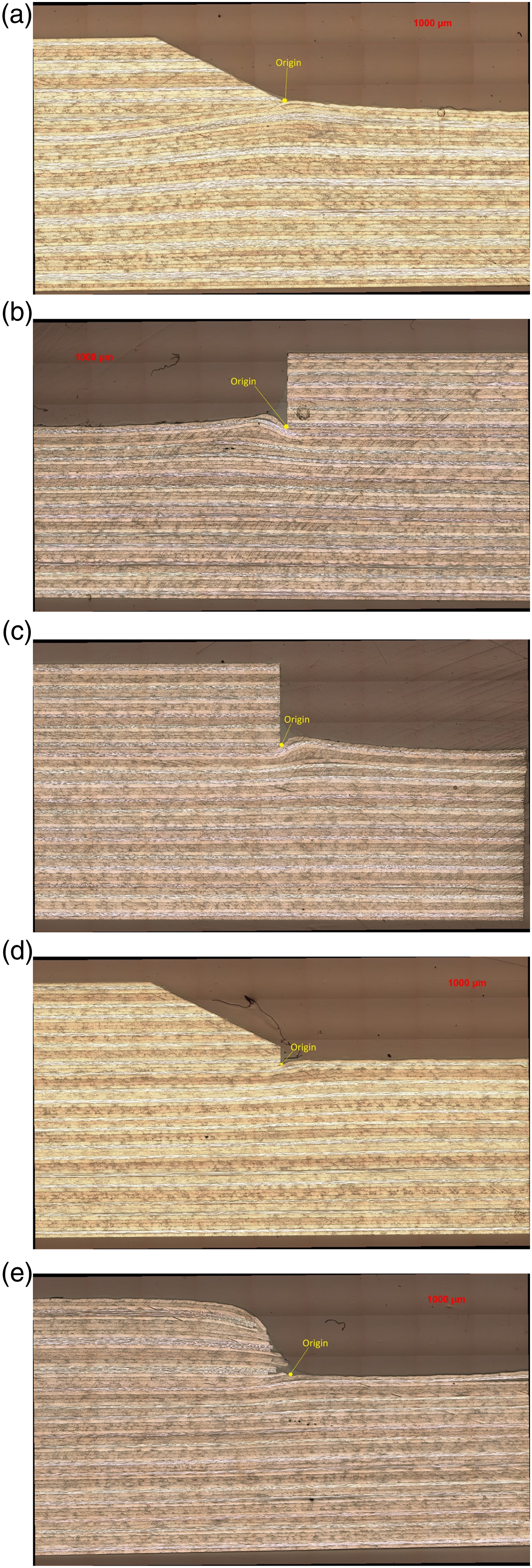

The original samples were two-part laminates, consisting of one full-length base laminate and a shorter upper block, as used in Ref.[⁷] A micrograph image was taken of each sample’s cross section view. These images were modified by covering the upper block in black colour using image editing software. The base laminate block was analysed and validated using the proposed algorithm in this paper. The stacking sequences of the samples are displayed in Table 1. The fibre direction was defined as 0° orientation in the horizontal direction and 90° into the plane. + and −45° orientations are grouped as one, referred to only as 45° ply, as they appear identical within the images. In the following sections, 0° ply, 45° ply, and 90° ply shall be referred to their respective fibre orientation direction. The nominal ply thickness of IM7-8552 and IMA-M21 were 0.125 mm and 0.165 mm, respectively. The readers are asked to report to the original study⁷ for more information on sample preparation as the focus of the present research is on automated micrograph analysis rather than defect formation in composites.

Table 1.

Laminate stacking sequence table.

Sample	Stacking sequence
IM7-8552 sample 1	[−45 90 45 0 0 45 90 –45]_3S
IM7-8552 sample 2	[−45 0 45 90 90 45 0 –45]_3S
IM7-8552 sample 3	[−45 0 45 90 90 45 0 –45]_3S
IM7-8552 sample 4	[−45 0 45 90 90 45 0 –45]_3S
IM7-8552 sample 5	[−45 0 45 90 90 45 0 –45]_3S
IMA-M21 sample 1	[−45 0 45 90 90 45 0 –45]_2S
IMA-M21 sample 2	[−45 0 45 90 90 45 0 –45]_2S
IMA-M21 sample 3	[-45 0 45 90 90 45 0 –45]_2S
IMA-M21 sample 4	[−45 0 45 90 90 45 0 –45]_2S
IMA-M21 sample 5	[−45 0 45 90 90 45 0 –45]_2S

Coloured optical micrograph images of the specimen edges were taken (with 0° fibres running along the horizontal direction and 90° fibres running perpendicularly to the plane of the images). The stacking sequence and its geometry were captured by the microscope with minimum distortion and high clarity. The samples were taken with an average 0.0145 mm/pixel resolution, allowing for sufficient microscale details from the studied samples to be captured. The images were subsequently pre-processed by the MATLAB code, which is described in the following sections, to aid the ply detection algorithm. All the steps in the algorithm were executed in MATLAB R2020b.

Image processing

The coloured image was first converted to a greyscale image using the inbuilt MATLAB ‘rbg2grey’ function. The brightness information of the pixels in the image remained. The pixel brightness value ranges from 0 (black) to 255 (white).

The image was further altered by the inbuilt 2D Gaussian filter, ‘imgaussfilt’ function in MATLAB. This process reduced the noise and smoothed the pixel brightness in the high resolution but noisy images. The 0° ply presented a large amount of noise within the ply. The cut was parallel to the fibre direction, and long strands of reflective (white) fibres could be seen sandwiched between dark resin. The Gaussian filter function filtered out most of the noise in the image. The 45° ply and 90° showed circular and elliptical fibre cross-sections, respectively, and displayed a more uniform pixel intensity. Finally, the image contrast was increased using inbuilt ‘imadjust’ MATLAB function. Figure 3 shows the image before and after processing.

Figure 3.

Pre-processed images. (a) Full length laminate section image, (b) Grey scale image and (c) Processed image.

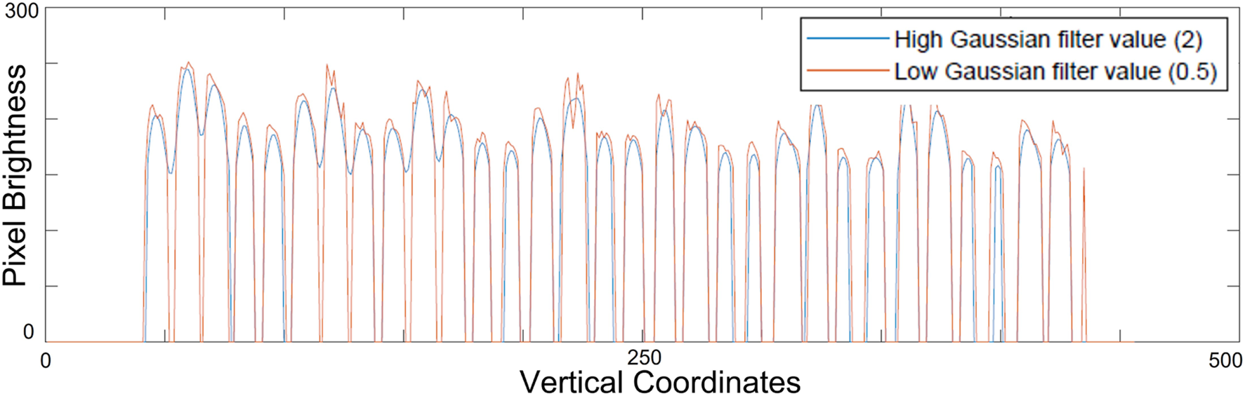
A preliminary study was carried out on the optimal Gaussian filter value by trial and error. The value of one was chosen to provide a balance between sufficient noise removal and preservation of the ply-matrix boundary, shown in the Figure 6 below. This value was more universal and worked well with most of the images. It was, however, highly dependent on the image quality and the type of composite laminates used. For IMA-M21 variants, a higher filter value such as two could be used because there was a significant brightness difference between ply boundaries. As for IM7-8552 variants, a value higher than 1 may risk removing fine details of the ply boundaries that separate the different plies in the image. The Gaussian filter is a balance between clarity of image and number of points detected described in the following section. A low filter value may lead to the results from the algorithm below becoming unstable.

Figures 4 and 5 illustrate the slice of image used in the Figure 6 demonstration. ‘w’ was the width of the image slice discussed in the following section.

Figure 4.

Illustration of one slice of the whole image, displayed by the yellow box.

Figure 5.

Image of one slice image shown in Figure 4 to be processed by the algorithm.

Figure 6.

Result difference of high and low Gaussian filter value of the image slice in Figure 5.

The ply-book knowledge was used to aid the identification of the ply coordinates. It contained the ply stacking sequence and the length of each ply in the sample. The ply length was not utilised at the moment in this algorithm presented but it would be included for the future which aimed to analyse tapered laminates that contained different ply lengths.

Point detection

The image pixel brightness value was used to determine the possible locations of the ply centre lines. The image can be represented in a matrix of pixel brightness values with columns (j) and rows (i).

First, the image is split into a series of image slices, each with an equal horizontal distance (d). The distance value is dictated by the horizontal distance between each planned finite element node in the final mesh. Every image slice was assigned its own slice ID, in ascending order from left to right of the image. A larger slice spacing resulted in quicker execution speed as fewer points were required to analyse, but sacrificed accuracy as it was also more likely to miss out minor details and waviness. The slice spacing can be determined by users for the level of detail required. A value of five pixels was used in this paper.

While the algorithm split the whole image into a series of small vertical slices of images, the width of each slice was determined by an image slice width value (w). This value was used to average the image horizontal brightness values of the pixels within each slice using equation (1).

{\bar{P}}_{i, j} = \frac{\sum_{i}^{i + w} P_{i, j}}{w}

(1)

where P_i,j and

{\bar{P}}_{i, j}

are the raw and averaged pixel brightness of the image, respectively.

The process averaged the overall pixel intensity of the ply by smoothing the dark and bright spots as shown in Figure 5. The process was done in the horizontal direction only to preserve the ply boundary contrast in the vertical direction. It is recommended that the image slice width value (w) is larger than the horizontal slide spacing (d). Each successive slice of an image would overlap each other and thus capturing the most details. The value of 10 pixels for the image slice width (w) was used in the paper. The node distance and image slice width were a balance between speed and level of details of geometry.

Pixels with brightness below the threshold of 150 were reduced to 0 brightness. This threshold was found by trial and error to be the best for use on IMA-M21 samples to sharpen the ply boundary. The difference in pixel brightness of the image in the vertical direction was exploited to identify the locations of each ply. A scatter diagram of the pixel brightness of each slice was produced and a spline was fitted to the data shown in Figure 7. The bright and dark pixels within each image slice formed peaks and troughs in the spline diagram. The coordinates of local maxima and points of inflection of the spline were recorded (using MATLAB findpeaks function) as the positions of the possible centre of the plies as shown as the orange points in Figure 7. The x coordinates of the scatter diagram form the vertical coordinate of the final geometric model while the horizontal geometric coordinate was denoted by the slice spacing (d). These points were saved as the column of a matrix for each slice. To complete the finite element model, each ply node would need to be assigned to a specific element and connected together. Another strategy would consist in identifying ply boundaries instead of their centres. However, this was trialled and shown to be less robust for micrographs of poorer quality and where the interfaces are not as well contrasted from the plies as in IMA-M21.

Figure 7.

Detected locations of possible coordinated of ply in an image slice.

As the resolution increases, the noise, specifically in 0° ply, created multiple peaks within short intervals as the peaks corresponded to the white spots in the image. For some images, most notably IM7-8552 laminates, there was little brightness difference between each ply, especially if the plies were in the same orientation which had similar average intensity. The algorithm would not be able to pick up the individual coordinates effectively. These artifacts caused the algorithm to pick up more or fewer points than the total number of plies in that slice of image and would need to be corrected by lowering the Gaussian filter value in the section above and using the following sections of the algorithm.

Ply thickness determination

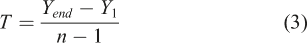
The ply thickness determination step determines the thickness of each ply in the laminate along the length and is used to influence the algorithm decisions in the following sections. This step was performed on every image slice along the length. It is because the laminate experienced major change in its thickness. The initial calculated thickness was not accurate to use for the whole image. A calculated thickness value can be calculated from the following equation (2). The ideal thickness was calculated using equation (3) by taking the first and last point identified by the algorithm using the equation. These two points were the top and bottom boundary of the laminate.

t = Y_{j - 1} - Y_{j}

(2)

where t is the distance between each point and Y is the vertical coordinate of the points.

T = \frac{Y_{e n d} - Y_{1}}{n - 1}

(3)

where T is the theoretical thickness of each ply, n is the number of plies in that particular slice.

A normal distribution of the thickness was analysed and produced a mean and standard deviation of the apparent ply centreline spacing. An ideal detection from the algorithm should produce a mean value close to the real thickness of the sample laminate and a small standard deviation. A histogram of the ply thickness was produced and compared to the normal bell curve as in Figure 8. The ideal histogram should fit within a normal bell curve and have a mode near the mean value with minimal outliers.

Figure 8.

Normal distribution and histogram of ply thickness in a single slice. (a) Raw detection and (b) After processing.

Identification of initial starting locations

However, it can be seen from Figure 8(a) that the obtained histogram for the ply thickness does not follow a normal distribution and seems to ‘merge’ two distinct normal distributions instead. To better identify the initial starting position of each ply and determine the correct average ply thickness (that will influence the decisions in the later steps on the algorithm), an extra processing step was added. A ply thickness check was conducted (on the distribution presented in Figure 8(a)) to measure the distance of each ply centreline from each other by comparing the coordinates using equation (2). The algorithm took the number of plies in the ply book and compared it to the number of peaks measured from the image. It then compared the ply thickness calculated from the equation (2) below and adjusted the initial starting positions to fit the average thickness closer to the mean value.

By comparing the thickness of each ply, the algorithm was able to detect if some ply separations were too large or small. The assumption was that the thickness of all the plies within the same slice should have minimal difference. This method heavily relied on the accuracy of the point detection algorithm in the above section. To aid the accuracy of laminate boundary detection, a manual coordinate identification method using the inbuilt MATLAB ‘ginput’ function was performed to mark the top and bottom coordinates directly from the image.

This minor manual step was especially important to help to remove incorrect detection of the background or the incomplete detection of the laminate boundary due to low resolution in the image. The last ply coordinate is incorrectly identified, shown in green in Figure 9. It should be emphasised that this step was only needed to be performed in the very first slice of each image since it was crucial to obtain accurate ply locations at this initial step. This manual step was not always required for images with high-quality resolution and contrast.

Figure 9.

Initial automatic point detection (blue and green points) and manual correction (red circles).

Once the ideal thickness was calculated, it was compared with the sample thickness calculated by the normal distribution from the identified ply points. The algorithm adjusted the points in the initial slice until the thickness fitted well with the bell curve as shown in Figure 8(b) and the number of measured points was equal to the number of plies. Each ply point was assigned a unique ply ID. This ID corresponded to the ply stacking sequence to which the following ply points belonging to this ply would be assigned. It also acted as the connectivity in the finite element model. This ID became the reference to determine the ownership of the unsorted ply points in the subsequent slices of images.

Connection of ply points in the image

After the whole image was analysed using methodologies described above and the average thickness of the whole laminate was calculated, the points were connected to form a continuous ply by the algorithm. The points attained the slice ID corresponding to their horizontal location. The points in each slice would be reorganised and assigned ownership to the corresponding ply ID in the following steps. The points identified were overlaid on the original sample image shown in Figure 10 below.

Figure 10.

Identified points of the whole image (IMA-M21 Sample 3).

Although the peak brightness points of the image were identified, they were not sorted and assigned to their ply ID. The task of connecting the ply points together in a single line for each ply first made use of a minimum difference technique. The algorithm iterated through each slice, from left to right, and through every ply in each image slice, from top to bottom.

The terminology ‘master’ and ‘slave’ referred to all aspects associated with the processed image slice and unprocessed slices, respectively. The method started by taking the coordinate of all the points in the master slice as a reference. For each master point, the closest corresponding slave point was determined from the following slave slice. Since the horizontal distance was fixed by the slice distance, only the vertical distance was analysed. The algorithm assumed that the composite laminate ply in the sample exhibited relatively small vertical deflection compared to the horizontal distance. This enabled the algorithm to only calculate the difference based on the vertical coordinates of the points. The slave point with the minimum distance to the master point was recorded and assigned to the same ply ID. This process was repeated for all the image slices.

Though effective, the technique assumed the ideal situation where the number of points identified in each slice was the same as the actual number of plies. This, however, was seldom true as the peak intensity algorithm would often detect fewer or more points depending on the quality of the image and the Gaussian blur value. The common artifacts from the algorithm were the missing points shown in green and the noise in the image causing additional peaks created shown in red in Figure 11.

Figure 11.

Identification of ply points in a noisy image (IM7-8552 Sample 1).

This process was therefore coupled with several additional decision algorithms described in the section below to determine the correct ply ownership of the slave points. Figure 12 illustrates that the same slave point would be owned by two different plies in some cases. The black crosses represented the ‘master’ slice points and the green as ‘slave’ points. The red point is grouped into two different ply groups because of its proximity to both ply points denoted by the blue and green arrows.

Figure 12.

Illustration of the situation when a single ‘slave’ point is identified to be in two different ply groups. (a) The point belongs to the ply on top and (b) The point belongs to the ply below.

A comparison of the distance was done between the two points and it was assigned to the closest ply point (shown as the green arrow) while the connectivity already assigned to the other ply ID (shown in blue arrow) was removed. An additional point distance check using equation (2) was carried out on the slave point to determine whether the distance of the slave point, compared to the point above, it fell within the thickness threshold calculated by equation (3) in each slice of the laminate. If the distance was too large or too small, the point was subsequently discarded.

The ply assignment step for all the 0° ply were skipped. The noise from 0° ply could easily cause the ply to be assigned an incorrect location when comparing the minimum distance of the master and slave ply points. The 0° ply point was therefore initially not assigned to have any subsequent point. This enabled the surrounding plies to enforce a boundary around the 0° plies as they acquired their respective points. The empty points of the 0° ply were automatically created by the algorithm.

The algorithm always takes the first detected point as the top ply point. This assumed that it has a clear laminate boundary. The ply would follow closely to the actual laminate boundary which was important as it was the outermost ply. If the detected ply point was already selected for the previous ply, the algorithm compared its relative distance to their respective master point and decide which ply the double detected point belonged to.

Once all the image slices were processed, the algorithm followed up to fill in the remaining empty points using the equation (4) below. An equal distance method was used to approximate the possible locations of the missing ply points. The boundaries in the calculations were the known points already identified in the slice. By dividing the distance between the two boundary points into equal distance intermediate points, the empty points were filled with coordinates on which a ply may lie on.

Y_{j} = \frac{Y_{n} - Y_{m}}{n - m} + Y_{j - m}

(4)

where n and m are the indexes of the closest non-empty points before and after the current point.

This method did not make use of the existing knowledge of the points identified in the peak point algorithm. However, it provided a simple and quick solution that could present intermediate solutions to be used as a reference master point for the algorithm in the next slice. The assumption that the plies shall have an equal thickness in the missing points were valid as the laminate should be packed and compressed tightly by the high pressure in the curing process.

A common error introduced by this technique was ply drift, which is most prominent in images with very high amount of noise. As seen in the Figure 11 circled in red, the peak intensity points in the 0 ply did not necessarily lie in the middle of the ply, and would sometimes have two or more peaks within the same ply. The algorithm would mistakenly take one of the misaligned points as a ply point, with the error then propagating downwards with more errors. This phenomenon is explained in more detail in the following section. By removing the slave point errors in the algorithm and estimating the empty points based on the boundary plies identified from more accurate image data, the total accuracy of the whole algorithm and the ply points is increased. This technique removed the possibility that an incorrectly identified ply point within the 0° ply propagates the error into the following slices.

In the cases that the top or bottom ply does not have identified points, as displayed in Figure 13, artificial centre-line ply points were added to the ply by duplicating the closest slave point and shifting it to the outside of the laminate by the distance of one ply thickness. This method is only used if there is no information captured on the boundary plies from the image and thus the node must be artificially created.

Figure 13.

Illustration of empty ply point on the top ply (IMA-M21 Sample 3).

A final thickness check was conducted at the end of the process in each slice. The algorithm calculated the distance between all points within the slave slice and compared them to the reference thickness in the master slice. The point coordinates were altered if the distance falls beyond the thickness threshold. The thickness threshold was taken to be 1.5x the mean ply thickness as shown in Figure 8 by trial and error.

Decision tree

The full algorithm and its decision tree is displayed in Figures 14 and 15. Each ply point was processed by the decision algorithm. This algorithm determined whether the selected point in the image slice is the correct location for the ply. If the point is determined to be incorrect, the algorithm removed the point from the ply and left it to be filled in the later stage as stated in the above section.

Figure 14.

Algorithm flow diagram.

Figure 15.

Algorithm decision diagram.

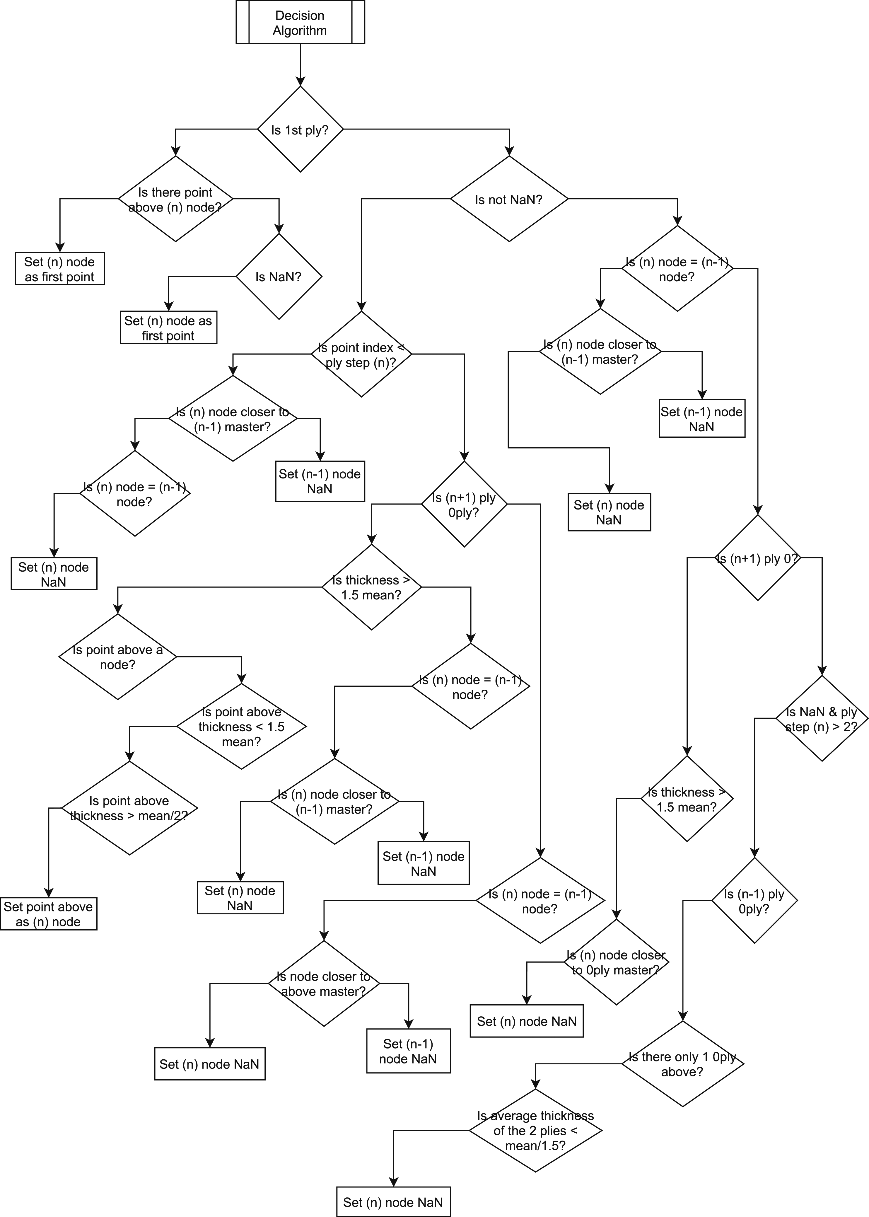
Where the decision point ends, the algorithm exits the branch and continues to the next step. ‘Master’ means previously determined ply point. (n) is the current ply, (n − 1) is the ply above, (n + 1) is the ply below.

Smoothing Ply centre lines

Figure 16 shows the assignment of the ply points to their ply ownership. Some artifacts could be introduced to the final laminate geometry by the discussed algorithm above which can be observed in Figure 17. These artifacts caused the ply lines to have sharp and irregular spikes due to mapping and detection errors. A smoothing algorithm was employed to remove the irregular spikes and create a continuous spline using the inbuilt MATLAB ‘smoothdata’ function and moving mean method. A value of five for the algorithm was chosen from trial and error to remove unwanted spikes while preserving most of the minor true waviness of the sample shown in Figure 18.

Figure 16.

Assignment of points to the designated ply groups. (IMA-M21 Sample 3) (a) Before assignment, (b) After assignment.

Figure 17.

Zoomed in comparison of before and after smoothing ply centreline points. (IMA-M21 Sample 3) (a) Before smoothing, (b) After smoothing.

Figure 18.

Smoothed ply centreline points (IMA-M21 Sample 3).

Finite element mesh generation

The result from the algorithm is the coordinates of the central line of each individual ply. A finite element model requires the boundary coordinates of each ply. Each ply model had to be created separately. The geometry of each ply followed their ply points as the centre-line. The boundary nodes of each ply were created by building a node in the middle of two adjacent plies. Each ply shared the same boundary if they were in contact with each other as shown in Figures 19 and 20.

Figure 19.

IM7-8552 Laminate ply finite element boundaries. (a) IM7-8552 Sample 1, (b) IM7-8552 Sample 2, (c) IM7-8552 Sample 3, (d) IM7-8552 Sample 4 and (e) IM7-8552 Sample 5.

Figure 20.

IMA-M21 Laminate ply finite element boundaries. (a) IMA-M21 Sample 1, (b) IMA-M21 Sample 2, (c) IMA-M21 Sample 3, (d) IMA-M21 Sample 4 and (e) IMA-M21 Sample 5.

As illustrated in Figures 21 and 22, the software then created 3D hexahedral elements of the laminate and wrote them into an input file for the FE package Abaqus. Each node was projected in the direction perpendicular to the micrographs’ plane and 3D bricks were created by linking facing planes at the top and bottom of the ply, respectively.

Figure 21.

IM7-8552 Laminate finite element models. (a) IM7-8552 Sample 1, (b) IM7-8552 Sample 2, (c) IM7-8552 Sample 3, (d) IM7-8552 Sample 4 and (e) IM7-8552 Sample 5.

Figure 22.

IMA-M21 Laminate finite element models. (a) IMA-M21 Sample 1, (b) IMA-M21 Sample 2, (c) IMA-M21 Sample 3, (d) IMA-M21 Sample 4 and (e) IMA-M21 Sample 5.

Results analysis

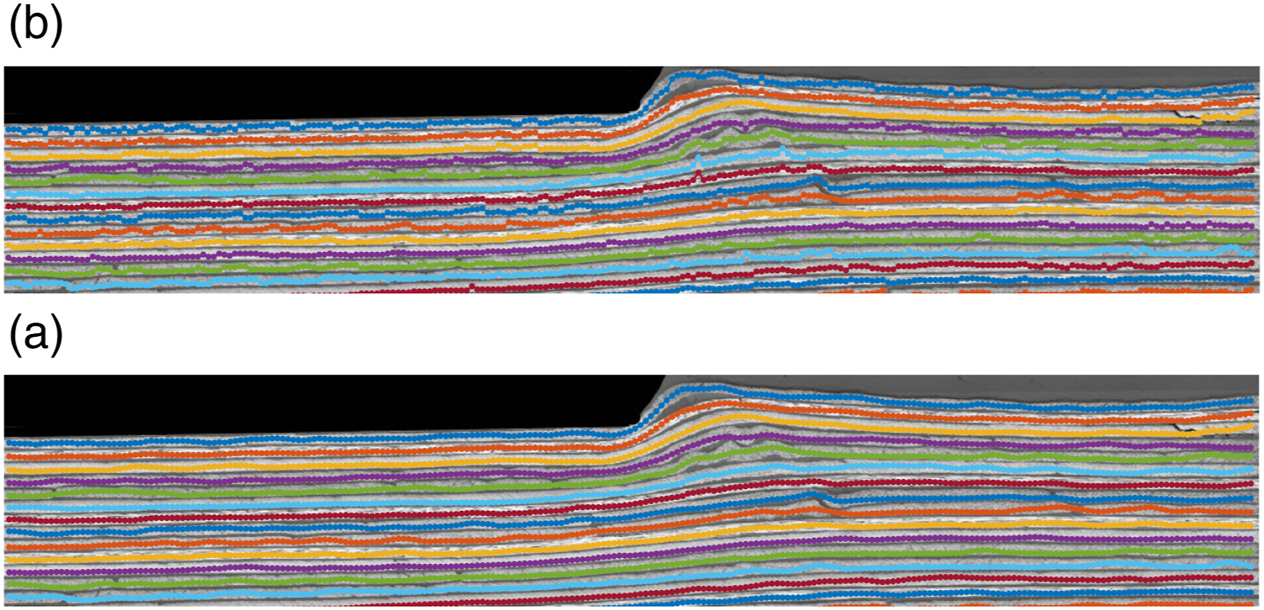
The proposed methodology was validated qualitatively by visual inspection. The assessment was completed by superimposing the finite element nodes onto the sample images as illustrated in Figures 23 and 24. The images were analysed and the geometries were compared against the real laminate. All results were created fully automatically, using the settings shown in Table 2 and without any user interaction.

Figure 23.

IM7-8552 Laminate finite element boundaries overlaid on the original sample image. (a) IM7-8552 Sample 1, (b) IM7-8552 Sample 2, (c) IM7-8552 Sample 3, (d) IM7-8552 Sample 4 and (e) IM7-8552 Sample 5.

Figure 24.

IMA-M21 Laminate finite element boundaries overlaid on the original sample image. (a) IMA-M21 Sample 1, (b) IMA-M21 Sample 2, (c) IMA-M21 Sample 3, (d) IMA-M21 Sample 4 and (e) IMA-M21 Sample 5.

Table 2.

Laminate stacking sequence table.

Setting	Values
Pixel brightness threshold	150
Image slice width (w)	10 pixels
Node distance (d)	5 pixels
‘Imgaussfilt’ setting	1
‘Imadjust’ setting	‘Stretchlim’
‘Smoothdata’ setting	‘Movemean’, 5

The ‘as-manufactured’ geometries matched well with the sample images, able to capture the change of shape in the middle of the sample. The algorithm was able to filter out the scratches on the laminate cross-section. The only difference was the absence of the ply gaps in the compression region due to a single boundary between two plies.

The algorithm was able to capture the small waviness of ply 4–9 due to compression in IMA-M21 Sample 3 as shown in Figure 25 in yellow. The algorithm was also able to create a relatively good representative model for IM7-8552 samples. However, due to the high amount of noise in the image, the result presented small deviations from the real geometry.

Figure 25.

Illustration of high accuracy result of IMA-M21 Sample 3 from the algorithm. (a) IMA-M21 Sample 3 boundary lines overlaid on the sample image, (b) Zoomed in view of (a) on the yellow box.

Algorithm execution time

The goal of the proposed algorithm was to reduce the time needed to create ‘as-manufactured’ finite element models of real composite laminate samples. The execution time of the algorithm on the various samples was recorded in Table 3.

Table 3.

Algorithm execution time for the various samples.

Sample	Execution time (seconds)
IM7-8552 sample 1	21
IM7-8552 sample 2	23
IM7-8552 sample 3	22
IM7-8552 sample 4	22
IM7-8552 sample 5	23
IMA-M21 sample 1	17
IMA-M21 sample 2	18
IMA-M21 sample 3	18
IMA-M21 sample 4	16
IMA-M21 sample 5	21

As seen from Table 3, the time to create a full ‘as-manufactured’ finite element model from an image took from 15 to 30 s. This was significantly shorter than creating the finite element model manually which can take between half an hour and several hours of work.

Conclusions

A novel methodology to identify and create the ‘as-manufactured’ geometry of individual plies from a 2D image of a composite laminate specimen has been presented. The methodology incorporated image processing techniques and a novel 2D point mapping and smoothing algorithm. The proposed algorithm could be applied to most 2D scans of composite laminates with various degree of waviness in a fast and automated manner with none to minimal user interaction. Furthermore, only a relatively low image resolution was needed which saved scanning time and storage requirement and allowed for lower resolution microscopic imaging equipment.

The algorithm was able to capture the ‘as-manufactured’ geometry of the ply curvature which differed from the ‘as-designed’ geometry. The ply points were assigned to their ID and their information could be extracted and modified individually without affecting other points in the data structures.

The geometrical information of the identified plies could be used for various purposes. First, using further in-house code the composite laminate geometry could be converted into a 3D finite element mesh for stress and strength simulations. The user has the flexibility to adjust the final model resolution and refinement level. Second, the geometry created by the algorithm captures the deformation of each ply in the laminate sample. One can study the ‘as-manufactured’ geometry deviation of the sample from the ‘as designed’ model after the manufacturing, providing better insight into the phenomena happening during the fibre and ply compression. By doing so, a better understanding of composite structure manufacturing effects can be obtained, which can aid the design of complex composite structures with minimal defects. Currently, the algorithm can only deal with plies of the same length and this is an obvious improvement that needs to be done in the future. Although the tool presented here only works for laminates with continuous plies, it sets the basis for a more general tool that could deal with more complex composite designs such as tapered laminates with ply terminations (see Figure 26).

Figure 26.

Tapered composite laminate sample.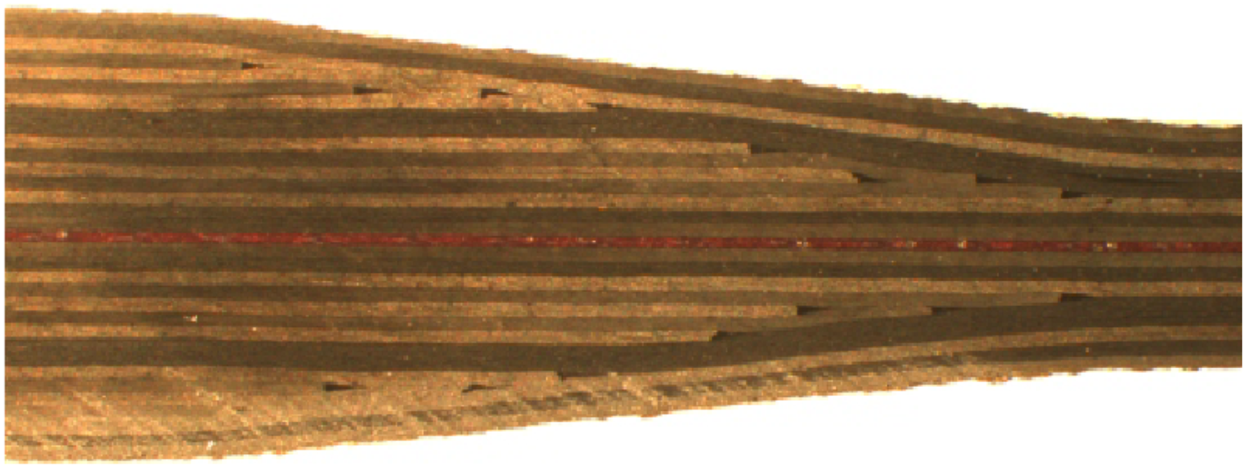

Footnotes

Acknowledgements

The authors would like to thank Dr James Kratz (University of Bristol) for providing the micrographs used in this study. The work was funded by the Engineering and Physical Sciences Research Council (EPSRC) through the platform grant ‘Simulation of new manufacturing Processes for Composite Structures (SIMPROCS)’ (grant no. EP/P027350/1). The code dteailed in the manuscript is distributed for free from the Bristol Composites Institute Github page () and access can be requested by e-mailing bcigithub@bristol.ac.uk.

Declaration of conflicting interests

The author(s) declared no potential conflicts of interest with respect to the research, authorship, and/or publication of this article.

Funding

The author(s) disclosed receipt of the following financial support for the research, authorship, and/or publication of this article: This work was supported by the Engineering and Physical Sciences Research Council (EP/ P027350/1).

ORCID iDs

Pok Lam Marvin Lau

Jonathan P-H Belnoue

Stephen R Hallett

References

Rawal

Misra

Wendt

. Composite materials for space applications. NASA Contractor Report 187472, 1990.

Hull

Clyne

. An Introduction to Composite Materials. Cambridge Solid State Science Series). 2nd ed.. Cambridge: Cambridge University Press, 1996, https://doi.org/10.1017/CBO9781139170130

Toubal

Karama

Lorrain

. Stress concentration in a circular hole in composite plate. Composite Structures 2005; 68: 31–36, https://doi.org/10.1016/j.compstruct.2004.02.016

Hoa

Ganesan

. The study of tapered laminated composite structures: a review. Compos Science and Technology 2000; 602643–2657, https://doi.org/10.1016/S0266-3538(00)00138-X

Muc

Ulatowska

. Local fibre reinforcement of holes in composite multilayered plates. Composite Structures 2012; 94(4): 1413–1419, https://doi.org/10.1016/j.compstruct.2011.11.017

Zhang

Kawashita

Jones

Lander

Hallett

. An experimental and numerical investigation into damage mechanisms in tapered laminates under tensile loading. Composites Part A; 133(2020): 105862, https://doi.org/10.1016/j.compositesa.2020.105862

Varkonyi

Belnoue

JPH

Kratz

Hallett

. Predicting consolidation-induced wrinkles and their effects on composites structural performance. Int J Mater Form; 13(2020): 907–921, https://doi.org/10.1007/s12289-019-01514-2

Abdulhamid

Bouvet

Michel

Aboissière

Minot

. Influence of internally dropped-off plies on the impact damage of asymmetrically tapered laminated CFRP. Compos. Part A 2015; 68: 110–120, https://doi.org/10.1016/j.compositesa.2014.09.024

Dilonardo

Nacucchi

De Pascalis

Zarrelli

Giannini

. High resolution X-ray computed tomography: A versatile non-destructive tool to characterize CFRP-based aircraft composite elements. Composites Science and Technology 192; 2020: 108093, https://doi.org/10.1016/j.compscitech.2020.108093

10.

Naouar

Vidal-Salle

Schneider

Maire

Boisse

. 3D composite reinforcement meso F.E. analyses based on X-ray computed tomography. Composite Structures 2015; 132: 1094–1104, https://doi.org/10.1016/j.compstruct.2015.07.005

11.

Naouar

Vidal-Salle

Schneider

Maire

Boisse

. Meso-scale FE analyses of textile composite reinforcement deformation based on X-ray computed tomography. Composite Structures 2014; 116: 165–176, https://doi.org/10.1016/j.compstruct.2014.04.026

12.

Nikishkov

Makeev

. Finite element mesh generation for composites with ply waviness based on X-ray computed tomography. Advances in Engineering Software 2013; 58: 35–44, https://doi.org/10.1016/j.advengsoft.2013.01.002

13.

Czabaj

Riccio

Whitacre

. Numerical reconstruction of graphite/epoxy composite microstructure based on sub-micron resolution X-ray computed tomography. Composites Science and Technology 2014; 105: 174–182, https://doi.org/10.1016/j.compscitech.2014.10.017

14.

Potter

Pinho

Robinson

Iannucci

McMillan

. Mesh generation and geometrical modelling of 3D woven composites with variable tow cross-sections. Computational Materials Science 2012; 51(1): 103–111, https://doi.org/10.1016/j.commatsci.2011.06.034

15.

Wijaya

Ali

Umer

Khan

Kelly

Bickerton

. An automatic methodology to CT-scans of 2D woven textile fabrics to structured finite element and voxel meshes. Composites Part A 2019; 125105561, https://doi.org/10.1016/j.compositesa.2019.105561

16.