Sage Journals: Discover world-class research

Abstract

A common braiding machine cannot perform continuous braiding using closed annular axis mandrels. To solve this problem, a modified vertical braiding machine was made to braid composite preforms with irregular cross-section mandrels. The finite element method was used to simulate the braiding process, and an efficient method was also derived to predict the braiding angles. The results show that the predicted braiding angles are basically consistent with the actual braiding angles, and the braiding angles at distinctive locations on the braided preform recorded differences of up to 10° or more than 30%. Braiding process simulation via the finite element method can thus effectively and vividly reflect the yarn path on the preform. As such, the braiding angles on the braided preforms can be realized through projection and surface flattening with much better accuracy. It also resolves the difficult problem often faced in measuring the braiding angles at the corner of the mandrel and provides a solid basis for continued research on the performance of its composite reinforcement.

Keywords

braiding mandrel braiding angle FEM simulation

Introduction

Industrial braiding machine is usually divided into vertical braiding machine and horizontal braiding machine, working on the principle where multiple driving plates move two groups of yarn carriers in opposite directions to crisscross repeatedly and the carriers allow the yarn to cross-braid on the mandrel to form the braided preform.¹ One end of the yarn is driven by the carrier on the track board and the other end is fixed on the mandrel through the braiding ring.² The mandrel is usually linear and moves in a straight line³ under the traction of the driving device.⁴

In recent years, some researchers have studied the braiding process through finite element simulation. Pickett et al. used the PAM-Solid software to simulate the two-dimensional braiding process and compared the traditional analytical method with the finite element method.⁵ Hans et al. combined Matlab, Abaqus, and VB to study the braiding process of mandrels in different shapes.⁶ Swery et al. studied a complete simulation method during the processing of braided composite part.⁷ Wu et al. studied the numerical prediction method during the circular braiding process.⁸ All these researches showed that the finite element method was effective for simulation of the braiding process. However, the research objects were mainly limited to linear mandrels that have rather regular cross sections. The study on the braiding process of irregular cross-section mandrels, especially closed annular axis mandrels, is solely needed.

The braiding angle indicates the angle between the yarn and the axial direction of the mandrel.⁹ Braiding angle is the main technical parameter^10
–12 to represent the braided preform and it shows the yarn direction and determines the structure of the braided preform,^13,14 thus influencing the mechanical property of the braiding composite reinforcement.^15,16 In terms of the standard linear cylindrical mandrel, the yarn’s braiding angles at different locations on the surface of the mandrel are theoretically the same and correspond to the radius of the mandrel, the carrier speed, and the mandrel’s take-up speed as shown in equation (1).^17,18 Therefore, the braiding angle of the linear cylindrical mandrel is a constant.^19,20

α = {tan}^{- 1} \frac{r \cdot ω}{v}

where α is the braiding angle, r is the radius of the mandrel’s cross section, ω is the angular velocity of the carrier, and v is the take-up speed of the mandrel.

As for the irregular cross-section mandrel, different radiuses at different locations of the mandrel lead to distinctive braiding angles at different mandrel’s locations and also a failure to express the equation through a constant. Especially so for annular axis braiding, the mandrel’s changing axial direction causes different braiding angles and difficulty in measurement. If fluctuation of the yarn’s tension and changes in the convergence area of the braiding yarns are taken into account, the braiding angles will be even more difficult to measure.

This article proposed a braiding method using a closed annular axis mandrel, which can be implemented after the finite element simulation of the braiding process is done and a method was effectively derived to predict the braiding angles at different mandrel’s locations. Since the braiding process’ simulation via the finite element method is capable of reflecting the yarn path on the braided preform more vividly, accurately, and easily, this provides a solid basis for subsequent research on the performance of its composite reinforcement such as bicycle rims.

Annular axis braiding

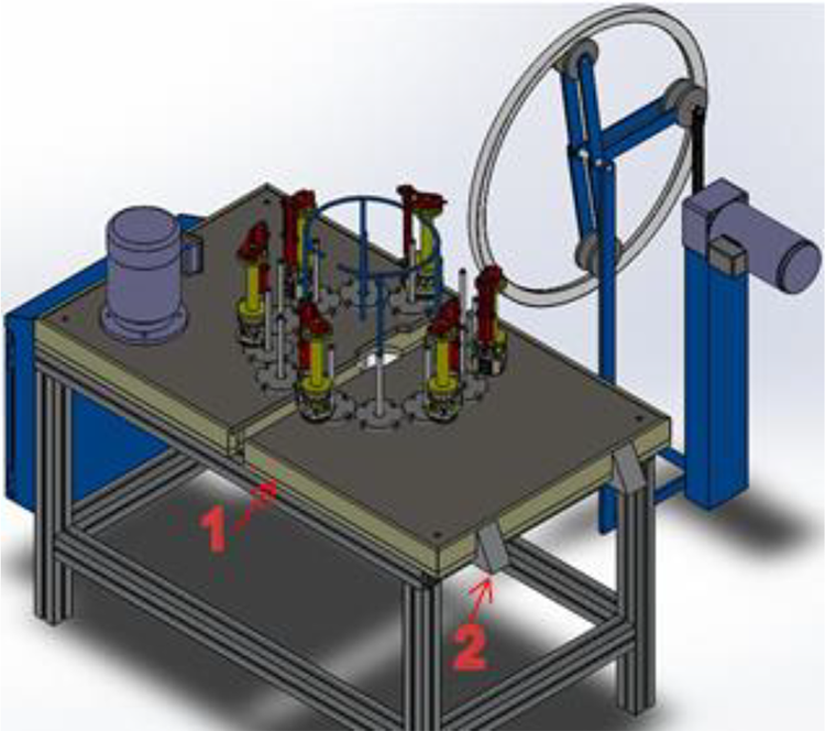
A common braiding machine cannot do direct braiding using a closed annular axis mandrel. A modified 12-carrier vertical braiding machine was applied in the braiding process, as shown in Figure 1. Different from a common braiding machine, the track board of the modified braiding machine could be opened and closed, which guaranteed free access to the closed annular axis mandrel in the braiding areas of the machine. Meanwhile, a set of annular axis mandrel driving device was applied to transfer the rotation of the roller to the annular axis mandrel, which allowed the mandrel to rotate around its center and achieve the annular axis braiding process. Besides, by adding a braiding ring that could be opened and closed, the mandrel driving device can pull the mandrel to move beneath the track board, instead of pulling the mandrel to move above the track board as the common braiding machine does. Under such conditions, the yarn’s convergence area was guaranteed to be perpendicular to the track board and located on the same horizontal line with the center of the mandrel. Then, the issue of the limited diameter of the track board of the braiding machine and the spatial restriction due to the limited diameter of the annular axis mandrel was solved.

Figure 1.

Schematic diagram of annular axis braiding machine (1: track board, 2: mandrel, 3: braiding ring).

The track board that can be opened and closed includes a fixed board, a movable board, a guide rail, and a stopblock. During fixing or removal of the mandrel, the movable board is pulled outward along the guide rail to the stopblock. After the mandrel is fixed or removed, the movable board is pushed back to its original position along the guide rail to connect to the fixed board. The braiding ring that can be opened and closed is supported by a braiding ring bracket. This bracket is divided into two parts. One part is installed on the fixed track board, and the other part is installed on the movable board, which can move synchronously with the movable board. When the track board is closed, the braiding ring is also connected as a whole. The schematic diagram of the movable board when it is opened is shown in Figure 2.

Figure 2.

Schematic diagram of open movable board of annular axis braiding machine (1: movable board, 2: stopblock).

Before commencing the braiding operation, the annular axis mandrel is sheathed on the mandrel’s driving device, and the movable plate is pushed outward along the guide rail to the stopblock, to separate from the fixed plate. Meanwhile, the braiding ring is also opened. Next, the mandrel’s driving device moves to push the mandrel into the convergence area at the center gap of the braiding machine’s track plate, and the movable plate is pushed back to the original position along the guide rail to connect with the fixed plate, to form a whole. The braided yarn is drawn out from the yarn carrier. The yarn passes through the braiding ring from the outside to the top and then moves downward, concentrating toward the mandrel’s direction. The yarn is bound to the surface of the mandrel and starts braiding. The braided preform is drawn by the mandrel driving device toward the bottom of the track board, as shown in Figure 3.

Figure 3.

Braiding machine using annular axis mandrel.

Once the braiding process is finished, the movable plate repeats the above action to separate from the fixed plate, and the braided preform and mandrel are taken out from the mandrel’s driving device. The actual braided preform is shown in Figure 4.

Figure 4.

Actual braided preform.

The material used for the mandrel is polypropylene. The mandrel is not removed immediately after braiding, but after the resin is cured to the preform. Holes need to be drilled on the material after resin curing, and the melting point of the mandrel material is not high, so the mandrel will melt and flow out of the holes at high temperatures. After the mandrel is removed, the annular axis braided composite with a similar shape to the closed ring mandrel can be obtained.

Simulation of braiding process

Considering the annular axis braiding, especially when the irregular cross-section mandrel is applied, the application of the finite element method for braiding process simulation enables effective and vivid reflection of the yarn path on the braided preform.^5

–8 Abaqus finite element software was used to simulate the annular axis braiding process with the assumption that the braiding yarn would be fixed on the mandrel and the friction between the yarns and the braiding ring was excluded from consideration.

The cross section of the mandrel applied in the braiding process was not of circular or any other regular shapes but of irregular shapes combining curves and a straight line as shown in Figure 5(a). Furthermore, the angle between the curves and the straight line was big and so was the angle at the bottom of the curves. It could be predicted that the yarns would turn sharply at the three corners. The complete structural model of the annular axis mandrel is shown in Figure 5(b). The radius of the closed annular axis mandrel is 255 mm.

Figure 5.

Annular axis mandrel model. (a) Cross section of the mandrel and (b) Mandrel model.

The finite element simulation model was constructed based on the real conditions. The model was made of braiding yarns, a braiding ring, and an annular axis mandrel as shown in Figure 6. The spring was used to connect the braiding yarns in the finite element model, so that the braiding yarns could maintain tension, just as the carriers would provide tension to the braiding yarns during actual braiding.

Figure 6.

Schematic diagram of finite element model of annular axis braiding.

The braiding yarn model was the key part in the simulation and required certain flexibility as well as good tensile strength. Therefore, a proper element type was needed.⁸ The truss element is connected by friction-free and freely rotatable hinges, usually divided into smaller and more numerous sections. Hence this article applied the truss element to construct the braiding yarn model. Each braiding yarn was divided into 300 truss elements to keep the yarn model with the flexibility of real braiding yarns. The mandrel and the braiding ring would not deform theoretically, so they were set as discrete rigid elements. The application of discrete rigid elements could reduce the calculating amount.⁵ A cut-section view of various elements in finite element simulation is shown in Figure 7.

Figure 7.

Cut view of various elements in finite element simulation (1: spring, 2: yarn, 3: braiding ring, 4: mandrel).

The braiding yarn setting in the simulation was the same with that in the braiding process, which was T700-12K carbon fiber with an elasticity modulus of 230 GPa²¹ and a density of 1800 kg/m³. The braiding craft in the finite element simulation is consistent with the craft used in the actual braiding process. Reasonable simulation model boundary conditions were set. The braiding ring was fixed and the mandrel rotated in the same velocity with actual state. Two groups of yarn carriers drove two groups of yarns to rotate in different directions according to the same angular velocity with actual state. Spring stiffness is set to 5E+07. The friction formulation between the yarn and the braiding ring is assumed to be frictionless, and the friction formulation between the yarn and the mandrel is rough.

The explicit dynamics model was selected to handle the large geometric deformation and complex contact issues. The explicit central difference algorithm was pretty suitable for the research on such nonlinear, large deformation braiding yarns’ materials. The penalty contact method was applied for the mechanical constraint formulation. It was required to avoid possible penetrative actions. As a result, a larger penalty stiffness value was preferred to generate a large contact force and avoid further contact penetration. The results after the simulation are shown in Figure 8.

Figure 8.

Simulation result of annular axis braiding process.

It can be seen from Figure 8 that both groups of yarns were interlaced and attached to the surface of the mandrel. Through the finite element method to simulate the braiding process, the yarn path can be accurately obtained, and the simulation results matched the actual braided preform to a high degree.

Post-processing method for measuring braiding angles

The yarn’s paths on the braided preform could be obtained through the finite element simulation of the annular axis braiding process. The simulation results reflected the view of the model in three-dimensional space and the yarn’s paths at different locations on the mandrel could be easily observed by rotating, zooming, or other methods. Nevertheless, since the mandrel and yarn’s paths were three-dimensional rather than two-dimensional, it was difficult to conveniently and accurately find out the front views of two yarns interlacing on the surface of the mandrel or measure the braiding angles one by one by rotating the three-dimensional model. The yarn path and the braiding angles of the three-dimensional braided preform cannot be visualized in two-dimensional form vividly. But the prediction method would help to efficiently measure the braiding angles at different locations on the mandrel in the simulation results. The specific prediction method is as follows.

Firstly, import the three-dimensional mandrel model to Solidworks or other three-dimensional modeling software in igs document format. The model in the three-dimensional modeling software should be consistent with the model in the Abaqus finite element simulation software, including the same coordinates. Take the quarter section as the research object and cut off the rest, as shown in Figure 9(a).

Figure 9.

The mandrel and yarn path reconstructed in Solidworks. (a) Quarter section of the mandrel and (b) imported yarn path.

In the Abaqus post-processing module, regenerate a deformed yarn path to form a new part. View the inp document in text format and the three-dimensional coordinates of all nodes on the yarn can be found. However, the three-dimensional coordinate data in the inp document require necessary conversion to a data format that can be directly imported into the three-dimensional modeling software. The editing in Excel software for data imported in txt format is used. Import the text document as the curve document and rebuild a new curve by entering the coordinate data as shown in Figure 9(b) in the three-dimensional modeling software including the quarter section of the mandrel. As a result, the deformed yarn path is rebuilt in the three-dimensional modeling software.

Then, the yarn path is required to be projected onto the surface of the mandrel. The projection tool in SolidWorks obtains the projection point on a target surface, by drawing a normal line from the point to the target surface. The intersection of the normal line and the target surface is the projection point. Select a node on the yarn, utilize the projection in the modeling software, and select the surface of the corresponding nodes on the mandrel to realize the normal projection point of the yarn’s node on the surface of the mandrel as shown in Figure 10(a). Project all nodes on the yarn onto the corresponding mandrel surface and construct the curve through XYZ points to connect all projected points from one end of the yarn in an orderly manner. As a result, the projection curve of the yarn path on the surface of the mandrel is realized as shown in Figure 10(b). Since the projection point is very close to the original point, the projection curve on the mandrel surface is also very close to the original yarn path. The only difference is that the original yarn path undulates on the surface of the mandrel, whereas the projection curve is entirely on the mandrel surface. Therefore, for the measurement of braiding angles and yarn spacing, the projection method has little effect on the accuracy of these measurements.

Figure 10.

Yarn node point and yarn path projected on the mandrel surface. (a) Node point projected on mandrel surface and (b) yarn path connecting projection points.

Next, the mandrel surface will be flattened. The whole annular axis mandrel cannot be flattened because it is three-dimensional and a closed ring of full circle. But for the quarter section of the mandrel, if it is cut along an edge, the mandrel surface can be flattened to a two-dimensional plane. In addition, since the flattened area is not too large, the influence of distortion during the flatten process is limited. Select the surface with yarn on the quarter section of the mandrel and flatten the mandrel surface alongside one edge of the surface. Meanwhile, the projection curve mentioned above should be flattened as well as shown in Figure 11.

Figure 11.

Flattening of mandrel surface.

The flattened quarter section of the mandrel is shown in Figure 12(a). The path in the plane is the projection curve of the yarn path on the mandrel surface. It can be seen that the yarn path turns sharply at the intersection of the plane and the curved mandrel surface, which is the same as the real braided preform. The same step is used to flatten other projection curves of the yarn path. Two groups of yarns with different rotating directions are distinguished by using different color marks. One projection curve of the yarn path is flattened at a time, and each flattened surface is saved as a part separately in the three-dimensional modeling software. And then all flattened surfaces are completely overlapped and displayed together in a new assembly document. Finally, all the projection curves of the yarn path flattening results can be obtained, as shown in Figure 12(b). The two vertical yellow lines on the flattened surface in Figure 12(b) are the two sidelines on the outside of the mandrel.

Figure 12.

Flattened mandrel surface with yarn path. (a) Flattened surface with yarn path and (b) overlapping surfaces with all yarns.

With all yarns flattened on the mandrel surface, the angles between two yarns on the braided preform can be vividly displayed and the angles can be easily measured by image processing software. The measurement tool in Image-Pro Plus software facilitates the measurement of angles between yarns as shown in Figure 13. Set appropriate features, measurements, labels color, and line width in display colors and settings options for better display of the angles and more accurate measurement results.

Figure 13.

Measuring braiding angles.

Results

According to the braiding angles’ prediction method, the average value of braiding angles is 35.6°, the maximum value is 48.5°, the minimum value is 27.1°, and the standard deviation is 5.29, as shown in Table 1. If the mandrel surface is divided into three sectors by two sidelines on the mandrel’s outer sections, the average values of braiding angles in the three sectors are 34.0°, 39.6°, and 34.0°, respectively.

Table 1.

Statistical results of braiding angles.

Braiding angles	Sector 1 average	Sector 2 average	Sector 3 average	Overall average	Maximum value	Minimum value	Standard deviation
Predicted	34.0	39.6	34.0	35.6	48.5	27.1	5.29
Actual	34.8	37.8	36.6	36.2	43.9	28.0	3.28

The reliability of the prediction method could be verified by measuring the actual braiding angles on the surface of the real braided preform. Take photos of the three surfaces of the real braided preform, respectively, corresponding to the three sectors of the mandrel surface mentioned above, and use the image processing software to measure the braiding angles of the three sectors, as shown in Figure 14.

Figure 14.

Measurement of actual braiding angles. (a) Sector 1, (b) sector 2, and (c) sector 3.

The average values of the actual braiding angles measured on the real braided preform in the three sectors are 34.8°, 37.8°, and 36.6°, respectively, and the overall average value is 36.2°. Comparison between predicted and actual braiding angles along the mandrel’s cross-sectional perimeter is shown in Figure 15. The blue line is the predicted braiding angles and the red line is the actual braiding angles. The numbers 1–3 at the top of the figure indicate the three sectors of the mandrel, two vertical yellow lines are the two sidelines on the mandrel’s outer sections, which are consistent with the marks in the figures above.

Figure 15.

Comparison between predicted and actual braiding angles along the mandrel’s cross-sectional perimeter.

As shown in Figure 15, the average deviation between the predicted braiding angle and the actual braiding angle is not more than 2%, and the maximum deviation is not more than 10%. The actual braiding angles are pretty close to the predicted braiding angles, which shows that the prediction method of braiding angles is reliable. In addition, it was found that the actual braiding angles at the corner of the mandrel are not easy to be measured, while the predicted braiding angles at the corner of the mandrel are easy to be measured. Therefore, the predicted braiding angles data are more complete than the actual braiding angles data, which also leads to a slight deviation between these two statistical data. Import the predicted braiding angles data into SPSS software for analysis, and the distribution of braiding angles is obtained, as shown in Figure 16.

Figure 16.

Distribution of braiding angles.

In Figure 16, the abscissa is the interval of braiding angles, the ordinate is the statistical quantity of braiding angles in each interval, and the curve is its normal distribution curve. It can be seen that most of the braiding angles are between 30° and 40°. Even if interference factors such as measurement errors are excluded, the differences in braiding angles at distinctive mandrel’s locations are more than 10°, which means that the differences in braiding angles are more than 30%.

Discussion

Influence of the cross section of the mandrel

The two vertical yellow lines on the flattened surface in Figure 12(b) are the two sidelines on the mandrel’s outer sections. It is not difficult to find that the braiding yarn has an obvious turning point when passing through these two vertical yellow lines. This is similar to the case in actual braiding, because the angle of the mandrel surface at the corner is close to 270°. However, when braiding on the continuous surface of the mandrel, the braiding yarns have no obvious turn. At the corner of the mandrel, the actual braiding angle is not easy to measure, while the predicted braiding angle is easy to measure. Almost all the braiding angles could be obtained by the braiding angles’ prediction method, which will not be affected by the corners of the mandrel. Therefore, measuring the predicted braiding angles has more advantages than measuring the actual braiding angles.

Differences in braiding angles at distinctive locations

Firstly, the differences in braiding angles are related to the cross section of the mandrel. Since the cross sections of the mandrel are irregular, the radius of the mandrel at each cross section is not the same, resulting in different braiding angles. Besides, the differences in braiding angles are related to the changes in the braiding convergence area. In the annular axis braiding process, the fluctuations in yarn’s tension caused changes at the braiding convergence area, which may also be one of the reasons for the differences in braiding angles.

Differences in yarn’s spacing

In addition to the differences in braiding angles, it was also found that the yarn’s spacing contributes significantly to these differences, especially at the beginning of the braiding process. This is probably due to the yarn carriers only start moving from static positions and the braiding yarns are not yet fully straightened at the initial stages of the braiding process. Therefore, the braiding yarns are not attached to the mandrel surface in their ideal positions, and the yarn’s spacing differs quite a bit. After this stage, when the braiding operation has stabilized, the yarn’s spacing becomes more uniform.

Some limitations of this method

The method described in this article is still limited in some aspects. First, the limitation of the modified braiding machine is that the diameter of the closed annular axis mandrel is limited due to the limitation of the diameter of the track board and the height of the carriers. Secondly, the finite element method can only generate the simulation results well, but it cannot show the dynamic effects of the actual process, which is another limitation of this method.

The tension of the yarn and the friction between the yarns

In the finite element simulation, the braiding yarn always has a certain tension due to the spring. In this article, the spring’s stiffness is set to be identical, and the yarn’s tension is basically the same. But in fact, different tensions can be set for each yarn based on the spring’s stiffness. Therefore, the finite element method is helpful to study the influence of yarn’s tension on the structure of braided preform in the future. In addition, to reduce the amount of calculation and accelerate the speed of simulation, this article did not study the friction between yarns in the finite element simulation of the braiding process, which is also another area of research that can be carried out in the future.

Conclusion

The yarn path in the annular axis braided preform is irregular and the braiding angles at distinctive locations of the braided preform recorded differences of up to 10° or more than 30%. The simulation of the braiding process using the finite element method can vividly reflect the irregular yarn path in the braided preform. Projection and surface flattening methods are used to measure the braiding angles in the simulation results, which can reflect the braiding angles at distinctive mandrel’s locations more comprehensively, more accurately, and more conveniently. It also overcomes the difficulty in measuring the braiding angles at the corner of the mandrel. This is a more efficient method for braiding angles’ prediction of braided preform provides a solid basis for subsequent researches on the performance of its composite reinforcement.

Footnotes

Declaration of conflicting interests

The author(s) declared no potential conflicts of interest with respect to the research, authorship, and/or publication of this article.

Funding

The author(s) received no financial support for the research, authorship, and/or publication of this article.

ORCID iD

Xi Wang

References

Popper

. Analysis of a circular braiding process for complex shapes. J Text Inst 1994; 85: 316–337.

Charvin

Vologodskii

Bensimon

, et al. Braiding DNA: experiments, simulations, and models. Biophys J 2005; 88: 4124–4136.

van Ravenhorst

Akkerman

. Circular braiding take-up speed generation using inverse kinematics. Compos Part A Appl Sci Manuf 2014; 64: 147–158.

Gao

. Integrated design for manufacturing of braided preforms for advanced composites part I: 2D braiding. Appl Compos Mater 2013; 20: 1007–1023.

Pickett

Erber

von Reden

, et al. Comparison of analytical and finite element simulation of 2D braiding. Plast Rubber Compos 2009; 38: 387–395.

Hans

Cichosz

Brand

, et al. Finite element simulation of the braiding process for arbitrary mandrel shapes. Compos Part A Appl Sci Manuf 2015; 77: 124–132.

Swery

Hans

Bultez

, et al. Complete simulation process chain for the manufacturing of braided composite parts. Compos Part A Appl Sci Manuf 2017; 102: 378–390.

Shu

Kyosev

, et al. Numerical prediction methodology for tow orientation on irregular mandrels with constant cross-sections. J Compos Mater 2019; 53: 1067–1078.

Hajrasouliha

Nedoushan

Sheikhzadeh

, et al. Meso-macro numerical modeling of noncircular braided composite parts based on braiding process parameters. Compos Struct 2019; 224: 111065.

10.

Hajrasouliha

Nedoushan

Sheikhzadeh

, et al. Theoretical and experimental study of braid pattern in mandrels with arbitrary cross-sections. J Compos Mater 2018; 52: 4009–4022.

11.

Fouladi

Nedoushan

. Prediction and optimization of yarn path in braiding of mandrels with flat faces. J Compos Mater 2018; 52: 581–592.

12.

Fouladi

Nedoushan

Hajrasouliha

, et al. Control of braid pattern on every side of a braided composite part produced by asymmetrical braiding process. Appl Compos Mater 2019; 26: 479–492.

13.

W-J

Ahn

Jeon

S-Y

, et al. Prediction of the braid pattern on arbitrary-shaped mandrels using the minimum path condition. Compos Sci Technol 2014; 91: 30–37.

14.

Guyader

Gabor

Hamelin

Analysis of 2D and 3D circular braiding processes: modeling the interaction between the process parameters and the pre-form architecture. Mech Mach Theory 2013; 69: 90–104.

15.

Birkefeld

Röder

Reden

, et al. Characterization of biaxial and triaxial braids: fiber architecture and mechanical properties. Appl Compos Mater 2012; 19: 259–273.

16.

Aggarwal

. Predicting the in-plane elastic constants of diamond braided composites. J Compos Mater 2001; 35: 665–688.

17.

Zhang

Beale

Adanur

, et al. Structural analysis of a two-dimensional braided fabric. J Text I 1997; 88: 41–52.

18.

Rawal

Potluri

Steele

. Geometrical modeling of the yarn paths in three-dimensional braided structures. J Ind Text 2005; 35: 115–135.

19.

Kessels

JFA

Akkerman

. Prediction of the yarn trajectories on complex braided preforms. Compos Part A Appl Sci Manuf 2002; 33: 1073–1081.

20.

Long

. Process modelling for liquid moulding of braided preforms. Compos Part A Appl Sci Manuf 2001; 32: 941–953.

21.

Geng

, et al. Effect of thermal cycles on the thermal expansion behavior of T700 carbon fiber bundles. Chem Res Chin Univ 2018; 34: 451–456.

Study on the simulation of annular axis braiding process and braiding angles’ prediction method

Abstract

Keywords

Introduction

Annular axis braiding

Simulation of braiding process

Post-processing method for measuring braiding angles

Results

Discussion

Influence of the cross section of the mandrel

Differences in braiding angles at distinctive locations

Differences in yarn’s spacing

Some limitations of this method

The tension of the yarn and the friction between the yarns

Conclusion

Footnotes

Declaration of conflicting interests

Funding

ORCID iD

References